Mesh construction of PLF and its approximation process in Mamdani fuzzy system

Abstract

A piecewise linear function (PLF) plays a key role in the study of approximation of fuzzy system to an unknown function. PLF is not only the extension of unitary piecewise linear function under multi-variant conditions but also an important bridge between fuzzy system and approximation function. In this paper, a specific PLF is first constructed by the mesh subdivision of a polyhedron, and its analytical expression is obtained. Secondly, we verify that a PLF has the approximation performance to a continuous function based on the maximum norm and matrix norm, and the Mamdani fuzzy system can also approximate to arbitrary accuracy with respect to the maximum norm.

Finally, we give a realization process how the constructed PLF approximate to a continuous function in the two-dimensional Euclidean space through a simulation example. The result shows that PLF is a new effective tool for further study on the general fuzzy system or automatic control theory.

Keywords

Divided polyhedron mesh construction PLF Mamdani fuzzy system approximation

1 Introduction

From a mathematical perspective, the Mamdani fuzzy system or Takagi-Sugeno (T-S) fuzzy system forms a mapping relationship between input and output, which reflects the input and output relation of the system through data measurement or a digital sensor [1, 7]. Although it does not rely on an accurate mathematical model, it has logic reasoning, the numerical calculation and the nonlinear approximation ability. In 1992, Wang [9] achieved some earlier fruitful findings of Mamdani or T-S fuzzy system. Later many scholars studied systematically its approximation performance [5 , 10–12], and many good results were obtained.

In 2000, Liu [13] first introduced the concept of a piecewise linear function (PLF) through subdividing the input space, with it as a connection, Liu verified that Mamdani and T-S fuzzy systems have approximation capability for Lebesgue integrable functions [14]. In addition, in order to solve the modeling of complex nonlinear systems a nonlinear approximation model was established based on hypercube division [6], and it is also applied the model in the design of nonlinear observer. In 2012, to reduce the total number of rules, an hybrid fuzzy system was established based on the superposition hierarchy method, and its approximation is studied with PLF as the connector [3]. In 2014, Wang [4] first introduced the concept of the pseudo decreasing operator in the redefinition of integral norm, and studied the Mamdani fuzzy system approximate to a kind ofp-integrable functions with respect to the Kp-integral norm [16]. Besides, the specific analytical expression of a PLF was also obtained in [15]. These good results are not only effectively used in fuzzy control or some system modeling, but also lay a theoretical foundation for further studies on the approximation performance of fuzzy systems.

In our previous discussion, a key tool is PLF. Yet unfortunately, the previous mentioned results can be confined in one or two-dime. space. This method cannot be simply promoted to high-dime. space, let along further exploration into high-dime. fuzzy system. Moreover, the PLF involved in the above mentioned studies is referred in a formalizing way rather than detailed presentation, showing insufficient mathematical stringency. Thus, some questions: how to construct a PLF in detail? What is the analytical expression for it? In fact, it is not easy to construct a specific PLF when n ≥ 3. In this paper, a PLF will be constructed theoretically through the mesh subdivision polyhedron and system of linear equations. In the sense of maximum norm, we also applied algebraic methods to verify approximation ability of the Mamdani fuzzy system to the given continuous function.

2 Preliminaries

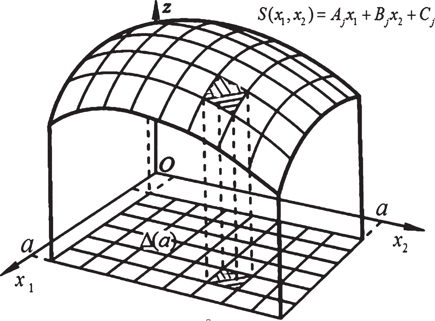
Let $ℝ^{n}$ represent n-dimensional. Euclidean space, $ℝ^{+}$ stands for positive axis [0, + ∞), $ℕ$ is the set of natural numbers, ρ is an Euclidean distance on $ℝ^{n}$ , [·] is an integer notation. We first give the concept of the PLF. For a given a > 0, if let $\begin{matrix} Δ (a) & = & {(x_{1}, x_{2}, \dots, x_{n}) \in ℝ^{n} | - a \leq x_{i} \leq a, \\ i = 1, 2, \dots, n; a > 0} . \end{matrix}$

Then Δ(a) is a generalized cube with the side length of 2a, it can is written as Δ(a) = [- a, a] ⁿ .

Definition 1. [13] Let a multivariable continuous function $S : ℝ^{n} \to ℝ$ . If the conditions ➀ to ➁ are satisfied as follows:

➀ There is a real number a > 0 such that S (x₁, x₂, ⋯ , x_n) is zero outside the Δ(a).

➁ If there is a group of n-dimensional polyhedrons Δ₁, Δ₂, ⋯ , Δ_{N
_S} with $⋃_{j = 1}^{N_{S}} Δ_{j} = Δ (a)$ (Δ_i ∩ Δ_j = ∅(i ≠ j), such that S is a linear function on Δ_j, that is, for any x = (x₁, x₂, ⋯ , x_n) ∈ Δ_j, it can be expressed as $S_{j} (x) = \sum_{i = 1}^{n} β_{ij} \cdot x_{i} + λ_{j}, j = 1, 2, \dots, N_{s} .$

Then S_j is called a piecewise linear function, shorthand for PLF, where β_ij, λ_j are constants.

$D (ℝ^{n})$ is marked as the set of all PLFs on $ℝ^{n}$ . For any $S \in D (ℝ^{n})$ , let V (S) be the set of all vertexes of the divided polyhedron Δ₁, Δ₂, ⋯ , Δ_{N
_S} of S, V (Δ_j) be the set of all vertexes of any Δ_j.

In fact, the PLF plays an important role as connector in the study of the approximation between Mamdani and T-S fuzzy systems, which can be attributed to the fact that fuzzy systems can be approximated to a PLF, and the PLF can be approximated to any continuous functions. In this way, we can realize the goal which a fuzzy system approximates to an unknown function.

Let $C (U) = {f : U \to ℝ | f$ is a continuous function on U}, where $U \subset ℝ^{n}$ is a compact set.

Definition 2. For every f ∈ C (U), let $| | f | |_{\infty} = \sup_{x \in U} | f (x) |$ , then || · ||_∞ is called a maximum norm or a infinite norm on C (U). For any f, g ∈ C (U), then $| | f - g | |_{\infty} = \sup_{x \in U} | f (x) - g (x) |$ .

Definition 3. Let $β \in ℝ$ , $b = (b_{1}, b_{2}, \dots, b_{n}) \in ℝ^{n}$ , $Ω (β) = {x = (x_{1}, x_{2}, \dots, x_{n}) \in ℝ^{n} | < x, b > = β}$ .

Then Ω (β) is called a β-hyperplane on $ℝ^{n}$ , where <· > is a inner product.

Obviously, β-hyperplane can be equivalently expressed the multivariate linear combination as $\begin{matrix} Ω (β) & = & {(x_{1}, x_{2}, \dots, x_{n}) \in ℝ^{n} | b_{1} x_{1} + b_{2} x_{2} \\ + \dots + b_{n} x_{n} = β, b_{i} \in ℝ, i = 1, 2, \dots, n} . \end{matrix}$

Definition 4. Let P be an n-order matrix, then the absolute value of the determinant |P| is called a matrix norm of P, write it as ||P|| = | (|P|) |. Distinctly, ||P|| can satisfy ||P||≥0.

3 Mesh construction of PLF

Next, according to the β-hyperplane and the polyhedron subdivision we would construct a PLF by the mesh construction on the compact set $U \subset ℝ^{n}$ . Let a continuous function f ∈ C (U).

Since U is a bounded set, there is a > 0 to enable U ⊂ [- a, a] ⁿ = Δ(a), and f is uniform continuous in the generalized cube Δ(a). In other words, for arbitrary ɛ > 0, there is δ > 0, for any x, y ∈ Δ(a) with ρ (x, y) < δ, then |f (x) - f (y) | < ɛ.

Step ➀ Mesh subdivision Δ(a). For every ɛ > 0, let $m_{0} = [a \sqrt{n} / δ] \in ℕ$ , when m > m₀. If 2m - 2 points are equidistant inserted in the straight line [- a, a], then 2m small closed intervals can be obtained. Similarly, the same equidistance subdivision is conducted for the rest n - 1 straight line segments. Hence, the mesh subdivision is formed on Δ(a), the generalized small cube $Δ_{i_{1} i_{2} \dots i_{n}} (\frac{a}{m})$ can be expressed as $Δ_{i_{1} i_{2} \dots, i_{n}} (\frac{a}{m}) = {(x_{1}, x_{2}, \dots, x_{n}) \in Δ (a) | \frac{i_{k} - 1}{m} a \leq x_{k} \leq \frac{i_{k}}{m} a,$ k = 1, 2, ⋯ , n ; i_k = 1 - m, 2 - m, ⋯ , 0, ⋯ , m - 1, m }.

For any $x = (x_{1}, x_{2}, \dots, x_{n}), y = (y_{1}, y_{2}, \dots, y_{n}) \in Δ_{i_{1} i_{2} \dots i_{n}} (\frac{a}{m})$ , if the Euclidean distance $\begin{matrix} ρ (x, y) \\ = \sqrt{(x_{1} - y_{1})^{2} + (x_{2} - y_{2})^{2} + \dots + (x_{n} - y_{n})^{2}} \\ \leq \sqrt{n (\frac{a}{m})^{2}} = \frac{a}{m} \sqrt{n} < δ . \end{matrix}$

We only need to select $m \geq [a \sqrt{n} / δ]$ , this is why we select m₀ in the front.

Step ➁ Categorizations for $Δ_{i_{1} i_{2} \dots i_{n}} (\frac{a}{m})$ . Let $Δ_{i_{1} i_{2} \dots i_{n}} (\frac{a}{m}) = Q_{j}$ , j = 1, 2, ⋯ , 2ⁿmⁿ, then 2ⁿmⁿ small cubes can be divided into three categories: The first category, the small cubes within U that are not adjacent to the boundary ∂U, which are noted as Σ^c (m); The second category, the small cubes inside or outside the U that are adjacent to the boundary, which are noted as ∑(m); The third category, all small cubes outside the ∑(m).

Obviously, the third category is not in our defined domain, thus, they will not be discussed in this research. See to Fig. 1.

Fig.1

The mesh subdivision of Δ(a) when n = 2.

Our research focused on the second category. Since every small cube in ∑(m) has a part that does not belong to U, we only considered the irregular polyhedron that belongs to U. It is inevitable that the total vertex number of the polyhedron may change slightly, as shown in Fig. 1.

Clearly, after the aggregation of the divided polyhedrons, the number is smaller than 2ⁿmⁿ. Let the total number be p, it can be written as $Q_{j} \in \sum (m) \cup \sum^{c} (m), j = 1, 2, \dots, p .$

Note 1. When n = 1, 2, 3, each generalized cube Q_j can be processed with the mesh subdivision using the traditional elementary geometric method. For example, when n = 1, Q_j degenerates into a closed interval [- a, a] (with 2 ends); when n = 2, Q_j can be divided into two isosceles right triangles according to leading diagonal line (with 3 vertexes); when n = 3, Q_j can be divided into 5 small tetrahedrons (with 4 vertexes), i.e., it can be divided into four identical triangular pyramids and one triangular pyramid with doubled volume. Yet unfortunately, when n ≥ 4, there is no coordinates system with the dimensionality larger than 4, it cannot be intuitively divided with the elementary geometric method. Thus, the hyperplane defined by inner product of vectors in Definition 3 can be applied to implement the abstract mesh subdivision, as shown in Literature [2].

We assume that each Q_j is abstractly processed with the mesh subdivision, and Q_j can generate a finite n-dime. polyhedrons {Δ_j1, Δ_j2, ⋯ , Δ_js}, j = 1, 2, ⋯ , p, which also satisfy $\cup_{i = 1}^{s} Δ_{ji} = Q_{j}, Δ_{ji} \cap Δ_{jk} = \emptyset (i \neq k)$ .

Identical mesh subdivision is implemented for each Q_j, the total number of small polyhedrons is the same. At this moment, it is not concerned that how many polyhedrons are divided from each Q_j, only noted as s, we only care about the total number of vertices after the subdivision of Δ_ji.

Step ➂ Identify hyperplane equation. Take a small polyhedron Δ_ji after the subdivision of Q_j, for arbitrary $x_{k}^{*} = (x_{1}^{k}, x_{2}^{k}, \dots, x_{n}^{k}) \in V (Δ_{ji}),$ k = 1, 2, ⋯ , n, n + 1. Assume n + 1 vertexes are not in the same hyperplane, thus ensuring the following determinant |D_n|≠0.

In addition, according to the designated rule, let n + 1 v vertex coordinates be $x_{1}^{*}, x_{2}^{*}, \dots, x_{n}^{*}, x_{n + 1}^{*}$ successively, and each $f (x_{k}^{*})$ can be determined.

Besides, the vertex coordinates of the hyperplane Δ_ji in (n + 1)-dimensional abstract space can be expressed the form of a vector as follows: $\begin{matrix} (x_{1}^{1}, x_{2}^{1}, \dots, x_{n}^{1}, f (x_{1}^{*})), (x_{1}^{2}, x_{2}^{2}, \dots, x_{n}^{2}, f (x_{2}^{*})), \\ \dots, (x_{1}^{n + 1}, x_{2}^{n + 1}, \dots, x_{n}^{n + 1}, f (x_{n}^{*})) . \end{matrix}$

In accordance with Definition 3, the hyperplane equation of n + 1 vertex coordinates in (n + 1)-dimensional abstract space can beset as $S_{ji} (x) = b_{j 1}^{i} x_{1} + b_{j 2}^{i} x_{2} + \dots + b_{jn}^{i} x_{n} + λ_{j}^{i},$ (1) where x = (x₁, x₂, ⋯ , x_n) ∈ Δ_ji; j = 1, 2, ⋯ , p; i = 1, 2, ⋯ , s.

In order to solve the analytic expression of the hyperplane S_ji (x), the key is to determine the coefficients $b_{j 1}^{i}, b_{j 2}^{i}, \dots, b_{jn}^{i}$ and $λ_{j}^{i}$ . Moreover, the hyperplane S_ji (x) and the curved surface f (x) have public vertexes in the polyhedron Δ_ji. Therefore, they are equal at each vertex $x_{k}^{*}$ , i.e., $S_{ji} (x_{k}^{*}) = f (x_{k}^{*}), k = 1, 2, \dots, n, n + 1 .$

Next, the vertexes $x_{1}^{*}, x_{2}^{*}, \dots, x_{n}^{*}, x_{n + 1}^{*}$ are successively substituted into Equation (1) on the hyperplane Δ_ji, then Equation (2) can be established as follows: ${\begin{matrix} f (x_{1}^{*}) = b_{ji}^{i} x_{1}^{1} + b_{j 2}^{i} x_{2}^{1} + \dots + b_{jn}^{i} x_{n}^{1} + λ_{j}^{i} \\ f (x_{2}^{*}) = b_{ji}^{i} x_{1}^{2} + b_{j 2}^{i} x_{2}^{2} + \dots + b_{jn}^{i} x_{n}^{2} + λ_{j}^{i} \\ \dots \dots \dots \dots \dots \dots \dots \\ f (x_{n}^{*}) = b_{ji}^{i} x_{1}^{n} + b_{j 2}^{i} x_{2}^{n} + \dots + b_{jn}^{i} x_{n}^{n} + λ_{j}^{i} \\ f (x_{n + 1}^{*}) = b_{ji}^{i} x_{1}^{n + 1} + \dots + b_{jn}^{i} x_{n}^{n + 1} + λ_{j}^{i} \end{matrix},$ (2) where $f (x_{k}^{*})$ is the corresponding value of the given data pairs $(x_{k}^{*}, f (x_{k}^{*}))$ , its value can be usually known.

Step ➃ Coefficient solution. For (n + 1)-dime. linear equation group (2), the unknown variables are $b_{j 1}^{i}, b_{j 2}^{i}, \dots, b_{jn}^{i}$ and $λ_{j}^{i}$ , where j = 1, 2, ⋯ , p; i = 1, 2, ⋯ , s. The coefficient matrixs are $\begin{matrix} D_{j 1}^{i} = (\begin{matrix} f (x_{1}^{*}) & x_{2}^{1} & \dots & x_{n}^{1} & 1 \\ f (x_{2}^{*}) & x_{2}^{2} & \dots & x_{n}^{2} & 1 \\ ⋮ & \dots & \dots & \dots & ⋮ \\ f (x_{n}^{*}) & x_{2}^{n} & \dots & x_{n}^{n} & 1 \\ f (x_{n + 1}^{*}) & x_{2}^{n + 1} & \dots & x_{n}^{n + 1} & 1 \end{matrix}), \\ D_{j 2}^{i} = (\begin{matrix} x_{1}^{1} & f (x_{1}^{*}) & \dots & x_{n}^{1} & 1 \\ x_{1}^{2} & f (x_{2}^{*}) & \dots & x_{n}^{2} & 1 \\ ⋮ & \dots & \dots & \dots & ⋮ \\ x_{1}^{n} & f (x_{n}^{*}) & \dots & x_{n}^{n} & 1 \\ x_{1}^{n + 1} & f (x_{n + 1}^{*}) & \dots & x_{n}^{n + 1} & 1 \end{matrix}), \dots, \\ D_{jn}^{i} = (\begin{matrix} x_{1}^{1} & x_{2}^{1} & \dots & f (x_{1}^{*}) & 1 \\ x_{1}^{2} & x_{2}^{2} & \dots & f (x_{2}^{*}) & 1 \\ ⋮ & \dots & \dots & \dots & ⋮ \\ x_{1}^{n} & x_{2}^{n} & \dots & f (x_{n}^{*}) & 1 \\ x_{1}^{n + 1} & x_{2}^{n + 1} & \dots & f (x_{n + 1}^{*}) & 1 \end{matrix}), \\ D_{j (n + 1)}^{i} = (\begin{matrix} x_{1}^{1} & x_{2}^{1} & \dots & x_{n}^{1} & f (x_{1}^{*}) \\ x_{1}^{2} & x_{2}^{2} & \dots & x_{n}^{2} & f (x_{2}^{*}) \\ ⋮ & \dots & \dots & \dots & ⋮ \\ x_{1}^{n} & x_{2}^{n} & \dots & x_{n}^{n} & f (x_{n}^{*}) \\ x_{1}^{n + 1} & x_{2}^{n + 1} & \dots & x_{n}^{n + 1} & f (x_{n + 1}^{*}) \end{matrix}), \\ D_{n} = (\begin{matrix} x_{1}^{1} & x_{2}^{1} & \dots & x_{n}^{1} & 1 \\ x_{1}^{2} & x_{2}^{2} & \dots & x_{n}^{2} & 1 \\ ⋮ & \dots & \dots & \dots & ⋮ \\ x_{1}^{n} & x_{2}^{n} & \dots & x_{n}^{n} & 1 \\ x_{1}^{n + 1} & x_{2}^{n + 1} & \dots & x_{n}^{n + 1} & 1 \end{matrix}) . \end{matrix}$

And the expression ${\begin{matrix} b_{j 1}^{i} = | D_{j 1}^{i} | / | D_{n} | \\ b_{j 2}^{i} = | D_{j 2}^{i} | / | D_{n} | \\ \dots \dots \dots \dots \dots \dots \\ b_{jn}^{i} = | D_{jn}^{i} | / | D_{n} | \\ λ_{j}^{i} = | D_{j (n + 1)}^{i} | / | D_{n} | \end{matrix}$ is a unique solution of Equation (2).

Step ➄ Mesh construction of PLF. the solution is substituted into Equation (1) to acquire the analytic equation of hyperplane equation S_ji (x) as $\begin{matrix} S_{ji} (x) \\ = \frac{| D_{j 1}^{i} |}{| D_{n} |} x_{1} + \frac{| D_{j 2}^{i} |}{| D_{n} |} x_{2} + \dots \\ + \frac{| D_{jn}^{i} |}{| D_{n} |} x_{n} + \frac{| D_{j (n + 1)}^{i} |}{| D_{n} |}, \end{matrix}$ for any x = (x₁, x₂, ⋯ , x_n) ∈ Δ_ji.

According to Definition 1, it is obvious that S_ji (x) is a continuous PLF on Δ_ji.

Similarly, if all the mesh polyhedron Δ_ji in $⋃_{j = 1}^{p} Q_{j}$ can be constructed by the above method, we can obtain a PLF on $ℝ^{n}$ as follows:

$\begin{matrix} S (x) \\ = {\begin{matrix} \frac{| D_{j 1}^{i} |}{| D_{n} |} x_{1} + \frac{| D_{j 2}^{i} |}{| D_{n} |} x_{2} + \dots + \frac{| D_{jn}^{i} |}{| D_{n} |} x_{n} + \frac{| D_{j (n + 1)}^{i} |}{| D_{n} |} \\ x = (x_{1}, x_{2}, \dots, x_{n}) \in Δ_{ji} \\ 0, x = (x_{1}, x_{2}, \dots, x_{n}) \in Δ^{c} (a) \\ j = 1, 2, \dots, p; i = 1, 2, \dots, s \end{matrix}, \end{matrix}$ (3)

In accordance with the Step ➂, S and f in all vertexes $x_{k}^{*} = (x_{1}^{k}, x_{2}^{k}, \dots, x_{n}^{k})$ of the divided polyhedron Δ_ji are identical. That is, $S (x_{k}^{*}) = f (x_{k}^{*}), k = 1, 2, \dots, n, n + 1 .$

In addition, it can be found that after mesh subdivision for Δ(a), the coordinates of any moving point in each small polyhedron Δ_ji can be expressed by vertex coordinates of Δ_ji. With n = 2 as an example, for arbitrary (x₁, x₂) ∈ Δ(a), there exists an isosceles right triangle Δ_ji to enable (x₁, x₂) ∈ Δ_ji. When the subdivide number m is determined, its vertex coordinates can also be identified, and the length of the right-angle side is $\frac{a}{m}$ . Let the three vertex coordinates of Δ_ji are $(x_{1}^{1}, x_{2}^{1}), (x_{1}^{2}, x_{2}^{2})$ and $(x_{1}^{3}, x_{2}^{3})$ .

Obviously, the component coordinates can meet $x_{1}^{1} = x_{1}^{3}, x_{2}^{1} = x_{2}^{2}$ , as shown in Fig. 3.

Fig.2

The local graph of PLF when n = 2.

Fig.3

Decomposition graph in x₁ox₂ when n = 2.

Let a moving point (x₁, x₂) ∈ Δ_ji, the parameters λ₁, λ₂, θ₁, θ₂ ∈(0, 1), and satisfy λ₁ + λ₂ = 1 and θ₁ + θ₂ = 1. According to Fig. 3, the relations of the component of the vertex coordinates and the moving point are as follows: $\begin{matrix} {\begin{matrix} x_{1}^{1} = x_{1} - \frac{a θ_{1}}{m} \\ x_{2}^{1} = x_{2} - \frac{a λ_{1}}{m} \end{matrix}, \\ {\begin{matrix} x_{1}^{2} = x_{1} + \frac{a θ_{2}}{m} \\ x_{2}^{2} = x_{2} - \frac{a λ_{1}}{m} \end{matrix}, \\ {\begin{matrix} x_{1}^{3} = x_{1} - \frac{a θ_{1}}{m} \\ x_{2}^{3} = x_{2} + \frac{a λ_{2}}{m} \end{matrix} . \end{matrix}$

Obviously, the formulas of the component coordinates along x₁-axis and x₂-axis are as follows: $\begin{matrix} \frac{a i_{j}}{m} = x_{1}^{j} = x_{1} \pm \frac{a θ_{j}}{m}, \\ \frac{a i_{j}}{m} = x_{2}^{j} = x_{2} \pm \frac{a λ_{j}}{m}, \end{matrix}$ where j = 1, 2, 3; i₁, i₂, i₃ ∈ {1, 2, 3}, and satisfy $x_{1}^{1} = x_{1}^{3}$ , $x_{2}^{1} = x_{2}^{2}$ , θ₃ = θ₁ and λ₃ = λ₁.

For any moving point x = (x₁, x₂) ∈ Δ(a), the component x_j and the vertex component $\frac{a i_{j}}{m}$ of the corresponding polyhedron Δ_ji are satisfied as follows:

$\begin{matrix} \frac{a i_{j}}{m} & = & x_{j} \pm \frac{a θ_{j}}{m} \Rightarrow | x_{j} - \frac{a i_{j}}{m} | \\ = & \frac{a θ_{j}}{m} \leq \frac{a}{m}, j = 1, 2 . \end{matrix}$ (4)

Of course, if for n-dimension input x = (x₁, x₂, ⋯ , x_n) ∈ Δ(a), the formula (4) is also established.

4 Approximation of PLF

Usually, the analytical expression of a specific PLF is very practical, it is natural to think over whether the PLF has approximation performance for the given continuous function? What about the efficiency of its approximation? In this section, the previous question will be answered and proved, and lay a foundation for further to study that Mamdani fuzzy system approximate to a continuous function.

Theorem 1. Let a given compact set $U \subset ℝ^{n}$ , f ∈ C (U), and {Δ_j1, Δ_j2, ⋯ , Δ_{j
_s}} is the mesh subdivision polyhedron of j-th generalized cube Q_j(j = 1, 2, ⋯ , p), if denoted $x_{k}^{*} = (x_{1}^{k}, x_{2}^{k}, \dots, x_{n}^{k})$ (k = 1, 2, ⋯ , n + 1) as n + 1 vertex coordinates of the n-dimensional polyhedron Δ_ji. Then, for arbitrary ɛ > 0, there is a > 0 and a PLF $S \in D (ℝ^{n})$ to enable ∥f - S ∥ _∞ < ɛ, i.e., the mesh PLF S can approximate to the continuous function f for arbitrary accuracy with respect to the maximum norm || · ||_∞.

Proof. Because f is continuous on the compact set U, a PLF can be constructed through the Steps ➀-➄, we only need to verify that the S can approximate to f. The involved symbols in the following processes of verification are consistent with the above requirements.

In fact, for arbitrary x = (x₁, x₂, ⋯ , x_n) ∈ Δ(a), there is only j ∈ {1, 2, ⋯ , p} and i ∈ {1, 2, ⋯ , s} lead to x ∈ Δ_ji. Specially, the determinant $| D_{j (n + 1)}^{i} |$ on the constant term of PLF can be obtained from Step ➃. According to some properties of a determinant, we have $\begin{matrix} | D_{j (n + 1)}^{i} | \\ = | \begin{matrix} x_{1}^{1} - x_{1}^{2} & x_{2}^{1} - x_{2}^{2} & \dots & x_{n}^{1} - x_{n}^{2} & f (x_{1}^{*}) - f (x_{2}^{*}) \\ x_{1}^{2} - x_{1}^{3} & x_{2}^{2} - x_{2}^{3} & \dots & x_{n}^{2} - x_{n}^{3} & f (x_{2}^{*}) - f (x_{3}^{*}) \\ ⋮ & \dots & \dots & \dots & ⋮ \\ x_{1}^{n} - x_{1}^{n + 1} & x_{2}^{n} - x_{2}^{n + 1} & \dots & x_{n}^{n} - x_{n}^{n + 1} & f (x_{n}^{*}) - f (x_{n + 1}^{*}) \\ x_{1}^{n + 1} & x_{2}^{n + 1} & \dots & x_{n}^{n + 1} & f (x_{n + 1}^{*}) \end{matrix} | \\ = {(- 1)}^{n} | D_{n 1} | (f (x_{1}^{*}) - f (x_{2}^{*})) {+ (- 1)}^{n - 1} | D_{n 2} | (f (x_{2}^{*}) \\ - f (x_{3}^{*})) + \dots - | D_{nn} | (f (x_{n}^{*}) - f (x_{n + 1}^{*})) \\ + | D_{n} | f (x_{n + 1}^{*}) . \end{matrix}$

The corresponding coefficient determinants as $\begin{matrix} | D_{n 1} | & = & | \begin{matrix} x_{1}^{2} - x_{1}^{3} & x_{2}^{2} - x_{2}^{3} & \dots & x_{n}^{2} - x_{n}^{3} \\ ⋮ & \dots & \dots & ⋮ \\ x_{1}^{n} - x_{1}^{n + 1} & x_{2}^{n} - x_{2}^{n + 1} & \dots & x_{n}^{n} - x_{n}^{n + 1} \\ x_{1}^{n + 1} & x_{2}^{n + 1} & \dots & x_{n}^{n + 1} \end{matrix} |, \\ | D_{n 2} | & = & | \begin{matrix} x_{1}^{1} - x_{1}^{2} & x_{2}^{1} - x_{2}^{2} & \dots & x_{n}^{1} - x_{n}^{2} \\ ⋮ & \dots & \dots & ⋮ \\ x_{1}^{n} - x_{1}^{n + 1} & x_{2}^{n} - x_{2}^{n + 1} & \dots & x_{n}^{n} - x_{n}^{n + 1} \\ x_{1}^{n + 1} & x_{2}^{n + 1} & \dots & x_{n}^{n + 1} \end{matrix} |, \\ \dots \dots \dots \dots \dots \dots \\ | D_{nn} | & = & | \begin{matrix} x_{1}^{1} - x_{1}^{2} & x_{2}^{1} - x_{2}^{2} & \dots & x_{n}^{1} - x_{n}^{2} \\ x_{1}^{2} - x_{1}^{3} & x_{2}^{2} - x_{2}^{3} & \dots & x_{n}^{2} - x_{n}^{3} \\ ⋮ & \dots & \dots & ⋮ \\ x_{1}^{n + 1} & x_{2}^{n + 1} & \dots & x_{n}^{n + 1} \end{matrix} |, \\ | D_{n} | & = & | \begin{matrix} x_{1}^{1} - x_{1}^{2} & x_{2}^{1} - x_{2}^{2} & \dots & x_{n}^{1} - x_{n}^{2} \\ x_{1}^{2} - x_{1}^{3} & x_{2}^{2} - x_{2}^{3} & \dots & x_{n}^{2} - x_{n}^{3} \\ ⋮ & \dots & \dots & ⋮ \\ x_{1}^{n} - x_{1}^{n + 1} & x_{2}^{n} - x_{2}^{n + 1} & \dots & x_{n}^{n} - x_{n}^{n + 1} \end{matrix} | . \end{matrix}$

Therefore, the constant term of Equation (3) can be expressed as follows:

$\begin{matrix} \frac{| D_{j (n + 1)}^{i} |}{| D_{n} |} = (- 1)^{n} \frac{| D_{n 1} |}{| D_{n} |} (f (x_{1}^{*}) - f (x_{2}^{*})) \\ + (- 1)^{n - 1} \frac{| D_{n 2} |}{| D_{n} |} (f (x_{2}^{*}) - f (x_{3}^{*})) + \dots \\ - \frac{| D_{nn} |}{| D_{n} |} (f (x_{n}^{*}) - f (x_{n + 1}^{*})) + f (x_{n + 1}^{*}) . \end{matrix}$ (5)

Besides, for the matrix determinants $| D_{j 1}^{i} |,$ $| D_{j 2}^{i} |, \dots, | D_{jn}^{i} |$ , they can be unfolded as

$\begin{matrix} | D_{j 1}^{i} | x_{1} + | D_{j 2}^{i} | x_{2} + \dots + | D_{jn}^{i} | x_{n} \\ = | \begin{matrix} f (x_{1}^{*}) - f (x_{2}^{*}) & x_{2}^{1} - x_{2}^{2} & \dots & x_{n}^{1} - x_{n}^{2} \\ f (x_{2}^{*}) - f (x_{3}^{*}) & x_{2}^{2} - x_{2}^{3} & \dots & x_{n}^{2} - x_{n}^{3} \\ ⋮ & \dots & \dots & ⋮ \\ f (x_{n}^{*}) - f (x_{n + 1}^{*}) & x_{2}^{n} - x_{2}^{n + 1} & \dots & x_{n}^{n} - x_{n}^{n + 1} \end{matrix} | x_{1} \\ + | \begin{matrix} x_{1}^{1} - x_{1}^{2} & f (x_{1}^{*}) - f (x_{2}^{*}) & \dots & x_{n}^{1} - x_{n}^{2} \\ x_{1}^{2} - x_{1}^{3} & f (x_{2}^{*}) - f (x_{3}^{*}) & \dots & x_{n}^{2} - x_{n}^{3} \\ ⋮ & \dots & \dots & ⋮ \\ x_{1}^{n} - x_{1}^{n + 1} & f (x_{n}^{*}) - f (x_{n + 1}^{*}) & \dots & x_{n}^{n} - x_{n}^{n + 1} \end{matrix} | x_{2} \\ + \cdot \cdot \cdot \\ + | \begin{matrix} x_{1}^{1} - x_{1}^{2} & x_{2}^{1} - x_{2}^{2} & \dots & f (x_{1}^{*}) - f (x_{2}^{*}) \\ x_{1}^{2} - x_{1}^{3} & x_{2}^{2} - x_{2}^{3} & \dots & f (x_{2}^{*}) - f (x_{3}^{*}) \\ ⋮ & \dots & \dots & ⋮ \\ x_{1}^{n} - x_{1}^{n + 1} & x_{2}^{n} - x_{2}^{n + 1} & \dots & f (x_{n}^{*}) - f (x_{n + 1}^{*}) \end{matrix} | x_{n} \\ = (f (x_{1}^{*}) - f (x_{2}^{*})) \\ (| B_{1}^{1} | x_{1} - | B_{2}^{1} | x_{2} + \dots + (- 1)^{n - 1} | B_{n}^{1} | x_{n}) \\ + (f (x_{2}^{*}) - f (x_{3}^{*})) (- | B_{1}^{2} | x_{1} + | B_{2}^{2} | x_{2} \\ + \dots + (- 1)^{n} | B_{n}^{2} | B_{n}^{2} x_{n}) + \dots \\ + (f (x_{n}^{*}) - f (x_{n + 1}^{*})) ((- 1)^{n - 1} | B_{1}^{n} | x_{1} \\ + (- 1)^{n} | B_{2}^{n} | x_{2} + \dots + | B_{n}^{n} | x_{n}), \end{matrix}$ (6)

where $| B_{l}^{1} | (l = 1, 2, \dots, n)$ is the corresponding (n - 1)-order algebraic complementary determinant in the first column unfolding of the first determinant $| B_{l}^{2} |$ is the corresponding (n - 1)-order algebraic complementary determinant in the second column unfolding of the second determinant. The rest can be done in the same manner. For example, $\begin{matrix} | B_{2}^{1} | & = & | \begin{matrix} x_{1}^{2} - x_{1}^{3} & \dots & x_{n}^{2} - x_{n}^{3} \\ ⋮ & \dots & ⋮ \\ x_{1}^{n} - x_{1}^{n + 1} & \dots & x_{1}^{n} - x_{1}^{n + 1} \end{matrix} | or \\ | B_{2}^{2} | & = & | \begin{matrix} x_{1}^{1} - x_{1}^{2} & \dots & x_{n}^{1} - x_{n}^{2} \\ ⋮ & \dots & ⋮ \\ x_{1}^{n} - x_{1}^{n + 1} & \dots & x_{n}^{n} - x_{n}^{n + 1} \end{matrix} | . \end{matrix}$

When Equations (5) and (6) were substituted in Equation (3), for any x = (x₁, x₂, ⋯ , x_n) ∈ Δ(a), we can obtain

$\begin{matrix} | | D_{n} | | \cdot | f (x) - S (x) | \leq | | B_{1}^{1} | x_{1} - | B_{2}^{1} | x_{2} + \dots \\ + (- 1)^{n - 1} | B_{n}^{1} | x_{n} + (- 1)^{n} | D_{n 1} | | \cdot | f (x_{1}^{*}) - f (x_{2}^{*}) | \\ + | - | B_{1}^{2} | x_{1} + | B_{2}^{2} | x_{2} + \dots + (- 1)^{n} | B_{n}^{2} | B_{n}^{2} x_{n} + \\ (- 1)^{n - 1} | D_{n 2} | | \cdot | f (x_{2}^{*}) - f (x_{3}^{*}) | + \dots \\ + | (- 1)^{n - 1} | B_{1}^{n} | x_{1} + (- 1)^{n} | B_{2}^{n} | x_{2} + \dots + | B_{n}^{n} | x_{n} - | D_{nn} | | \\ \times | f (x_{n}^{*}) - f (x_{n + 1}^{*}) | + | f (x_{n + 1}^{*}) - f (x) | . \end{matrix}$ (7)

In accordance with the last line unfolding each determinant |D_n1|, |D_n2| , ⋯ , |D_nn|, we can get ${\begin{matrix} | D_{n 1} | = (- 1)^{n + 1} | B_{1}^{1} | x_{1}^{n + 1} + (- 1)^{n} | B_{2}^{1} | x_{2}^{n + 1} \\ + \dots + | B_{n}^{1} | x_{n}^{n + 1} \\ | D_{n 2} | = (- 1)^{n + 1} | B_{1}^{2} | x_{1}^{n + 1} + (- 1)^{n} | B_{2}^{2} | x_{2}^{n + 1} \\ + \dots + | B_{n}^{2} | x_{n}^{n + 1} \\ \dots \dots \dots \dots \dots \dots \dots \dots \dots \dots \\ | D_{nn} | = (- 1)^{n + 1} | B_{1}^{n} | x_{1}^{n + 1} + (- 1)^{n} | B_{2}^{n} | x_{2}^{n + 1} \\ + \dots + | B_{n}^{n} | x_{n}^{n + 1} \end{matrix},$ (8)

For every x = (x₁, x₂, ⋯ , x_n) ∈ Δ_ji, then the coordinate components $x_{i}^{k}$ of each vertex in the Δ_ji are satisfied the inequation $\begin{matrix} | x_{i} - x_{i}^{k} | \\ \leq \frac{a}{m}, i = 1, 2, \dots, n; k = 1, 2, \dots, n + 1, \end{matrix}$ where $\frac{a}{m}$ is the side length of Δ_ji.

In addition, the distances $∥ x_{k}^{*} - x_{k + 1}^{*} ∥$ and $∥ x_{n + 1}^{*} - x ∥$ in the polyhedron Δ_ji can be denoted as $\begin{matrix} ∥ x_{k}^{*} - x_{k + 1}^{*} ∥ \\ = \sqrt{(x_{1}^{k} - x_{1}^{k + 1})^{2} + (x_{2}^{k} - x_{2}^{k + 1})^{2} + \dots + (x_{n}^{k} - x_{n}^{k + 1})^{2}} \\ \leq \frac{a}{m} \sqrt{n} \to 0 (m \to \infty) . \\ ∥ x_{n + 1}^{*} - x ∥ \\ = \sqrt{(x_{1}^{n + 1} - x_{1})^{2} + (x_{2}^{n + 1} - x_{2})^{2} + \dots + (x_{n}^{n + 1} - x_{n})^{2}} \\ \leq \frac{a}{m} \sqrt{n} \to 0 (m \to \infty) . \end{matrix}$

Because the f (x) is uniformly continuous on Δ_ji, then for every ɛ > 0, we have the following conclusions $| f (x_{k}^{*}) - f (x_{k + 1}^{*}) | < ɛ, | f (x_{n + 1}^{*}) - f (x) | < ɛ .$ (9)

On the other hand, for |D_n1| we can obtain that $\begin{matrix} | | B_{1}^{1} | x_{1} - | B_{2}^{1} | x_{2} + \dots + (- 1)^{n - 1} | B_{n}^{1} | x_{n} + (- 1)^{n} | D_{n 1} | | \\ \leq | x_{1} - x_{1}^{n + 1} | \cdot | | B_{1}^{1} | | + | x_{2} - x_{2}^{n + 1} | \cdot | | B_{2}^{1} | | + \dots \\ + | x_{n} - x_{n}^{n + 1} | \cdot | | B_{n}^{1} | | \leq \frac{a}{m} (| | B_{1}^{1} | | + | | B_{2}^{1} | | + \dots + | | B_{n}^{1} | |) . \end{matrix}$

Similarly, for |D_n2| , ⋯ , |D_nn| we alsohave $\begin{matrix} | - | B_{1}^{2} | x_{1} + | B_{2}^{2} | x_{2} + \dots + (- 1)^{n} | B_{n}^{2} | B_{n}^{2} x_{n} \\ + (- 1)^{n - 1} | D_{n 2} | | \\ \leq \frac{a}{m} (| | B_{1}^{2} | | + | | B_{2}^{2} | | + \dots + | | B_{n}^{2} | |), \\ \dots \dots \dots \dots \dots \dots \dots \dots \\ | (- 1)^{n - 1} | B_{1}^{n} | x_{1} + (- 1)^{n} | B_{2}^{n} | x_{2} + \dots \\ + | B_{n}^{n} | x_{n} - | D_{mn} | | \\ \leq \frac{a}{m} (| | B_{1}^{n} | | + | | B_{2}^{n} | | + \dots + | | B_{n}^{n} | |), \end{matrix}$ where $| | B_{l}^{1} | |, | | B_{l}^{2} | |, \dots, | | B_{l}^{n} | |$ are the corresponding (n - 1)-order matrix norms, l = 1, 2, ⋯ , n.

Now, if the formula (9) is introduced into the formula (7), then we can obtain that $\begin{matrix} | f (x) - S (x) | \\ \leq \frac{a ɛ}{m | | D_{n} | |} ((| | B_{1}^{1} | | + | | B_{2}^{1} | | + \dots + | | B_{n}^{1} | |) \\ + (| | B_{1}^{2} | | + | | B_{2}^{2} | | + \dots + | | B_{n}^{2} | |) + \dots \\ + (| | B_{1}^{n} | | + | | B_{2}^{n} | | + \dots + | | B_{n}^{n} | |)) + ɛ \\ = (\frac{a}{m | | D_{n} | |} \sum_{l = 1}^{n} \sum_{k = 1}^{n} | | B_{k}^{l} | | + 1) ɛ . \end{matrix}$

According to the mesh subdivision and the properties of the determinants, it is not difficult to prove $\sum_{l - 1}^{n} \sum_{k = 1}^{n} | | B_{k}^{l} | | = k_{0} (\frac{a}{m})^{n - 1}$ , where k₀ is a constant, $\frac{a}{m}$ stands for the side length of small square $Δ_{i_{1}, i_{2}, \dots, i_{n}} (\frac{a}{m})$ .

On the other hand, because the matrix norm ||D_n|| is a generalized volume of the generalized cube Q_j, and its volume $| | D_{n} | | = (\frac{a}{m})^{n}$ . Hence, we can obtained that $0 < \frac{a}{m | | D_{n} | |} \sum_{l = 1}^{n} \sum_{k = 1}^{n} | | B_{k}^{l} | | = \frac{{ak}_{0} (\frac{a}{m})^{n - 1}}{m (\frac{a}{m})^{n}} = k_{0} .$

Hence, we immediately get that ${∥ f - S ∥}_{\infty} = sup_{x \in U} | f (x) - S (x) | < k_{0} ɛ .$

Consequently, the PLF S can approximate to f for arbitrary accuracy with respect to || · ||_∞.

5 Approximation

In fact, the construction of an effective fuzzy system based on existing information is much more difficult than verifying its existence. For arbitrary $x = (x_{1}, x_{2}, \dots, x_{n}) \in U \subset ℝ^{n}$ , we first give the following model (10) of Mamdani fuzzy system as

$\begin{matrix} F_{m} (x_{1}, x_{2}, \dots, x_{n}) = \\ \frac{\sum_{i_{1} = 1}^{N_{1}} \sum_{i_{2} = 1}^{N_{2}} \dots \sum_{i_{n} = 1}^{N_{n}} (\prod_{j = 1}^{n} {\tilde{A}}_{i_{j}}^{j} (x_{j})) \cdot {\bar{y}}_{i_{1} i_{2} \dots i_{n}}}{\sum_{i_{1} = 1}^{N_{1}} \sum_{i_{2} = 1}^{N_{2}} \dots \sum_{i_{n} = 1}^{N_{n}} (\prod_{j = 1}^{n} {\tilde{A}}_{i_{j}}^{j} (x_{j}))}, \end{matrix}$ (10) where ${\bar{y}}_{i_{1} i_{2} \dots i_{n}}$ is a center of the output fuzzy set byl-th fuzzy rule in Equation (10), other symbols can refer to Refs. [9, 10]. However, it is crucial to adequately select the center point ${\bar{y}}_{i_{1} i_{2} \dots i_{n}}$ .

Theorem 2. Let S a PLF of the form such as (6), the Mamdani fuzzy system is given by Equation (3), a > 0, and Δ(a) = [- a, a] ⁿ, {Δ_j1, Δ_j2, ⋯ , Δ_js} is the mesh subdivision polyhedron of the generalized small cube Q_j (j = 1, 2, ⋯ , p). Then for arbitrary ɛ > 0, there is a F_m such that ∥F_m - S ∥ _∞ < ɛ.

Proof. According to the assumption, for arbitrary x = (x₁, x₂, ⋯ , x_n) ∈ Δ(a), there is a m-mesh subdivision and the unique i, j to enable x ∈ Δ_j i, where Δ_ji is a small polyhedron, i and j are given, and every vertex $x_{k}^{*} = (x_{1}^{k}, x_{2}^{k}, \dots, x_{n}^{k})$ of Δ_ji s substituted into Equation (3), we have

$\begin{matrix} S (x_{k}^{*}) = \frac{| D_{j 1}^{i} |}{| D_{n} |} x_{1}^{k} + \dots + \frac{| D_{jn}^{i} |}{| D_{n} |} x_{n}^{k} + \frac{| D_{j (n + 1)}^{i} |}{| D_{n} |}, \\ k = 1, 2, \dots, n, n + 1 . \end{matrix}$ (11)

Clearly, based on the formula (4) and Definition 4 (matrix norm) we can obtain that $\begin{matrix} | S (x) - S (x_{k}^{*}) | \\ = \frac{1}{| | D_{n} | |} | | D_{j 1}^{i} | (x_{1} - x_{1}^{k}) + \dots + | D_{jn}^{i} | (x_{n} - x_{n}^{k}) | \\ \leq \frac{1}{| | D_{n} | |} \frac{a}{m} (| | D_{j 1}^{i} | | + | | D_{j 2}^{i} | | + \dots + | | D_{jn}^{i} | |) . \end{matrix}$

According to the definition of the coefficient matrix $D_{j 1}^{1}$ and determinant’s property, we have

$\begin{matrix} | D_{j 1}^{1} | & = & | \begin{matrix} f (x_{1}^{*}) - f (x_{2}^{*}) & x_{2}^{1} - x_{2}^{2} & \dots & x_{n}^{1} - x_{n}^{2} \\ f (x_{2}^{*}) - f (x_{3}^{*}) & x_{2}^{2} - x_{2}^{3} & \dots & x_{n}^{2} - x_{n}^{3} \\ ⋮ & \dots & \dots & ⋮ \\ f (x_{n}^{*}) - f (x_{n + 1}^{*}) & x_{2}^{n} - x_{2}^{n + 1} & \dots & x_{n}^{n} - x_{n}^{n + 1} \end{matrix} | \\ = & (f (x_{1}^{*}) - f (x_{2}^{*})) | B_{1}^{1} | - (f (x_{2}^{*}) - f (x_{3}^{*})) | B_{1}^{2} | \\ + \dots + (- 1)^{n - 1} (f (x_{n}^{*}) - f (x_{n + 1}^{*})) | B_{1}^{n} | . \end{matrix}$

In accordance with the formula (8) and matrix norm’s definition, for arbitrary ɛ > 0, there is $| | D_{j 1}^{1} | | < (| | B_{1}^{1} | | + | | B_{1}^{2} | | + \dots + | | B_{1}^{n} | |) ɛ .$

In the same way, there are also $\begin{matrix} | | D_{j 2}^{2} | | < (| | B_{2}^{1} | | + | | B_{2}^{2} | | + \dots + | | B_{2}^{n} | |) ɛ, \\ \dots \dots \dots \dots \dots \dots \dots \\ | | D_{jn}^{n} | | < (| | B_{n}^{1} | | + | | B_{n}^{2} | | + \dots + | | B_{n}^{n} | |) ɛ . \end{matrix}$

If write $\frac{a}{m | | D_{n} | |} \sum_{l = 1}^{n} \sum_{k = 1}^{n} | | B_{k}^{l} | | = k_{0}$ , we can get

$\begin{matrix} | S (x) - S (x_{k}^{*}) | \\ < (\frac{1}{| | D_{n} | |} \frac{a}{m} \sum_{l = 1}^{n} \sum_{k = 1}^{n} | | B_{k}^{l} | |) ɛ = k_{0} ɛ . \end{matrix}$ (12)

Let $x_{i_{1} i_{2} \dots i_{n}}^{*} = (x_{1}^{i_{1}}, x_{2}^{i_{2}}, \dots, x_{n}^{i_{n}})$ represent as the vertex coordinates of every small polyhedron Δ_ji after subdivision (the above $x_{k}^{*}$ is only one of them). If we select the center ${\bar{y}}_{i_{1} i_{2} \dots i_{n}}$ of the output fuzzy sets as ${\bar{y}}_{i_{1} i_{2} \dots i_{n}} = S (x_{i_{1} i_{2} \dots i_{n}}^{*}) = S (x_{1}^{i_{1}}, x_{2}^{i_{2}}, \dots, x_{n}^{i_{n}}) .$

For all vertexes $x_{i_{1} i_{2} \dots i_{n}}^{*}$ the formula (12) still is established. Thus, for any x = (x₁, x₂, ⋯ , x_n) ∈ Δ(a), according to the Mamdani fuzzy system model (10), we can obtain that $\begin{matrix} | F_{m} (x_{1}, x_{2}, \dots, x_{n}) - S (x_{1}, x_{2}, \dots, x_{n}) | \\ \leq \frac{\sum_{i_{1} = 1}^{N_{1}} \sum_{i_{2} = 1}^{N_{2}} \dots \sum_{i_{n} = 1}^{N_{n}} (\prod_{j = 1}^{n} {\tilde{A}}_{i_{j}}^{j} (x_{j})) \cdot | S (x_{i_{1} i_{2} \dots i_{n}}^{*}) - S (x) |}{\sum_{i_{1} = 1}^{N_{1}} \sum_{i_{2} = 1}^{N_{2}} \dots \sum_{i_{n} = 1}^{N_{n}} (\prod_{j = 1}^{n} {\tilde{A}}_{i_{j}}^{j} (x_{j}))} \\ < (\frac{1}{| | D_{n} | |} \frac{a}{m} \sum_{l = 1}^{n} \sum_{k = 1}^{n} | | B_{k}^{l} | |) ɛ \cdot 1 = k_{0} ɛ . \end{matrix}$

Based on the definition of the maximum norm|| · ||_∞, for arbitrary ɛ > 0, it is easy to prove that ${∥ F - S ∥}_{\infty} = sup_{x \in U} | F (x) - S (x) | \leq k_{0} ɛ .$

Therefore, the Mamdani fuzzy system F_m can approximate to S for arbitrary accuracy.

Corollary 1. Let f ∈ C (U), $U \subset ℝ^{n}$ is a compact set, S is a PLF of the form such as (6), the Mamdani fuzzy system is given by Equation (10). Then for arbitrary ɛ > 0, there is a F_m such that ∥ F_m - f ∥ _∞ < ɛ.

Proof. By Theorem 1, there are a m-mesh subdivision and a PLF S of the form such as (3), and S can approximate f with || · ||_∞, i.e., for arbitrary ɛ > 0, exists a PLF S such that ${∥ S - f ∥}_{\infty} < ɛ / 2 .$

By Theorem 2, for the above PLF S, there is a Mamdani fuzzy system F_m, and it can also approximate to S with respect to || · ||_∞, i.e., ${∥ F_{m} - S ∥}_{\infty} < ɛ / 2 .$

Hence, we immediately obtain that $\begin{matrix} {∥ F_{m} - f ∥}_{\infty} \leq {∥ F_{m} - S ∥}_{\infty} \\ + {∥ S - f ∥}_{\infty} < \frac{ɛ}{2} + \frac{ɛ}{2} = ɛ . \end{matrix}$

Therefore, the Mamdani fuzzy system F_m can approximate to f for arbitrary accuracy.

5 Simulation example

To facilitate the simulation, a two-dimensional continuous function was given. Next, on the basis of Steps ➀–➄, a specific PLF was constructed, and then, a PLF can approximate to the continuous function through a simulation example. Besides, the Mamdani fuzzy system have also a approximation performance to a PLF.

Example 1. Let a = 1, n = 2, for a given two-dimensional continuous function as $f (x, y) = 2 e^{- \frac{1}{4} (x^{2} + y^{2})}, (x, y) \in [- 1, 1] \times [- 1, 1] .$

Firstly, we may determine the subdivide number m₀: As f (x, y) is continuous on the compact set [-1, 1] × [-1, 1]. For simplicity, the construction of the two-dimensional PLF was confined in the first quadrant [0, 1] × [0, 1]. It is obvious that f is differentiable, and satisfy $\begin{matrix} | \frac{\partial f}{\partial x} | = | x e^{- \frac{1}{4} (x^{2} + y^{2})} | \leq 1, \\ | \frac{\partial f}{\partial y} | = | y e^{- \frac{1}{4} (x^{2} + y^{2})} | \leq 1 . \end{matrix}$

For any (x₁, y₁) , (x₂, y₂) ∈ [0, 1] × [0, 1], when |x₁ - x₂| < δ, |y₁ - y₂| < δ, according to the differential mean value theorem of multivariate function we can obtained that $\begin{matrix} | f (x_{1}, y_{1}) - f (x_{2}, y_{2}) | \\ \leq | \frac{\partial f}{\partial x} | x = ξ_{1} | \cdot | x_{1} - x_{2} | + | \frac{\partial f}{\partial y} | y = ξ_{2} | \cdot | y_{1} - y_{2} | \\ \leq | x_{1} - x_{2} | + | y_{1} - y_{2} | \leq 2 δ . \end{matrix}$

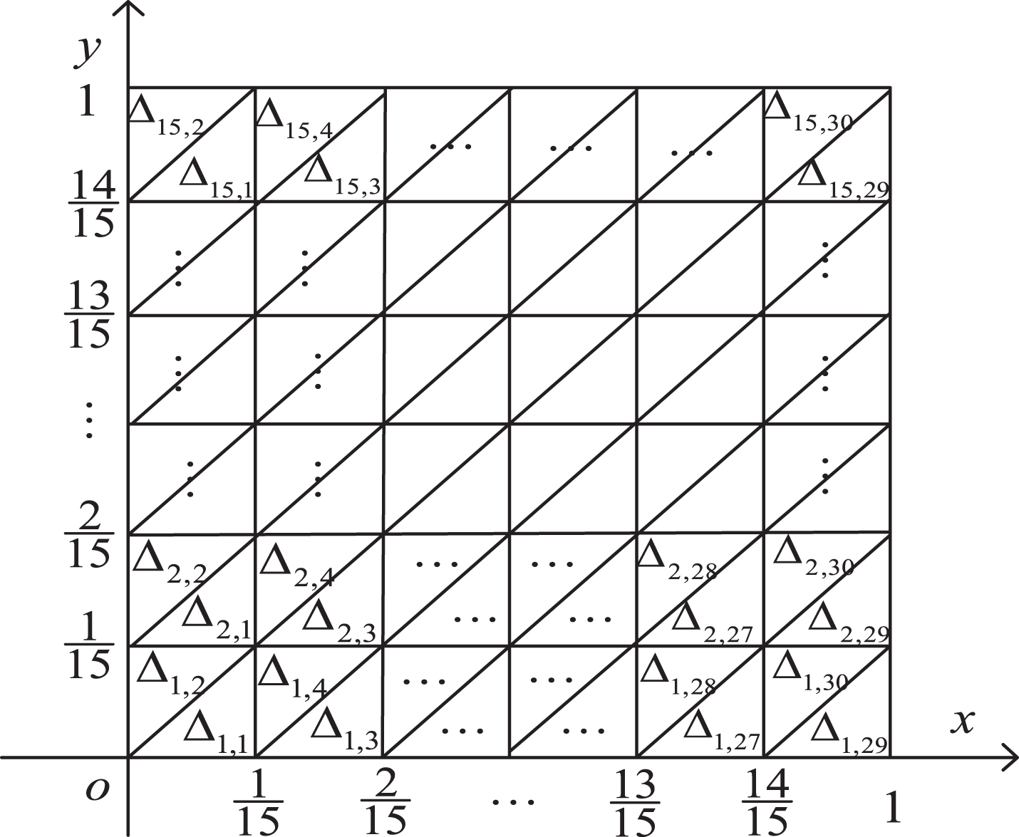
Take the accuracy ɛ = 0.2 > 0, $δ = \frac{ɛ}{2} = \frac{1}{10}$ . By the mesh subdivision Step ➀, the smallest subdivision number m₀ can be obtained, i.e., $m_{0} = \frac{1 \times \sqrt{2}}{δ} = 10 \sqrt{2} \approx 14.14 .$

Without loss of generality, we may chose m = 15. Now we only carried out the mesh subdivision in the square [0, 1] × [0, 1], a total of 15 × 15 = 225 small squares, write them as Δ_1,1, Δ_1,2, Δ_1,3, ⋯ , Δ_2,1, ⋯ , Δ_15,1, ⋯ , Δ_15,30, its side length is $\frac{1}{15}$ . According to Step ➁, each small square is divided equally along the diagonal line, we can obtained 450 small isosceles right triangles, marked as Δ_j,i, j = 1, 2, ⋯ , 15 ; i = 1, 2, ⋯ , 30. As shown in Fig. 4.

Fig.4

Mesh subdivision graph in [0, 1] × [0, 1] when n = 2.

In fact, vertex coordinates of all the isosceles right triangles in the unit area [0, 1] × [0, 1] can be completely determined, such as: $\begin{matrix} Δ_{1, 3} : (\frac{1}{15}, 0), (\frac{2}{15}, 0), (\frac{2}{15}, \frac{1}{15}), \\ Δ_{2, 4} : (\frac{1}{15}, \frac{1}{15}), (\frac{1}{15}, \frac{2}{15}), (\frac{2}{15}, \frac{2}{15}) . \end{matrix}$

Under the action of f, the corresponding coordinates of three vertexes of small isosceles right triangle can be determined. With Δ_1,3 as the example, let the coordinates of three vertexes be $(\frac{1}{15}, 0, 2 e^{- \frac{1}{900}}), (\frac{2}{15}, 0, 2 e^{- \frac{1}{225}}), (\frac{2}{15}, \frac{1}{15}, 2 e^{- \frac{1}{180}})$ .

Because the three points can uniquely determine a plane in $ℝ^{3}$ , the equation of the plane can be identified according to Steps ➃–➄ as follows: $\begin{matrix} S_{1, 3} (x, y) & = & 30 (e^{- \frac{1}{225}} - e^{- \frac{1}{900}}) x \\ + 30 (e^{- \frac{1}{180}} - e^{- \frac{1}{225}}) y \\ + 2 (2 e^{- \frac{1}{900}} - e^{- \frac{1}{225}}) . \end{matrix}$

Fig.5

Superposition plane graph of PLF S.

Fig.6

Surface graph of Mamdani fuzzy system F_m.

Analogously, the local PLF S_j,i (x, y) of all small isosceles right triangles can be identified. Thus, the PLF S (x, y) in [0, 1] × [0, 1] can be determined (as shown in Fig. 5). Through Equation (3), we can obtain the following a specific analytical expression of S (x, y) as $\begin{matrix} S (x, y) \\ = {\begin{matrix} 30 (e^{- \frac{1}{900}} - 1) x + 30 (e^{- \frac{1}{450}} - e^{- \frac{1}{900}}) y + 2, (x, y) \in Δ_{1, 1} \\ 30 (e^{- \frac{1}{450}} - e^{- \frac{1}{900}}) x + 30 (e^{- \frac{1}{900}} - 1) y + 2, (x, y) \in Δ_{1, 2} \\ \dots \dots \dots \dots \dots \dots \dots \dots \dots \dots \dots \dots \\ 30 (e^{- \frac{2}{225}} - e^{- \frac{1}{180}}) x + 30 (e^{- \frac{1}{180}} - e^{- \frac{1}{450}}) y \\ + 2 (2 e^{- \frac{1}{450}} - e^{- \frac{2}{225}}), (x, y) \in Δ_{2, 4} \\ \dots \dots \dots \dots \dots \dots \dots \dots \dots \dots \dots \dots \\ 30 (e^{- \frac{1}{2}} - e^{- \frac{421}{900}}) x + 30 (e^{- \frac{421}{900}} - e^{- \frac{98}{225}}) y \\ + 2 (15 e^{- \frac{98}{225}} - 14 e^{- \frac{1}{2}}), (x, y) \in Δ_{15, 30} \end{matrix} \end{matrix}$ (13)

Now, in the light of m = 15, three triangle fuzzy numbers were defined on x-axis as follows: $\begin{matrix} {\tilde{A}}_{- 15} (x) & = & {\begin{matrix} - 15 x - 14, - 1 \leq x \leq - \frac{14}{15} \\ 0, Otherwise \end{matrix}, \\ {\tilde{A}}_{15} (x) & = & {\begin{matrix} 15 x - 14, \frac{14}{15} \leq x \leq 1 \\ 0, Otherwise \end{matrix}, \\ \tilde{A} (x) & = & {\begin{matrix} 1 + 15 x, - \frac{1}{15} \leq x \leq 0 \\ 1 - 15 x, 0 \leq x < \frac{1}{15} \\ 0, Otherwise \end{matrix} \end{matrix}$

This moment, we put the membership function $\tilde{A} (x)$ parallel moving $\frac{1}{15}$ a unit of length along the x-axis [-1, 1] to the left or right direction, respectively. In other words, let ${\tilde{A}}_{j} (x) = \tilde{A} (x - \frac{j}{15}), j = 0, \pm 1, \pm 2, \dots, \pm 14 .$

The a fuzzy subdivision ${{\tilde{A}}_{j}}$ can be obtained.

Similarly, if let ${\tilde{B}}_{j} (y) = {\tilde{A}}_{j} (y) (j = 0, \pm 1, \dots, \pm 14)$ on the y-axis [-1, 1], by the parallel moving we can also get an equidistant fuzzy subdivision ${{\tilde{B}}_{j}}$ . Notable is, the PLF S and f have the same values at the peak $f (\frac{i_{1}}{15}, \frac{i_{2}}{15})$ , that is, $\begin{matrix} S (\frac{i_{1}}{15}, \frac{i_{2}}{15}) & = & f (\frac{i_{1}}{15}, \frac{i_{2}}{15}), \\ i_{1}, i_{2} \in {0, \pm 1, \pm 2, \dots, \pm 14} . \end{matrix}$

According to Equation (10), the input-output analytical expression of the Mamdani fuzzy system is

$\begin{matrix} F_{15} (x, y) \\ = \frac{\sum_{i_{1} = - 15}^{15} \sum_{i_{2} = - 15}^{15} {\tilde{A}}_{i_{1}} (x) {\tilde{B}}_{i_{2}} (y) \cdot f (\frac{i_{1}}{15}, \frac{i_{2}}{15})}{\sum_{i_{1} = - 15}^{15} \sum_{i_{2} = - 15}^{15} {\tilde{A}}_{i_{1}} (x) {\tilde{B}}_{i_{2}} (y)} . \end{matrix}$ (14)

Using the MATLAB software, we can easy obtain the space surface graphs of the PLF S and the Mamdani fuzzy system F_m on the plane area [-1, 1] × [-1, 1], as shown in Figs. 5, 6.

Certainly, we can select some sample points (vertexes or boundary points) to calculate the values of T_m (x, y), if the Mamdani fuzzy system in Liu [13] is written as M_m (x, y), then the comparison of the errors of the output F_m (x, y) and M_m (x, y) are expressed as the Table 1.

Table 1

The comparison of the output F_m and M_m in six sample points

Sample Points $x_{i}^{*}$	$(\frac{1}{15} \frac{1}{15})$	$(\frac{2}{15} \frac{1}{15})$	$(\frac{1}{12} \frac{1}{9})$	$(\frac{7}{60} \frac{9}{10})$	$(\frac{1}{30} \frac{1}{15})$	$(\frac{2}{15} \frac{1}{30})$
$F_{m} (x_{i}^{*})$	1.99556049	1.98891969	1.98432745	2.44972561	1.99154879	1.99023826
$M_{m} (x_{i}^{*})$	1.99556049	1.98891969	1.97243372	2.42782357	1.94326753	1.96219866
$\| F_{m} (x_{i}^{}) - f (x_{i}^{}) \|$	0	0	0.0060507	0.00754188	0.00567536	0.00033955
$\| M_{m} (x_{i}^{}) - f (x_{i}^{}) \|$	0	0	0.01794443	0.02944392	0.05395662	0.02837916

From Table 1, it is not difficult to see that the output F_m (x, y) is better than the output M_m (x, y), they are equal at the vertexes. we apply a statistical inference’s hypothesis t-test to compare the superiority of the Mamdani fuzzy system F_m. For example, we only focus on the error data, let $\begin{matrix} {D_{j}} & = & {F_{m} (x_{i}^{*}) - S (x_{i}^{*})} \\ = & {0, 0, 0.0 19061, 0.0 127981, \\ 0.00 5694, 0.00 8694} . \end{matrix}$

Assuming the data D_i (i = 1, 2, ⋯ , 6) derived from the total samples of normal distribution $N (μ_{D}, σ_{D}^{2})$ , where the Mathematical expectation μ_D and variance are unknown. Now, the observed values of the average value $\bar{D}$ and variance s_D derived from itself sample based on the data ${F_{m} (x_{i}^{*}) - S (x_{i}^{*})}$ are respective calculated as follows: ${\begin{matrix} \bar{D} = \frac{1}{6} \sum_{i = 1}^{6} D_{i} = \frac{0.04624815}{6} \approx 0.00771 \\ s_{D} = \sqrt{\frac{1}{6 - 1} \sum_{i = 1}^{6} (D_{i} - \bar{D})^{2}} \\ \approx \sqrt{\frac{0.000278}{5}} \approx 0 . 00746 \end{matrix},$ (15)

In the following, we will first test that Mamdani fuzzy system has the superiority of approximation based on the statistics method of paired data t-test. To this end, aiming at the data {D_i} in Table 1 we test the hypothesis {H₀, H₁} under significance level α = 0.05 as follows: $H_{0} : μ_{D} \leq 0, H_{1} : μ_{D} > 0 .$

Adopting the approach of t-test. We select the test statistic $t = (\bar{D} - 0) / (s_{D} / \sqrt{n})$ . when n = 6, checking t-distribution table, we can obtain t_α (n - 1) = t_0.05 (5) =2.0150. Hence its rejection region as: $t = \frac{{\bar{D}}_{1} - 0}{s_{D_{1}} / \sqrt{n}} > t_{α} (n - 1) = 2.0150 .$

According to Equation (15) we can calculate the observation value t of the data {D_i} to satisfy $t = \frac{\bar{D} - 0}{s_{D} / \sqrt{n}} = \frac{0.00771}{0.00746 / \sqrt{6}} \approx 2 . 529 > 2.015,$

Clearly, the observation value t falls within the rejection region H₁. Hence, we must reject the hypothesis H₀ under significance level α = 0.05. Therefore, Mamdani fuzzy system F_m has more advantages than piecewise linear function S.

6 Conclusion

Using the mesh subdivision of a polyhedron, we constructed a PLF and verified the approximation of the PLF to the given multi-variant continuous functions and general Mamdani fuzzy systems with the maximum norm and matrix norm. However, the constructing method and expression of the PLF proposed in our research are not simplified sufficiently and the approximation effects need further verification. Therefore, the future research will focus on simplifying PLF construction and improving approximation precision.

Footnotes

Acknowledgments

This work was supported by National Natural Science Foundation of China (No. 61374009).

References

Kosko

, Fuzzy systems as universal approximators, IEEE Transactions Computers 43(11) (1994), 1329–1333.

Feng

D.X.

, Basis of convex analysis, Beijing, Science Press, 1995.

Wang

G.J.

and Duan

C.X.

, Generalized hierarchical hybrid fuzzy system and its universal approximation, Control Theory and Application 29(5) (2012), 673–680.

Wang

G.J.

, Li

X.P.

and Sui

X.L.

, Universal approximation and its realization of generalized Mamdani fuzzy system based on K-integral norms, Acta Automatica Sinica 40(1) (2014), 143–148.

Ying

, Ding

Y.S.

, Li

S.K.

and Shao

S.H.

, Comparison of necessary conditions for typical Takagi-Sugeno and Mamdani fuzzy systems as universal approximators, IEEE Transactions on Systems, Man, Cybernetics, Part A 29(5) (1999), 508–514.

Zhang

and Wang

S.N.

, Piecewise linear approximation with a hypercube partition, J Tsinghua University (Sci & Tech) 48(1) (2008), 153–156.

Buckley

J.J.

, Fuzzy input-output controllers are universal approximators, Fuzzy Sets and Systems 58(2) (1993), 273–278.

Zeng

, Zhang

N.Y.

and Xu

W.L.

, A comparative study on sufficient conditions for Takagi-Sugeno fuzzy system as universal approximators, IEEE Transactions on Fuzzy Systems 8(6) (2000), 773–780.

Wang

L.X.

and Mendel

J.M.

, Fuzzy basic functions, universal approximation, and orthogonal leastsquare learning, IEEE Transactions Neural Networks 3(5) (1992), 807–814.

10.

Salmeri

, Mencattini

and Rovatti

, Function approximation using non-normalized SISO fuzzy systems, International Journal Approximation Reasoning 26(2) (2001), 223–229.

11.

Wang

P.Z.

, Tan

S.H.

, Song

F.M.

and Liang

, Constructive theory for fuzzy systems, Fuzzy Set and Systems 88(2) (1997), 195–203.

12.

Liu

P.Y.

, Mamdani fuzzy system is universal approximator to a class of random process, IEEE Transactions on Fuzzy Systems 10(6) (2002), 756–766.

13.

Liu

P.Y.

and Li

H.X.

, Approximation of generalized fuzzy system to integrable function, Science in China (Series E) 43(6) (2000), 618–628.

14.

Liu

P.Y.

and Li

H.X.

, Analyses for Lp (μ)-norm approximation capability of the generalized Mamdani fuzzy systems, Information Sciences 138(2) (2001), 195–210.

15.

Peng

W.L.

, Structure and approximation of a multi-dimensional piecewise linear function based on the input space of subdivision fuzzy systems, J System Science & Mathematical Science 34(3) (2014), 340–351.

16.

Tao

Y.J.

, Wang

H.Z.

and Wang

G.J.

, Approximation ability and its realization of the generalized Mamdani fuzzy system in the sense of Kp-integral norm, Acta Electronica Sinica 43(11) (2015), 2284–2229.