Twin support vector regression with Huber loss

Abstract

ɛ-insensitive loss function is often employed in the twin support vector regression (TSVR). However, it can not effectively address the data with Gaussian noise. Huber loss function can suppress a variety of noise and outliers and yields great generalization performance. Motivated by this, we propose a novel twin support vector regression with Huber loss for the noise data in this paper. Experiments on nine benchmark datasets with different Gaussian noise show the validity of our proposed algorithm. Finally, we apply our method to the financial time series data that usually contain noise and outlier, and it also produces great performance.

Keywords

Twin support vector regression Gaussian loss Huber loss Gaussian noise

1 Introduction

Support vector machine (SVM) [1, 2], motivated by Vapnik and co-worker, is a promising method in machine learning. It is related to the neural networks. The neural networks as the intelligent method with the excellent approximation ability have been widely used in many fields ranging from state time-delay [3], multiple-input multiple-output (MIMO) nonlinear systems [4, 5], adaptive control for a class of uncertain nonlinear stochastic systems [6], non-linear second-order multi-agent systems [7] to uncertain nonlinear strict-feedback systems with full-state constraints [8]. Although neural networks has been used widely, SVM has many advantages compared with neural networks. First, SVM has super learning ability and it can better solve the practical problem of small number of samples, nonlinear and high dimension. Second, SVM implements the structural risk minimization principle rather than the empirical risk minimization principle. SVM has been successfully applied in various aspects ranging from remote sensing image classification [9], text classification [10] to business prediction [11].

Although SVM owns better generalization classification ability compared with other machine learning methods, it has high computational complexity. The computational complexity of the SVM is o (l³), where l is the total size of training data. In order to improve the computational speed, Jayadeva, Khemchandani and Chandra [12] proposed a twin support vector machine (TSVM) for binary classification data in spirit of the proximal SVM in 2007 [13 –15]. Then, many variants of TSVM have been proposed in literatures [16, 17]. The formulation of TSVM is very similar to the classical SVM except it aims at generating two nonparallel hyper-planes in order that each hyperplane is close to one class and as far from the other class. The strategy of solving two small sized quadratic programming problems (QPPs) instead of a single large one makes the learning speed of TSVM approximately four times faster than the standard SVM. In 2009, Peng [18] proposed a twin support vector regression (TSVR) for the regression problems. TSVR is the extension of TSVM. It aims at generating two functions such that each one determines the ɛ-insensitive down- or up-bound of the unknown regressor. To achieve it, TSVR solves two smaller sized QPPs instead of a larger one as in the usual SVR, this makes the TSVR work faster than the standard SVR.

SVR was proposed by Vapnik and his team work in 1995 [19, 20]. It adopts ɛ-insensitive loss function and has good generalization capability in some applications. However it is difficult to deal with the Gaussian noise data. Therefore, Wu [21, 22] constructedν-SVR with Gaussian distribution. If the noise obeys the Gaussian distribution, it yields good generalization performance. However, Gaussian loss function has its shortages, then Wu constructed ν-SVR with Huber loss function [23] and showed the advantages of using Huber loss function instead of ɛ-insensitive loss function and Gaussian loss function. They are all about the convex loss function, and we will discuss the corresponding non-convex loss function in the following part. A general framework for non-parallel classifier was given by Mehrkanoon [24]. It concluded that different loss functions perform well for different problem. Their models illustrated hinge loss, pinball loss, least squares loss but not Huber loss. Wang [25] extended quadratic insensitive loss function and got flexible loss function. Experiments showed the validity of proposed model, but it did not concern financial time series dataset. Then Wang [26] proposed a robust support vector regression based on a generalized non-convex loss function which combined two differentiable Huber functions. Experiments on nine benchmark datasets with noise and financial time series dataset showed the effectiveness of non-convex Huber loss.

Motivated by the studies above, we propose a novel twin support vector regression with Huber loss. The effectiveness of our proposed algorithm is demonstrated by numerical experiments on one artificial dataset and nine benchmark datasets with Gaussian noise. Finally, we apply our method to financial time series dataset, and it also produces great performance.

The paper is organized as follows: Loss function is described in Section 2. In Section 3, we describe TSVR with different loss functions including general loss function, ɛ-insensitive loss function and Gaussian loss function. TSVR with Huber loss function is proposed in Section 4. In Section 5, numerical experiments are conducted on one artificial dataset, nine benchmark datasets with Gaussian noise and financial time series dataset to demonstrate the validity of our proposed algorithm. We conclude the paper in Section 6.

2 Loss function

The loss function has significant effect on the performance of SVR [21 , 27]. For the training sample D_l, the regression function is unknown. The general method is to minimize objective function:

$H [f] = \sum_{i = 1}^{l} c (ξ_{i}) + λ \cdot φ [f],$ (1) where c (ξ_i) = c (y_i - f (x_i)) is a loss function, λ is a positive parameter, and φ [f] is a smooth function.

A set of training samples are generated by a function plus additive noise

$y_{i} = f (x_{i}) + ξ_{i}, i = 1, 2, \dots, l,$ (2) where ξ_i is random, independent, identical probability distribution with P (ξ_i) of mean μ and variance σ². We want to estimate the regression function f (x) with the likelihood of an estimate D_f = {(x_i, f (x_i, w)) |i = 1, 2, ⋯ , l} ∈ D_l. According to that, considering function f can be derived from the known prior distribution probability. Based on known sample D_f, maximizing posterior distribution probability f, namely P [f|D_f], which can be written as: $P [f | D_{f}] \propto P [D_{f} | f] \cdot P [f],$ (3) where P [D_f|f] is the conditional probability of data D_f. P [f] is the prior probability of random f, which is often written as P [f] ∝ exp (- λ) · φ [f], where φ [f] is a smooth function. P [D_f|f] is noise model. Thus, the likelihood of an estimate D_f = {(x_i, f (x_i, w)) |i = 1, 2, ⋯ , l} ∈ D_l based on the training sample is

$\begin{matrix} P [D_{f} | f] & = \prod_{i = 1}^{l} P (f (x_{i}, w) | (x_{i}, y_{i})) \\ = \prod_{i = 1}^{l} P (f (x_{i}, w) | y_{i}) \\ = \prod_{i = 1}^{l} P (y_{i} - f (x_{i}, w)) \\ = \prod_{i = 1}^{l} P (ξ_{i}) \end{matrix}$ (4) where p (ξ_i) denotes the noise density.

Substituting P [f] and Equation (3) into Equation (4), we can see that maximizing the posterior probability of f is equivalent to minimizing the following function

$\begin{matrix} H [f] & = & - \sum_{i = 1}^{l} \log [P (y_{i} - f (x_{i})) \cdot e^{- λ \cdot φ [f]}] \\ = & - \sum_{i = 1}^{l} \log (P (y_{i} - f (x_{i})) + λ \cdot φ [f], \end{matrix}$ (5)

The function is the same as Equation (1). By Equations (1) and (5), the optimal loss function in maximum likelihood estimation is $c (x, y, f (x)) = - logp (y - f (x)) .$ (6)

2.1 ɛ-insensitive loss function

The probability distribution function is $P (ξ_{i}) = {\begin{matrix} \frac{1}{2 (1 + ɛ)}, & if | ξ | \leq ɛ, \\ \frac{1}{2 (1 + ɛ)} e^{ɛ - | ξ_{i} |}, & otherwises, \end{matrix}$ (7)ɛ-insensitive loss function can be described by $C_{ɛ} (ξ) = | ξ |_{ɛ} {\begin{matrix} 0, & if | ξ | \leq ɛ, \\ | ξ | - ɛ, & otherwises . \end{matrix}$ (8)

2.2 Gaussian loss function

We assume that noise obeys Gaussian distribution with zero mean and variance σ². Then the probability distribution function is $p (y_{i} - f (x_{i}, w)) = p (ξ_{i}) = \frac{1}{\sqrt{2 π} σ} e^{- \frac{ξ^{2}}{2 σ^{2}}},$ (9)

Thus, using Equation (6), the loss function is $c (ξ_{i}) = \frac{1}{2 σ^{2}} ξ_{i}^{2},$ (10)

However, in real-world applications, the standard Gaussian density model N (0, 1) is commonly used to describe noise. Therefore, if the noise obeys Gaussian distribution, we can get the following form, $p (y_{i} - f (x_{i}, w)) = p (ξ_{i}) = \frac{1}{\sqrt{2 π}} e^{- \frac{ξ^{2}}{2}},$ (11)

Thus, using Equation (6), the loss function of Gaussian is $c (ξ_{i}) = \frac{1}{2} ξ_{i}^{2} .$ (12)

2.3 Huber loss function

Considering the above discussion and in order to make up for the inadequacy of Gaussian loss function with noise model, we can get the Huber loss function: $c (ξ) = {\begin{matrix} 0, & | ξ | \leq μ, \\ \frac{1}{2} (| ξ | - μ)^{2}, & μ < | ξ | \leq μ_{ɛ}, \\ ɛ (| ξ | - μ) - \frac{1}{2} μ^{2}, & | ξ | > μ_{ɛ}, \end{matrix}$ (13) where ɛ + μ = μ_ɛ and ɛ ≥ 0, μ ≥ 0.

The Huber loss function is divided into three parts:

|ξ| ≤ μ, that is μ dead zone, don’t penalty the deviation which is less than μ, make learning sparse.

μ < |ξ| ≤ μ_ɛ, which uses the Gaussian loss function $\frac{1}{2} (| ξ | - μ)^{2}$ , that is to say it can press the noise of Gaussian characteristics.

|ξ| > μ_ɛ, which uses the Laplace loss function ɛ (|ξ| - μ), and it can suppress some high noise and outliers effectively.

Thus, the Huber loss function is the combination of the Gaussian loss function and the Laplace loss function, and it has better performance than the Gaussian loss function.

For the convenience of analysis, the Huber loss function can be written as $c (ξ_{i}) = {\begin{matrix} \frac{ξ_{i}^{2}}{2}, & if ξ_{i} \leq ɛ, \\ ɛ | ξ_{i} | - \frac{ɛ^{2}}{2}, & otherwise . \end{matrix}$ (14)

The illustration of three loss functions are shown in Fig. 1.

Fig.1

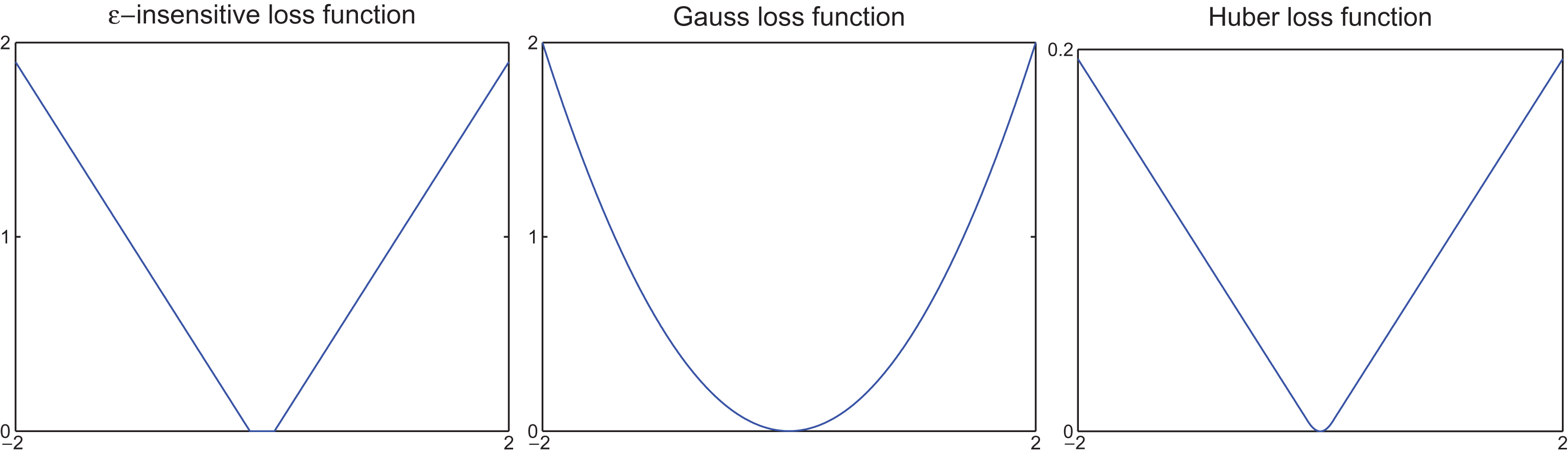
The illustrations of three different loss functions.

3 TSVR with different loss functions

3.1 TSVR with general loss function

Given sample D_l, we construct linear regression function f (x) = w^Tx + b. In the nonlinear case, we map the input vector x_i ∈ R^l into the high dimension feature space with nonlinear mapping. Φ : R^l → H (H is Hibert space). In this case, the inner product of input vector (x_i · x) in feature space is replaced with H (Φ (x_i) · Φ (x_j)). By using kernel function K (·), linear model can be extended to the nonlinear case. $K (x_{i}, x_{j}) = (Φ (x_{i}) \cdot Φ (x_{j})) .$ (15)

First, we conduct uniform TSVR for the different loss functions. We solve the problem based on the general loss function c (ξ) and c (η). Training sample can be written as A = (A₁ ; A₂ ; . . . ; A_n), where A_i = (A_i1, A_i2, . . . , A_in). TSVR mainly achieves the following two functions:

$\begin{matrix} f_{1} (x) & = & K (x^{T}, A^{T}) w_{1} + b_{1}; \\ f_{2} (x) & = & K (x^{T}, A^{T}) w_{2} + b_{2} . \end{matrix}$ (16)

The primal problems of general loss function based TSVR are described as $\begin{matrix} min_{w_{1}, b_{1}, ξ} & \frac{1}{2} (Y - e ɛ_{1} - (K (A, A^{T}) w_{1} + {eb}_{1}))^{T} \\ \times (Y - e ɛ_{1} - (K (A, A^{T}) w_{1} + {eb}_{1})) \\ + C_{1} e^{T} c (ξ) \end{matrix}$ (17) $s . t . Y - (K (A, A^{T}) w_{1} + {eb}_{1}) \geq e ɛ_{1} - ξ, ξ \geq 0,$ and $\begin{matrix} min_{w_{2}, b_{2}, η} & \frac{1}{2} (Y + e ɛ_{2} - (K (A, A^{T}) w_{2} + {eb}_{2}))^{T} \\ \times (Y + e ɛ_{2} - (K (A, A^{T}) w_{2} + {eb}_{2})) \\ + C_{2} e^{T} c (η) \end{matrix}$ (18) $s . t . (K (A, A^{T}) w_{2} + {eb}_{2}) - Y \geq e ɛ_{2} - η, η \geq 0 .$ Where c (ξ) , c (η) are loss functions. C₁, C₂ > 0 are penalty parameters.

3.2 TSVR with ɛ-insensitive loss function

When the loss functions c (ξ_i) = ξ_i, c (η_i) = η_i, the dual problems of TSVR are $\begin{matrix} min_{α} & \frac{1}{2} α^{T} H (H^{T} H)^{- 1} H^{T} α \\ - f^{T} H (H^{T} H)^{- 1} H^{T} α + f^{T} α \end{matrix}$ (19) $s . t . 0 \leq α \leq C_{1} e,$ and $\begin{matrix} min_{γ} & \frac{1}{2} γ^{T} H (H^{T} H)^{- 1} H^{T} γ \\ + h^{T} H (H^{T} H)^{- 1} H^{T} γ - h^{T} γ \end{matrix}$ (20) $s . t . 0 \leq γ \leq C_{2} e .$ where H = [K (A, A^T) e] , f = Y - eɛ₁, h = Y + eɛ₂, and C₁, C₂ > 0 are chosen a priori.

3.3 TSVR with Gaussian loss function

GN-TSVR model for the Gaussian model, Suykens [28], Wu and Law [21, 22] studied the equality and inequality constraints of SVR, respectively. The Gaussian loss functions $c (ξ_{i}) = \frac{ξ_{i}^{2}}{2}$ and $c (η_{i}) = \frac{η_{i}^{2}}{2}$ . The corresponding dual problems are $\begin{matrix} min_{α} & \frac{1}{2} α^{T} H (H^{T} H)^{- 1} H^{T} α - f^{T} H (H^{T} H)^{- 1} H^{T} α \\ + f^{T} α + \frac{1}{2 C_{1}} α^{T} α \end{matrix}$ (21) $s . t . 0 \leq α \leq C_{1} e,$ and $\begin{matrix} min_{γ} & \frac{1}{2} γ^{T} H (H^{T} H)^{- 1} H^{T} γ + h^{T} H (H^{T} H)^{- 1} H^{T} γ \\ - h^{T} γ + \frac{1}{2 C_{2}} γ^{T} γ \end{matrix}$ (22) $s . t . 0 \leq γ \leq C_{2} e .$

It is assumed that the noise obeys standard Gaussian density model. But if the noise obeys Gaussian noise with N (0, σ²), the loss function are $c (ξ_{i}) = \frac{ξ_{i}^{2}}{2 σ^{2}}$ and $c (η_{i}) = \frac{η_{i}^{2}}{2 σ^{2}}$ . Then the dual problems are $\begin{matrix} min_{α} & \frac{1}{2} α^{T} H (H^{T} H)^{- 1} H^{T} α - f^{T} H (H^{T} H)^{- 1} H^{T} α \\ + f^{T} α + \frac{σ^{2}}{2 C_{1}} α^{T} α \end{matrix}$ (23) $s . t . 0 \leq α \leq C_{1} e,$ and $\begin{matrix} min_{γ} & \frac{1}{2} γ^{T} H (H^{T} H)^{- 1} H^{T} γ + h^{T} H (H^{T} H)^{- 1} H^{T} γ \\ - h^{T} γ + \frac{σ^{2}}{2 C_{2}} γ^{T} γ \end{matrix}$ (24) $s . t . 0 \leq γ \leq C_{2} e .$

As we mentioned previously, in real-word applications, the standard Gaussian density model N (0, 1) is commonly used to describe noise. Hence, if no special instructions, GN-TSVR we mentioned uses Equations (21) and (22) in the following experiments.

4 TSVR with Huber loss function

Noticing that it is difficult to deal with the Gaussian noise data with ɛ-insensitive loss function. Thus, Gaussian loss function was proposed. To make further improvements, Huber loss function was proposed based on Gaussian loss function. Combining Equation (14) with TSVR, a novel HN-TSVR is proposed in this section.

HN-TSVR [23 , 29–31] for the Huber model, the Huber loss functions are

$c (ξ_{i}) = {\begin{matrix} \frac{ξ_{i}^{2}}{2}, & if ξ_{i} \leq ɛ, \\ ɛ | ξ_{i} | - \frac{ɛ^{2}}{2}, & otherwise . \end{matrix},$ where $ɛ = ɛ_{1}^{(*)}$ .

Similarly, $c (η_{i}) = {\begin{matrix} \frac{η_{i}^{2}}{2}, & if η_{i} \leq ɛ, \\ ɛ | η_{i} | - \frac{ɛ^{2}}{2}, & otherwise . \end{matrix}$ , where $ɛ = ɛ_{2}^{(*)}$ .

The primal problems of HN-TSVR are $\begin{matrix} min_{w_{1}, b_{1}, ξ} & \frac{1}{2} (Y - e ɛ_{1} - (K (A, A^{T}) w_{1} + {eb}_{1}))^{T} \\ \times (Y - e ɛ_{1} - (K (A, A^{T}) w_{1} + {eb}_{1})) \\ + C_{1} (\sum_{i \in I_{1}} \frac{1}{2} ξ_{i}^{2} + ɛ \sum_{i \in I_{2}} (ξ_{i} - \frac{1}{2} ɛ)) \end{matrix}$ (25) $s . t . Y - (K (A, A^{T}) w_{1} + {eb}_{1}) \geq e ɛ_{1} - ξ, ξ \geq 0,$ where I₁ ={ i|0 ≤ ξ_i < ɛ }, I₂ ={ i|ξ_i ≥ ɛ }.

and $\begin{matrix} min_{w_{2}, b_{2}, η} & \frac{1}{2} (Y + e ɛ_{2} - (K (A, A^{T}) w_{2} + {eb}_{2}))^{T} \\ \times (Y + e ɛ_{2} - (K (A, A^{T}) w_{2} + {eb}_{2})) \\ + C_{2} (\sum_{i \in I_{1}} \frac{1}{2} η_{i}^{2} + ɛ \sum_{i \in I_{2}} (η_{i} - \frac{1}{2} ɛ)) \end{matrix}$ (26) $s . t . (K (A, A^{T}) w_{2} + {eb}_{2}) - Y \geq e ɛ_{2} - η, η \geq 0,$ where I₁ ={ i|0 ≤ η_i < ɛ }, I₂ ={ i|η_i ≥ ɛ }.

We can derive the dual formulations of HN-TSVR as follows, $\begin{matrix} min_{α} & \frac{1}{2} α^{T} H (H^{T} H)^{- 1} H^{T} α - f^{T} H (H^{T} H)^{- 1} H^{T} α \\ + f^{T} α + \frac{1}{2 C_{1}} α^{T} α \end{matrix}$ (27) $s . t . 0 \leq α \leq C_{1} ɛ_{1}^{(*)} e,$ and $\begin{matrix} min_{γ} & \frac{1}{2} γ^{T} H (H^{T} H)^{- 1} H^{T} γ + h^{T} H (H^{T} H)^{- 1} H^{T} γ \\ - h^{T} γ + \frac{1}{2 C_{2}} γ^{T} γ \end{matrix}$ (28) $s . t . 0 \leq γ \leq C_{2} ɛ_{2}^{(*)} e .$

We only derive Equation (27) since Equation (28) is similar to Equation (27). Firstly, we introduce the Lagrange function as

$\begin{matrix} L (w_{1}, b_{1}, ξ, α, β) \\ = \frac{1}{2} (Y - e ɛ_{1} - (K (A, A^{T}) w_{1} + {eb}_{1}))^{T} \\ \times (Y - e ɛ_{1} - (K (A, A^{T}) w_{1} + {eb}_{1})) \\ + C_{1} (\sum_{i \in I_{1}} \frac{1}{2} ξ_{i}^{2} + ɛ \sum_{i \in I_{2}} (ξ_{i} - \frac{1}{2} ɛ)) \\ - α^{T} (Y - (K (A, A^{T}) w_{1} + {eb}_{1}) - e ɛ_{1} + ξ) \\ - β^{T} ξ, \end{matrix}$ (29) where α ≥ 0e, β ≥ 0e are Lagrangian multipliers.

According to KKT conditions, we have $\nabla_{w_{1}} (L) = 0, \nabla_{b_{1}} (L) = 0, \nabla_{ξ} (L) = 0 .$

Then we get $\begin{matrix} - K (A, A^{T})^{T} (Y - K (A, A^{T}) w_{1} - {eb}_{1} - e ɛ_{1}) \\ + K (A, A^{T})^{T} α = 0, \end{matrix}$ (30) $\begin{matrix} - e^{T} (Y - K (A, A^{T}) w_{1} - {eb}_{1} - e ɛ_{1}) \\ + e^{T} α = 0, \end{matrix}$ (31) $C_{1} u_{i} - α_{i} - β_{i} = 0,$ (32)

Where $u_{i} = \frac{\partial (c (ξ_{i}))}{\partial (ξ_{i})} = {\begin{matrix} ξ_{i}, & if i \in I_{1}, \\ ɛ, & if i \in I_{2} . \end{matrix}$ , for i ∈ I₁, we have ξ_i < ɛ, thus, u_i ≤ ɛ. And β_i ≥ 0, then we can get 0 ≤ α_i ≤ C₁u_i. Therefore, we obtain 0 ≤ α_i ≤ C₁ɛ.

Substituting the above KKT conditions into (29), we derive the corresponding dual problem of Equation (25) is $\begin{matrix} min_{α} & \frac{1}{2} α^{T} H (H^{T} H)^{- 1} H^{T} α - f^{T} H (H^{T} H)^{- 1} H^{T} α \\ + f^{T} α + \frac{1}{2 C_{1}} \sum_{i \in I_{1}} α_{i}^{2} + \frac{1}{2} \sum_{i \in I_{2}} C_{1} ɛ^{2} \end{matrix}$ (33) $s . t . 0 \leq α \leq C_{1} ɛ e,$

The following illustrations clarify that Equation (33) is equivalent to Equation (27). Equation (33) can be replaced as

$\begin{matrix} min_{α} & \frac{1}{2} α^{T} H (H^{T} H)^{- 1} H^{T} α - f^{T} H (H^{T} H)^{- 1} H^{T} α \\ + f^{T} α + \frac{1}{2 C_{1}} \sum_{i = 1}^{l} α_{i}^{2} - \frac{1}{2 C_{1}} \sum_{i \in I_{2}} α_{i}^{2} + \frac{C_{1}}{2} \sum_{i \in I_{2}} ɛ^{2} \\ s . t . & 0 \leq α \leq C_{1} ɛ e . \end{matrix}$ (34)

For Equation (34), we introduce the following Lagrange function

$\begin{matrix} L & = & \frac{1}{2} α^{T} H (H^{T} H)^{- 1} H^{T} α - f^{T} H (H^{T} H)^{- 1} H^{T} α \\ + f^{T} α + \frac{1}{2 C_{1}} | | α | |_{2}^{2} + \frac{1}{2} \sum_{i \in I_{2}} C_{1} ɛ^{2} \\ - s^{T} α + γ^{T} (α - C_{1} ɛ e), \end{matrix}$ (35)

According to KKT conditions, there are multiplier γ, δ, let

$\begin{matrix} \frac{\partial L}{\partial α} & = & H (H^{T} H)^{- 1} H^{T} (α - f) + f - s \\ + \frac{1}{C_{1}} δ + γ = 0, \end{matrix}$ (36)

Due to f = Y - eɛ₁, we can transform Equation (36) into

$\begin{matrix} \frac{\partial L}{\partial α} & = & H (H^{T} H)^{- 1} H^{T} (α - f) + Y - e ɛ_{1} - s \\ + \frac{1}{C_{1}} δ + γ = 0, \end{matrix}$ (37) where s, γ ≥ 0, and $δ_{i} = {\begin{matrix} α_{i}, & if i \in I_{1}, \\ 0, & if i \in I_{2} . \end{matrix}$ .

Let $ξ = γ + \frac{1}{C_{1}} δ$ , according to Equation (37), we have $H (H^{T} H)^{- 1} H^{T} (α - f) + Y \leq e ɛ_{1} - ξ,$ (38)

Put $u_{1} = [w_{1}^{T} b_{1}]^{T} = (H^{T} H)^{- 1} H^{T} (f - α)$ into Equation (38), we get $Y - (K (A, A^{T}) w_{1} + {eb}_{1}) \geq e ɛ_{1} - ξ,$ (39) where ξ ≥ 0 is the slack variable of primal problem. And if i ∈ I₁, ξ_i < ɛ, we will get 0 ≤ α_i < C₁ɛ. And if i ∈ I₂, ξ_i ≥ ɛ, we will have α_i = C₁ɛ, otherwise δ = 0 or γ = 0, which will cause ξ_i < ɛ. And it is contradictory with ξ_i ≥ ɛ. Therefore, for all i ∈ I₂, there must have α_i = C₁ɛ. According to these, we have $\begin{matrix} \frac{1}{2 C_{1}} \sum_{i \in I_{2}} (α_{i})^{2} - \frac{1}{2} C_{1} \sum_{i \in I_{2}} ɛ^{2} \\ = \frac{1}{2 C_{1}} \sum_{i \in I_{2}} (C_{1} ɛ)^{2} - \frac{1}{2} C_{1} \sum_{i \in I_{2}} ɛ^{2} = 0 . \end{matrix}$ Therefore the last two terms in the objective function (34) are equal to zero. So Equation (33) is equivalent to Equation (27).

5 Experiments and discussion

To demonstrate the validity of the proposed TSVR with Huber loss function, we compared it with TSVR and TSVR with Gaussian loss function on a collection of datasets, including artificial datasets, nine benchmark datasets with Gaussian noise and financial time series dataset.

The performance of these algorithms depend on the collection of parameters. In our experiments, we set $C_{1} = C_{2}, ɛ_{1} = ɛ_{2}, ɛ_{1}^{(*)} = ɛ_{2}^{(*)}$ to degrade the computational complexity of parameter selection. In order to evaluate the performance of different algorithms, the evaluation criteria are specified before experiments. Let l be the number of test sample, y_i and $\hat{y_{i}}$ is the real value and predicted value of sample x_i, respectively. Demonstrate $\bar{y}$ as the average value of y₁, y₂, ⋯ , y_l. We use the following evaluation criteria [18 , 33].

MAE: Mean absolute error, which is defined as $MAE = \frac{1}{l} \sum_{i = 1}^{l} | \hat{y_{i}} - y_{i} |$ . MAE is used to evaluate the deviation measurement of real value and predicted value.

RMSE: Root mean squared error, which is defined as $RMSE = \sqrt{\frac{1}{l} \sum_{i = 1}^{l} (\hat{y_{i}} - y_{i})^{2}}$ . It is also commonly used the deviation measurement of real value and predicted value.

SSE/SST: Ratio between sum squared error $SSE = \frac{1}{l} \sum_{i = 1}^{l} (\hat{y_{i}} - \bar{y})^{2}$ and the sum squared deviation of testing samples $SST = \sum_{i = 1}^{l} (y_{i} - \bar{y})^{2}$ . SSE represents fitting precision. The smaller SSE is, the fitter the estimation is. However, when noises are also used as testing samples, too small value of SSE probably speaks for overfitting of regressor. SST reflects the underlying variance of the testing samples.

SSR/SST: Ratio between interpretable sum squared deviation $SSR = \sum_{i = 1}^{l} (\hat{y_{i}} - \bar{y})^{2}$ and SST. SSR reflects the explanation ability of the regressor.

In most cases, small SSE/SST means good agreement between estimations and real values, and to obtain smaller SSE/SST usually accompanies an increase of SSR/SST. However, the extremely small value of SSE/SST is in fact not good, for it probably means overfitting of the regressor. Therefore, a good estimator should strike balance between SSE/SST and SSR/SST.

In this section, we use Gaussian kernel function to evaluate TSVR, GN-TSVR and HN-TSVR. $\begin{matrix} K (x_{i}, x_{j}) = e^{- \frac{∥ x_{i} - x_{j} ∥^{2}}{p^{2}}} \end{matrix}$

It is well known that the performances of algorithms depend on the choice of parameters. The optimal values of the parameters were determined by applying five-fold cross validation [32, 34]. The optimal parameter C in each algorithm was searched from set {2ⁱ|i = -3, - 2, - 1, 0, ⋯ , 8}. The optimal parameter ɛ₁, ɛ₂ was chosen from set ${\frac{i}{10} | i = 1, 2, \dots, 9}$ . The optimal p was selected over the range {2ⁱ|i = -4, ⋯ , 8}. The optimal parameter $ɛ_{1}^{(*)}, ɛ_{2}^{(*)}$ was chosen from set ${\frac{i}{10} | i = 1, 3, 5, 7, 9}$ .

5.1 Artificial datasets

The regressions of sinc function $y = \frac{sin π x}{π x}, x \in [- 6, 6]$ were tested to verify the performance of the HN-TSVR. Training data points were perturbed by Gaussian noises. Specially, the following kinds of training samples (x_i, y_i) , i = 1, ⋯ , n were generated

$\begin{matrix} y_{i} = \frac{sin π x_{i}}{π x_{i}} + η_{i}, \\ x \sim U [- 6, 6], η_{i} \sim N (0, 0 . 15^{2}), \end{matrix}$ (40)

$\begin{matrix} y_{i} = \frac{sin π x_{i}}{π x_{i}} + η_{i}, \\ x \sim U [- 6, 6], η_{i} \sim N (0, 1^{2}), \end{matrix}$ (41) where N (0, d²) represents the Gaussian random variable with zero mean and variance d².

In order to avoid of biased comparisons, we randomly generated ten independent groups of noisy samples which respectively consists of 150 training samples and 150 test samples. The test data are uniformly sampled from the objective sinc function without any noise. The comparisons of experimental results are summarized in Table 1.

Table 1

Performance comparisons of three algorithms on Sinc with Gaussian noise

Datasets	Regressor	MAE	RMSE	SSE/SST	SSR/SST
Type 0.15	TSVR	0.040378 ± 0.005736	0.050841 ± 0.007288	0.044137 ± 0.025063	0.980006 ± 0.090619
	GN-TSVR	0.040420 ± 0.005959	0.050706 ± 0.006986	0.042565 ± 0.020810	0.976295 ± 0.067012
	HN-TSVR	0.040199 ± 0.004682	0.050605 ± 0.007206	0.042459 ± 0.021325	0.973707 ± 0.066786
Type 1	TSVR	0.244683 ± 0.056423	0.310921 ± 0.062322	1.553032 ± 0.788761	1.062383 ± 0.6211387
	GN-TSVR	0.241183 ± 0.037190	0.291416 ± 0.052218	1.433215 ± 0.758312	1.456029 ± 0.448091
	HN-TSVR	0.239680 ± 0.037443	0.289017 ± 0.052682	1.412628 ± 0.747213	1.440943 ± 0.431146

From Table 1, we can find that the HN-TSVR yields lightly lower regression error compared with TSVR and GN-TSVR. When the noise obeys N (0, 1), we find that the GN-TSVR is better than TSVR. However, when the noise obeys N (0, 0 . 15²), we find that the performance of TSVR is better than GN-TSVR. In Section 3.3, GN-TSVR uses Equations (21) and (22). However, according to the experimental results, when the noise obeys N (0, 0 . 15²), if we use Equations (21) and (22), the performance of TSVR is better than GN-TSVR. Thus, according to the discussion of Section 3.3, if the noise obeys N (0, d²), we should fix σ = d and then GN-TSVR can get the best performance. Now for GN-TSVR we use the Equations (23) and (24) which noise obeys N (0, 0 . 15²), that is to say, we fix the σ = 0.15 in Equations (23) and (24). We want to compare TSVR, changed GN-TSVR and HN-TSVR, then we get Table 2.

Table 2

Performance comparisons of TSVR, changed GN-TSVR and HN-TSVR on Sinc dataset with Gaussian noise

Datasets	Regressor	MAE	RMSE	SSE/SST	SSR/SST
Type 0.15	TSVR	0.040378 ± 0.005736	0.050841 ± 0.007288	0.044137 ± 0.025063	0.980006 ± 0.090619
	GN-TSVR	0.040275 ± 0.005588	0.051261 ± 0.007574	0.045189 ± 0.026473	0.980411 ± 0.085518
	HN-TSVR	0.040199 ± 0.004682	0.050605 ± 0.007206	0.042459 ± 0.021325	0.973707 ± 0.066786

We can get changed GN-TSVR is better than TSVR, but HN-TSVR still obtains the smallest MAE and RMSE among three algorithms for two types of Gaussian noise.

From Tables 1 and 2, we can find that GN-TSVR, HN-TSVR are better than TSVR on the artificial datasets. Besides, HN-TSVR is better than GN-TSVR. And for different noise model, HN-TSVR has universality.

For the following experiments, we mainly discuss the case of noise data with variance one for the reason that the standard Gaussian density model N (0, 1) is commonly used to describe noise in real-world applications.

Curve sinc and fitting curves obtained by TSVR, GN-TSVR, HN-TSVR are illustrated in Fig. 2.

Fig.2

Curve sinc and fitting curves obtained by TSVR, GN-TSVR, HN-TSVR.

5.2 Nine benchmark datasets

In this section, we use Chwirut, Cons, Bodyfat, Diabetes, Auto Mpg, Ozone, Pyrim, Triazines, Wisconsin Breast Cancer (Wis. BC) from the UCI machine learning repository 1 to test TSVR, GN-TSVR and HN-TSVR. We evaluate three algorithms by four estimation criteria: RMSE, MAE, SSE/SST, SSR/SST. The comparisons of experimental results are summarized in Table 3.

Table 3
Performance comparisons of three algorithms on benchmark datasets with Gaussian kernel function

Datasets Regressor MAE RMSE SSE/SST SSR/SST

Chwirut TSVR 0.028115 ± 0.012395 0.038495 ± 0.017086 0.024090 ± 0.016850 1.013226 ± 0.136349

(214×1) GN-TSVR 0.028662 ± 0.011770 0.039083 ± 0.016601 0.024628 ± 0.016514 1.014396 ± 0.139633

HN-TSVR 0.028641 ± 0.011817 0.039061 ± 0.016633 0.024614 ± 0.016539 1.014177 ± 0.139647

Cons TSVR 0.183330 ± 0.025964 0.220667 ± 0.020969 0.613684 ± 0.219460 0.446074 ± 0.259974

(103×7) GN-TSVR 0.184413 ± 0.025853 0.220738 ± 0.020295 0.612165 ± 0.211481 0.440647 ± 0.270926

HN-TSVR 0.183424 ± 0.025356 0.221546 ± 0.019573 0.617052 ± 0.215351 0.460014 ± 0.296884

Bodyfat TSVR 0.074084 ± 0.008403 0.092314 ± 0.010741 0.362778 ± 0.167116 0.742342 ± 0.255449

(252×13) GN-TSVR 0.074767 ± 0.007881 0.093347 ± 0.010384 0.370952 ± 0.170795 0.750733 ± 0.282130

HN-TSVR 0.074449 ± 0.008121 0.092940 ± 0.010485 0.366376 ± 0.164180 0.745745 ± 0.272904

Diabetes TSVR 0.477039 ± 0.078531 0.625350 ± 0.071612 1.032078 ± 0.427042 0.694044 ± 0.368162

(43×3) GN-TSVR 0.488680 ± 0.101804 0.605023 ± 0.064749 0.986584 ± 0.454362 0.691839 ± 0.470468

HN-TSVR 0.476482 ± 0.071326 0.619507 ± 0.067719 1.001380 ± 0.366886 0.630942 ± 0.302050

Auto MPG TSVR 2.818329 ± 0.338631 3.889705 ± 0.337473 0.253304 ± 0.045947 0.800710 ± 0.122437

(392×8) GN-TSVR 2.825014 ± 0.353941 3.881589 ± 0.358300 0.252316 ± 0.047151 0.798222 ± 0.127844

HN-TSVR 2.825014 ± 0.353941 3.881589 ± 0.358300 0.252316 ± 0.047151 0.798222 ± 0.127844

Ozone TSVR 13.79415 ± 2.459491 19.00365 ± 6.506568 0.343636 ± 0.143970 0.647899 ± 0.226621

(111×4) GN-TSVR 13.80225 ± 2.461076 19.01831 ± 6.517456 0.344123 ± 0.144242 0.646428 ± 0.224016

HN-TSVR 13.78085 ± 2.507963 19.00922 ± 6.556569 0.343972 ± 0.145668 0.636644 ± 0.211815

Pyrim TSVR 0.048159 ± 0.010200 0.068463 ± 0.029307 0.297521 ± 0.116855 0.854406 ± 0.391961

(74×28) GN-TSVR 0.048817 ± 0.009991 0.068695 ± 0.028819 0.299488 ± 0.112969 0.846886 ± 0.388372

HN-TSVR 0.048816 ± 0.009991 0.068695 ± 0.028823 0.299490 ± 0.113010 0.846894 ± 0.388399

Triazines TSVR 0.098359 ± 0.014446 0.133669 ± 0.023659 0.739624 ± 0.185246 0.365725 ± 0.123771

(186×61) GN-TSVR 0.100414 ± 0.012418 0.133999 ± 0.020989 0.741652 ± 0.154162 0.365194 ± 0.121973

HN-TSVR 0.098860 ± 0.013120 0.133257 ± 0.022024 0.734220 ± 0.166803 0.368001 ± 0.121348

Wis.BC TSVR 28.13674 ± 4.109204 34.10531 ± 4.623342 1.043355 ± 0.192108 0.352460 ± 0.109560

(194×33) GN-TSVR 28.18037 ± 4.066262 34.13888 ± 4.563274 1.045983 ± 0.193558 0.350863 ± 0.111333

HN-TSVR 27.95632 ± 4.324383 34.07242 ± 4.698815 1.039971 ± 0.186025 0.360635 ± 0.096328

Datasets	Regressor	MAE	RMSE	SSE/SST	SSR/SST
Chwirut	TSVR	0.028115 ± 0.012395	0.038495 ± 0.017086	0.024090 ± 0.016850	1.013226 ± 0.136349
(214×1)	GN-TSVR	0.028662 ± 0.011770	0.039083 ± 0.016601	0.024628 ± 0.016514	1.014396 ± 0.139633
	HN-TSVR	0.028641 ± 0.011817	0.039061 ± 0.016633	0.024614 ± 0.016539	1.014177 ± 0.139647
Cons	TSVR	0.183330 ± 0.025964	0.220667 ± 0.020969	0.613684 ± 0.219460	0.446074 ± 0.259974
(103×7)	GN-TSVR	0.184413 ± 0.025853	0.220738 ± 0.020295	0.612165 ± 0.211481	0.440647 ± 0.270926
	HN-TSVR	0.183424 ± 0.025356	0.221546 ± 0.019573	0.617052 ± 0.215351	0.460014 ± 0.296884
Bodyfat	TSVR	0.074084 ± 0.008403	0.092314 ± 0.010741	0.362778 ± 0.167116	0.742342 ± 0.255449
(252×13)	GN-TSVR	0.074767 ± 0.007881	0.093347 ± 0.010384	0.370952 ± 0.170795	0.750733 ± 0.282130
	HN-TSVR	0.074449 ± 0.008121	0.092940 ± 0.010485	0.366376 ± 0.164180	0.745745 ± 0.272904
Diabetes	TSVR	0.477039 ± 0.078531	0.625350 ± 0.071612	1.032078 ± 0.427042	0.694044 ± 0.368162
(43×3)	GN-TSVR	0.488680 ± 0.101804	0.605023 ± 0.064749	0.986584 ± 0.454362	0.691839 ± 0.470468
	HN-TSVR	0.476482 ± 0.071326	0.619507 ± 0.067719	1.001380 ± 0.366886	0.630942 ± 0.302050
Auto MPG	TSVR	2.818329 ± 0.338631	3.889705 ± 0.337473	0.253304 ± 0.045947	0.800710 ± 0.122437
(392×8)	GN-TSVR	2.825014 ± 0.353941	3.881589 ± 0.358300	0.252316 ± 0.047151	0.798222 ± 0.127844
	HN-TSVR	2.825014 ± 0.353941	3.881589 ± 0.358300	0.252316 ± 0.047151	0.798222 ± 0.127844
Ozone	TSVR	13.79415 ± 2.459491	19.00365 ± 6.506568	0.343636 ± 0.143970	0.647899 ± 0.226621
(111×4)	GN-TSVR	13.80225 ± 2.461076	19.01831 ± 6.517456	0.344123 ± 0.144242	0.646428 ± 0.224016
	HN-TSVR	13.78085 ± 2.507963	19.00922 ± 6.556569	0.343972 ± 0.145668	0.636644 ± 0.211815
Pyrim	TSVR	0.048159 ± 0.010200	0.068463 ± 0.029307	0.297521 ± 0.116855	0.854406 ± 0.391961
(74×28)	GN-TSVR	0.048817 ± 0.009991	0.068695 ± 0.028819	0.299488 ± 0.112969	0.846886 ± 0.388372
	HN-TSVR	0.048816 ± 0.009991	0.068695 ± 0.028823	0.299490 ± 0.113010	0.846894 ± 0.388399
Triazines	TSVR	0.098359 ± 0.014446	0.133669 ± 0.023659	0.739624 ± 0.185246	0.365725 ± 0.123771
(186×61)	GN-TSVR	0.100414 ± 0.012418	0.133999 ± 0.020989	0.741652 ± 0.154162	0.365194 ± 0.121973
	HN-TSVR	0.098860 ± 0.013120	0.133257 ± 0.022024	0.734220 ± 0.166803	0.368001 ± 0.121348
Wis.BC	TSVR	28.13674 ± 4.109204	34.10531 ± 4.623342	1.043355 ± 0.192108	0.352460 ± 0.109560
(194×33)	GN-TSVR	28.18037 ± 4.066262	34.13888 ± 4.563274	1.045983 ± 0.193558	0.350863 ± 0.111333
	HN-TSVR	27.95632 ± 4.324383	34.07242 ± 4.698815	1.039971 ± 0.186025	0.360635 ± 0.096328

From Table 3 we can discover that TSVR yields better performance than GN-TSVR and HN-TSVR for most cases. But TSVR does not outperform other two algorithms in all datasets. In order to further evaluate, Table 4 shows the average rank of three algorithms. From it we can get the average rank of TSVR is far lower than GN-TSVR and lightly lower than HN-TSVR. That is to say, it is not suitable to apply algorithms with Gaussian loss and Huber loss to the data with non-Gaussian noise.

Table 4

Average ranks of TSVR, GN-TSVR, HN-TSVR on MAE values

Datasets	TSVR	GN-TSVR	HN-TSVR
Chwirut	1	3	2
Cons	1	3	2
Bodyfat	1	3	2
Diabetes	2	3	1
Auto MPG	1	2.5	2.5
Ozone	2	3	1
Pyrim	1	3	2
Triazines	1	3	2
Wis.BC	2	3	1
Average rank	1.33	2.94	1.72

5.3 Nine benchmark datasets with Gaussian noise

From above discussion, we know it is not suitable to apply algorithms with Gaussian loss and Huber loss to the benchmark datasets with non-Gaussian noise. Therefore, in this section, we add Gaussian noise to nine benchmark datasets and compare the performance of three models in order to further illustrate that Gaussian noise affects the performance of three models. The validity of our proposed algorithm is also demonstrated using nine benchmark datasets with Gaussian noise.

For the nine benchmark datasets, we divide each datasets into training samples and test samples. Every training samples with Gaussian noise, and every test training samples with no noise. The comparisons of TSVR, GN-TSVR,HN-TSVR on benchmark datasets with Gaussian noise are summarized in Table 5. In error items, the first item denotes the mean value of five times testing results, and the second item stands for plus or minus the standard deviation.

Table 5
Performance comparisons of three algorithms on benchmark datasets with Gaussian noise

Datasets Regressor MAE RMSE SSE/SST SSR/SST

Chwirut TSVR 0.120106 ± 0.031277 0.157950 ± 0.039165 0.362185 ± 0.192923 1.463683 ± 0.354368

(214×1) GN-TSVR 0.124217 ± 0.025944 0.164376 ± 0.035037 0.388350 ± 0.178674 1.469748 ± 0.347723

HN-TSVR 0.121195 ± 0.030647 0.154826 ± 0.035103 0.343133 ± 0.166780 1.465055 ± 0.334262

Cons TSVR 0.235648 ± 0.044208 0.300896 ± 0.040101 1.057967 ± 0.085123 0.106717 ± 0.092190

(103×7) GN-TSVR 0.232627 ± 0.044195 0.321382 ± 0.034294 1.218788 ± 0.172354 0.251873 ± 0.141596

HN-TSVR 0.230680 ± 0.038432 0.299361 ± 0.035482 1.052681 ± 0.124538 0.105406 ± 0.081421

Bodyfat TSVR 0.187301 ± 0.048079 0.217541 ± 0.050606 1.829458 ± 0.722419 1.685472 ± 0.824394

(252×13) GN-TSVR 0.180138 ± 0.063556 0.213507 ± 0.067838 1.943384 ± 1.336000 2.124196 ± 1.456861

HN-TSVR 0.180138 ± 0.063556 0.213507 ± 0.067838 1.943384 ± 1.336000 2.124196 ± 1.456861

Diabetes TSVR 0.419510 ± 0.129826 0.521554 ± 0.176960 1.517659 ± 1.056077 1.056231 ± 1.132908

(43×3) GN-TSVR 0.412388 ± 0.155622 0.516089 ± 0.201828 1.402437 ± 0.855213 0.960814 ± 0.809263

HN-TSVR 0.409692 ± 0.156196 0.513912 ± 0.199948 1.362576 ± 0.748707 0.905377 ± 0.768824

Auto MPG TSVR 2.809569 ± 0.343873 3.713372 ± 0.395648 0.233962 ± 0.036899 0.760471 ± 0.072846

(392×8) GN-TSVR 2.801230 ± 0.299592 3.719405 ± 0.396712 0.235146 ± 0.040579 0.764582 ± 0.073402

HN-TSVR 2.800798 ± 0.287945 3.715329 ± 0.387381 0.234648 ± 0.039909 0.764037 ± 0.073917

Ozone TSVR 16.47019 ± 6.834435 22.33604 ± 10.49242 0.483843 ± 0.249515 0.768761 ± 0.395904

(111×4) GN-TSVR 16.48578 ± 6.898186 22.32140 ± 10.50765 0.483150 ± 0.249824 0.765565 ± 0.394654

HN-TSVR 16.47118 ± 6.863079 22.33534 ± 10.51571 0.483851 ± 0.249859 0.764606 ± 0.395684

Pyrim TSVR 0.099161 ± 0.065556 0.130242 ± 0.091998 1.556402 ± 0.850769 0.556221 ± 0.850754

(74×28) GN-TSVR 0.098994 ± 0.060660 0.131310 ± 0.087315 1.672150 ± 0.695249 0.671948 ± 0.695120

HN-TSVR 0.098994 ± 0.060660 0.131310 ± 0.087315 1.672150 ± 0.695249 0.671948 ± 0.695120

Triazines TSVR 0.127091 ± 0.024484 0.174348 ± 0.039901 1.161839 ± 0.196979 0.179549 ± 0.199873

(186×61) GN-TSVR 0.126736 ± 0.026544 0.171994 ± 0.041057 1.129446 ± 0.219887 0.137346 ± 0.221873

HN-TSVR 0.126524 ± 0.024794 0.171619 ± 0.039067 1.125583 ± 0.185720 0.137557 ± 0.188398

Wis.BC TSVR 29.31731 ± 4.466406 34.34753 ± 4.643696 1.152692 ± 0.306474 0.225922 ± 0.272325

(194×33) GN-TSVR 29.31735 ± 4.466433 34.34753 ± 4.643718 1.152692 ± 0.306471 0.225920 ± 0.272324

HN-TSVR 29.31735 ± 4.466433 34.34753 ± 4.643718 1.152692 ± 0.306471 0.225920 ± 0.272324

Datasets	Regressor	MAE	RMSE	SSE/SST	SSR/SST
Chwirut	TSVR	0.120106 ± 0.031277	0.157950 ± 0.039165	0.362185 ± 0.192923	1.463683 ± 0.354368
(214×1)	GN-TSVR	0.124217 ± 0.025944	0.164376 ± 0.035037	0.388350 ± 0.178674	1.469748 ± 0.347723
	HN-TSVR	0.121195 ± 0.030647	0.154826 ± 0.035103	0.343133 ± 0.166780	1.465055 ± 0.334262
Cons	TSVR	0.235648 ± 0.044208	0.300896 ± 0.040101	1.057967 ± 0.085123	0.106717 ± 0.092190
(103×7)	GN-TSVR	0.232627 ± 0.044195	0.321382 ± 0.034294	1.218788 ± 0.172354	0.251873 ± 0.141596
	HN-TSVR	0.230680 ± 0.038432	0.299361 ± 0.035482	1.052681 ± 0.124538	0.105406 ± 0.081421
Bodyfat	TSVR	0.187301 ± 0.048079	0.217541 ± 0.050606	1.829458 ± 0.722419	1.685472 ± 0.824394
(252×13)	GN-TSVR	0.180138 ± 0.063556	0.213507 ± 0.067838	1.943384 ± 1.336000	2.124196 ± 1.456861
	HN-TSVR	0.180138 ± 0.063556	0.213507 ± 0.067838	1.943384 ± 1.336000	2.124196 ± 1.456861
Diabetes	TSVR	0.419510 ± 0.129826	0.521554 ± 0.176960	1.517659 ± 1.056077	1.056231 ± 1.132908
(43×3)	GN-TSVR	0.412388 ± 0.155622	0.516089 ± 0.201828	1.402437 ± 0.855213	0.960814 ± 0.809263
	HN-TSVR	0.409692 ± 0.156196	0.513912 ± 0.199948	1.362576 ± 0.748707	0.905377 ± 0.768824
Auto MPG	TSVR	2.809569 ± 0.343873	3.713372 ± 0.395648	0.233962 ± 0.036899	0.760471 ± 0.072846
(392×8)	GN-TSVR	2.801230 ± 0.299592	3.719405 ± 0.396712	0.235146 ± 0.040579	0.764582 ± 0.073402
	HN-TSVR	2.800798 ± 0.287945	3.715329 ± 0.387381	0.234648 ± 0.039909	0.764037 ± 0.073917
Ozone	TSVR	16.47019 ± 6.834435	22.33604 ± 10.49242	0.483843 ± 0.249515	0.768761 ± 0.395904
(111×4)	GN-TSVR	16.48578 ± 6.898186	22.32140 ± 10.50765	0.483150 ± 0.249824	0.765565 ± 0.394654
	HN-TSVR	16.47118 ± 6.863079	22.33534 ± 10.51571	0.483851 ± 0.249859	0.764606 ± 0.395684
Pyrim	TSVR	0.099161 ± 0.065556	0.130242 ± 0.091998	1.556402 ± 0.850769	0.556221 ± 0.850754
(74×28)	GN-TSVR	0.098994 ± 0.060660	0.131310 ± 0.087315	1.672150 ± 0.695249	0.671948 ± 0.695120
	HN-TSVR	0.098994 ± 0.060660	0.131310 ± 0.087315	1.672150 ± 0.695249	0.671948 ± 0.695120
Triazines	TSVR	0.127091 ± 0.024484	0.174348 ± 0.039901	1.161839 ± 0.196979	0.179549 ± 0.199873
(186×61)	GN-TSVR	0.126736 ± 0.026544	0.171994 ± 0.041057	1.129446 ± 0.219887	0.137346 ± 0.221873
	HN-TSVR	0.126524 ± 0.024794	0.171619 ± 0.039067	1.125583 ± 0.185720	0.137557 ± 0.188398
Wis.BC	TSVR	29.31731 ± 4.466406	34.34753 ± 4.643696	1.152692 ± 0.306474	0.225922 ± 0.272325
(194×33)	GN-TSVR	29.31735 ± 4.466433	34.34753 ± 4.643718	1.152692 ± 0.306471	0.225920 ± 0.272324
	HN-TSVR	29.31735 ± 4.466433	34.34753 ± 4.643718	1.152692 ± 0.306471	0.225920 ± 0.272324

Table 5 shows the testing results of our proposed HN-TSVR, TSVR and GN-TSVR on nine benchmark datasets with Gaussian noise. We compare estimation criteria and we can see that except that MAE of TSVR on Chwirut, Ozone, Wis. BC are far lower than that of GN-TSVR and lightly lower than HN-TSVR, all the other testing errors of HN-TSVR are lower than TSVR and GN-TSVR. Otherwise, MAE of TSVR are far lower than that of GN-TSVR and lightly lower than HN-TSVR on above six datasets with no Gaussian noise. That is to say, HN-TSVR is better than TSVR and GN-TSVR for most datasets. Meanwhile we can see that our proposed HN-TSVR does not outperform other two algorithms on all datasets. Therefore, in order to further evaluate three algorithms, the average ranks are shown in Table 6, from it we can find that the average rank of HN-TSVR is lower than that of TSVR and GN-TSVR. It implies that our proposed HN-TSVR is better than other two algorithms.

Table 6

Average ranks of TSVR, GN-TSVR, HN-TSVR on MAE values

Datasets	TSVR	GN-TSVR	HN-TSVR
Chwirut	1	3	2
Cons	3	2	1
Bodyfat	3	1.5	1.5
Diabetes	3	2	1
Auto MPG	3	2	1
Ozone	1	3	2
Pyrim	3	1.5	1.5
Triazines	3	2	1
Wis.BC	1	2.5	2.5
Average rank	2.27	2.22	1.5

5.4 Financial time series dataset

In order to further check the validity of our proposed HN-TSVR, the financial time series dataset is analyzed in this section. The data of financial time series is random, which is usually high noisy and contains strong nonlinearity and outliers. And for Shanghai Stock Exchange Composite Index (SSECI) 2 , it has strong randomness since there are many influence factors. It is assumed that the influence factors of the closing price are decided by the day before the opening price (yuan), the closing price (yuan), the highest price (yuan), the lowest price (yuan), trading volume (share), volume of business (yuan). We also employ five-fold cross validation to evaluate the performance of algorithms. That is to say, the dataset is split randomly into five subsets, and one of those sets is reserved as a test set; this process is repeated five times. The comparisons of TSVR, GN-TSVR, HN-TSVR on financial time series dataset are summarized in Table 7.

Table 7
Performance comparisons of three algorithms on financial time series dataset

Datasets Regressor MAE RMSE SSE/SST SSR/SST

SSECI-2010 TSVR 31.12659 ± 10.80883 40.58929 ± 14.12458 0.034323 ± 0.021277 0.950324 ± 0.076450

GN-TSVR 31.11639 ± 10.85779 40.59933 ± 14.18642 0.034376 ± 0.021397 0.950599 ± 0.070979

HN-TSVR 31.11130 ± 10.87291 40.64443 ± 40.64443 0.034410 ± 0.021283 0.948368 ± 0.070979

SSECI-2011 TSVR 25.71714 ± 4.263458 30.92483 ± 4.222643 0.017493 ± 0.006150 0.993889 ± 0.065989

GN-TSVR 25.71095 ± 4.257972 30.92600 ± 4.208778 0.017477 ± 0.006070 0.993802 ± 0.065495

HN-TSVR 25.66553 ± 4.536392 30.90966 ± 4.403136 0.017477 ± 0.006178 0.996409 ± 0.069302

SSECI-2012 TSVR 18.47599 ± 1.439796 24.05766 ± 1.776894 0.031032 ± 0.005169 0.959539 ± 0.025308

GN-TSVR 18.46431 ± 1.424920 24.03442 ± 1.794099 0.030975 ± 0.005197 0.959351 ± 0.025516

HN-TSVR 18.41835 ± 1.397594 24.04776 ± 1.582303 0.030988 ± 0.004778 0.960433 ± 0.024203

SSECI-2013 TSVR 23.19700 ± 5.246675 31.34839 ± 5.024618 0.088474 ± 0.030420 0.871714 ± 0.130008

GN-TSVR 23.20194 ± 5.282049 31.34984 ± 5.048097 0.088453 ± 0.030430 0.872625 ± 0.130384

HN-TSVR 23.20194 ± 5.282049 31.34984 ± 5.048097 0.088453 ± 0.030430 0.872625 ± 0.130384

SSECI-2014 TSVR 22.96096 ± 4.520105 32.12406 ± 6.918126 0.013075 ± 0.003702 0.903067 ± 0.053237

GN-TSVR 22.95612 ± 4.536574 32.11805 ± 6.950670 0.013075 ± 0.003743 0.903645 ± 0.053753

HN-TSVR 22.71593 ± 4.797966 32.02347 ± 7.153597 0.013081 ± 0.004270 0.909327 ± 0.057875

SSECI-2015 TSVR 75.98378 ± 15.46194 104.0880 ± 20.86282 0.044486 ± 0.020041 0.940123 ± 0.096697

GN-TSVR 75.96272 ± 15.52842 104.0537 ± 20.94753 0.044441 ± 0.020006 0.940097 ± 0.096977

HN-TSVR 75.96272 ± 15.52842 104.0537 ± 20.94753 0.044441 ± 0.020006 0.940097 ± 0.096977

Datasets	Regressor	MAE	RMSE	SSE/SST	SSR/SST
SSECI-2010	TSVR	31.12659 ± 10.80883	40.58929 ± 14.12458	0.034323 ± 0.021277	0.950324 ± 0.076450
	GN-TSVR	31.11639 ± 10.85779	40.59933 ± 14.18642	0.034376 ± 0.021397	0.950599 ± 0.070979
	HN-TSVR	31.11130 ± 10.87291	40.64443 ± 40.64443	0.034410 ± 0.021283	0.948368 ± 0.070979
SSECI-2011	TSVR	25.71714 ± 4.263458	30.92483 ± 4.222643	0.017493 ± 0.006150	0.993889 ± 0.065989
	GN-TSVR	25.71095 ± 4.257972	30.92600 ± 4.208778	0.017477 ± 0.006070	0.993802 ± 0.065495
	HN-TSVR	25.66553 ± 4.536392	30.90966 ± 4.403136	0.017477 ± 0.006178	0.996409 ± 0.069302
SSECI-2012	TSVR	18.47599 ± 1.439796	24.05766 ± 1.776894	0.031032 ± 0.005169	0.959539 ± 0.025308
	GN-TSVR	18.46431 ± 1.424920	24.03442 ± 1.794099	0.030975 ± 0.005197	0.959351 ± 0.025516
	HN-TSVR	18.41835 ± 1.397594	24.04776 ± 1.582303	0.030988 ± 0.004778	0.960433 ± 0.024203
SSECI-2013	TSVR	23.19700 ± 5.246675	31.34839 ± 5.024618	0.088474 ± 0.030420	0.871714 ± 0.130008
	GN-TSVR	23.20194 ± 5.282049	31.34984 ± 5.048097	0.088453 ± 0.030430	0.872625 ± 0.130384
	HN-TSVR	23.20194 ± 5.282049	31.34984 ± 5.048097	0.088453 ± 0.030430	0.872625 ± 0.130384
SSECI-2014	TSVR	22.96096 ± 4.520105	32.12406 ± 6.918126	0.013075 ± 0.003702	0.903067 ± 0.053237
	GN-TSVR	22.95612 ± 4.536574	32.11805 ± 6.950670	0.013075 ± 0.003743	0.903645 ± 0.053753
	HN-TSVR	22.71593 ± 4.797966	32.02347 ± 7.153597	0.013081 ± 0.004270	0.909327 ± 0.057875
SSECI-2015	TSVR	75.98378 ± 15.46194	104.0880 ± 20.86282	0.044486 ± 0.020041	0.940123 ± 0.096697
	GN-TSVR	75.96272 ± 15.52842	104.0537 ± 20.94753	0.044441 ± 0.020006	0.940097 ± 0.096977
	HN-TSVR	75.96272 ± 15.52842	104.0537 ± 20.94753	0.044441 ± 0.020006	0.940097 ± 0.096977

From Table 7, we can get only for SSECI-2013 in the near six years SSECI we selected, TSVR is better than GN-TSVR and HN-TSVR. However, for other datasets, it has been seen that our HN-TSVR obviously outperforms other two models. To further evaluate three algorithms, the average ranks are shown in Table 8.

Table 8

Average ranks of TSVR, GN-TSVR, HN-TSVR on MAE values

Datasets	TSVR	GN-TSVR	HN-TSVR
SSECI-2010	3	2	1
SSECI-2011	3	2	1
SSECI-2012	3	2	1
SSECI-2013	1	2.5	2.5
SSECI-2014	3	2	1
SSECI-2015	3	1.5	1.5
Average rank	2.67	2	1.33

From Table 8 we can find that the average rank of HN-TSVR is far lower than that of TSVR and is lightly lower than that of GN-TSVR. That implies that our proposed HN-TSVR is better than other two algorithms. It further testifies that our HN-TSVR obtains the best performance among three models.

6 Conclusion

In this paper, a novel twin support vector regression with Huber loss is proposed for Gaussian noise data. We first derive TSVR with different loss functions. Specially, we mainly deduce the TSVR with Huber loss. Finally, the HN-TSVR yields lower prediction error compared with TSVR and GN-TSVR. Experiments with different Gaussian noise on one artificial datasets and nine benchmark datasets show the validity of our proposed algorithm. And then we apply our algorithm to the financial time series data, the experimental results show that our proposed HN-TSVR far outperforms TSVR and lightly outperforms GN-TSVR. In general, we can draw the conclusion that HN-TSVR has better generalization performance when dealing with the Gaussian noise data.

Footnotes

http://app.finance.china.com.cn/stock/quote/history.php?code=sh000001&type=monthly

Acknowledgments

The authors gratefully acknowledge the helpful comments and suggestions of the reviewers, which have improved the presentation. This work was supported in part by National Natural Science Foundation of China (No. 11671010, 11271367).

References

Vapnik

, The nature of statistical learning theory, Springer, New York, 1995.

Schölkopf

, Smola

A.J.

, Williamson

R.C.

and Bartlett

P.L.

, New support vector algorithms, Neural Computation 12 (2000), 1207–1245.

Philip Chen

C.L.

, Wen

, Liu

and Wang

, Adaptive consensus control for a class of nonlinear multiagent time-delay systems using neural networks, IEEE Transactions on Neural Networks and Learning Systems 25(6) (2014), 1217–1226.

Liu

, Tang

, Tong

and Philip

C.L.

, Chen, Adaptive NN controller design for a class of nonlinear MIMO discrete-time systems, IEEE Transactions on Neural Networks and Learning Systems 25(6) (2015), 1007–1018.

Liu

, Tong

, Philip Chen

C.L.

and Li

, Neural controller design-based adaptive control for nonlinear MIMO systems with unknown hysteresis inputs, IEEE Transactions on Cybernetics 46(1) (2016), 9–19.

Philip Chen

C.L.

, Liu

and Wen

, Fuzzy neural network-based adaptive control for a class of uncertain nonlinear stochastic systems, IEEE Transactions on Cybernetics 44(5) (2014), 583–593.

Wen

, Philip Chen

C.L.

, Liu

and Liu

, Neural-network based adaptive leader-following consensus control for second order non-linear multi-agent systems, IET Control Theory & Applications 9(13) (2015), 1927–1934.

Liu

, Li

, Tong

and Philip Chen

C.L.

, Neural network control-based adaptive learning design for nonlinear systems with full-state constraints, IEEE Transactions on Neural Networks and Learning Systems 27(7) (2016), 1562–1571.

, Wu

and Wan

, An effective feature selection method for hyperspectral image classification based on genetic algorithm and support vector machine, Knowledge-Based Systems 24(1) (2011), 40–48.

10.

Zhang

, Yoshida

and Tang

, Text classification based on multi-word with support vector machine, Knowledge-Based Systems 21(8) (2008), 879–886.

11.

Lin

, Yeh

and Lee

, The use of hybrid manifold learning and support vector machines in the prediction of business failure, Knowledge-Based Systems 24(1) (2011), 95–101.

12.

Jayadeva , Khemchandani

and Chandra

, Twin support vector machines for pattern classification, IEEE Transactions on Pattern Analysis and Machine Intelligence 29(5) (2007), 905–910.

13.

Fung

and Mangasarian

, Proximal support vector machine classifiers, In Seven International Proceedings on Knowledge Discovery and Data Mining, 2001, pp. 77–86.

14.

Fung

and Mangasarian

, Multicategory proximal support vector machine classifiers, Machine Learning 59 (2005), 77–97.

15.

Ghorai

, Mukherjee

and Dutta

, Nonparallel plane proximal classifier, Signal Processing 89(4) (2009), 510–522.

16.

Peng

, A ν twin support vector machine for regression, Neural Networks 23(3) (2010), 365–372.

17.

Kumar

and Gopal

, Least squares twin support vector machines for pattern classification, Expert Systems with Applications 36(4) (2009), 7535–7543.

18.

Peng

, TSVR: An efficient twin support vector machine for regression, Neural Networks 23(3) (2009), 365–372.

19.

Cortes

and Vapnik

, Support vector networks, Machine Learning 20(3) (1995), 273–297.

20.

Vapnik

, Golowich

S.E.

and Smola

, Support vector method for function approximation, regression estimation, and signal processing, In Advances in neural information processings system, 9, 1996, pp. 281–287.

21.

, A hybrid-forecasting model based on Gaussian support vector machine and chaotic particle swarm optimaization, Expert Systems with Applications 37 (2009), 2388–2394.

22.

and Law

, The forecasting model based on modified SVRM and PSO penalizing Gaussian noise, Expert Systems with Applications 38(3) (2011), 1887–1894.

23.

and Yan

, Product sales forecasting model based on robust ν-support vector machine, Computer Integrated Manufacturing Systems 15(6) (2009), 1081–1087.

24.

Mehrkanoon

, Huang

and Suykens

J.A.K.

, Non-parallel support vector classifiers with different loss functions, Neurocomputing 143 (2014), 294–301.

25.

Wang

and Zhong

, Robust support vector regression with flexible loss function, International Journal of Signal Processing, Image Processing and Pattern Recognition 7(4) (2014), 211–220.

26.

Wang

, Zhu

and Zhong

, Robust support vector regression with generalized loss function and applications, Neural Process Lett 41 (2015), 89–106.

27.

, Zhang

, Xie

, Mi

and Wan

, Noise model based ν-support vector regression with its application to short-term wind speed forecasting, Neural Networks 57 (2014), 1–11.

28.

Suykens

J.A.K.

, Lukas

and Vandewalle

, Sparse approximation using least square vector machines, In IEEE International Symposium on Circuits and Systems, Geneva, Switzerland, 2000, pp. 757–760.

29.

Huber

P.J.

, Robust estimation of a location parameter, The Annals of Mathematical Satistics 35(1) (1964), 73–101.

30.

Huber

P.J.

, Robust statistics, New York: Wiley, 1981.

31.

Olvi

L.M.

and David

R.M.

, Robust linear and support vector regression, IEEE Transactions on Pattern Analysis and Machine Intelligence 22(9) (2000), 950–955.

32.

and Wang

, A weighted twin support vector regression, Knowledge-Based Systems 33 (2012), 92–101.

33.

and Wang

, k-nearest neighbor-based weighted twin support vector regression, Applied Intelligence 41(1) (2014), 299–309.

34.

Zhang

and Wang

, A rough margin based support vector machine, Information Sciences 178(9) (2008), 2204–2214.