
Abstract
Extreme learning machine (ELM) has received increasingly more attention because of its high efficiency and ease of implementation. However, the existing ELM algorithms generally suffer from the drawbacks of noise sensitivity and poor robustness. Therefore, we combine the advantages of twin hyperplanes with the fast speed of ELM, and then introduce the characteristics of heteroscedastic Gaussian noise. In this paper, a new regressor is proposed, which is called twin extreme learning machine based on heteroskedastic Gaussian noise (TELM-HGN). In addition, the augmented Lagrange multiplier method is introduced to optimize and solve the presented model. Finally, a significant number of experiments were conducted on different data-sets including real wind-speed data, Boston housing price dataset and stock dataset. Experimental results show that the proposed algorithms not only inherits most of the merits of the original ELM, but also has more stable and reliable generalization performance and more accurate prediction results. These applications demonstrate the correctness and effectiveness of the proposed model.
Keywords
Introduction
Extreme learning machines (ELM) [1], as a completely new training framework [2] in feedforward neural network learning, have been widely interested in all walks of life [3–8] since its proposal, and have been successfully applied in a variety of fields ranging from image classification [9–11], target recognition [12], fault diagnosis [13], feature selection [14, 15], and speech applications [16–17]. Compared with some other typical gradient-dependent neural networks, ELM has shown a number of significant advantages. One of them is the hidden layer need not to be adjusted, which is attributed to the reason that the weights of the input layer nodes to the hidden layer nodes, as well as the hidden layer nodes bias are determined by a random function, whereby only the output weights need to be optimized. Another virtue is the extremely rapid learning speed. The advantage is that the output weights of the network are obtained directly by performing a simple generalized inverse operation on the output matrix of the hidden layer, which eliminates the iterative steps.
However, the ELM also presents some challenges, one of which is sensitive to noise and outliers. It is due to the zero mean homoscedastic Gaussian distribution adopted as the empirical risk that the solution of ELM is optimal as long as the error variables obey the zero-mean homoskedasticity Gaussian distribution. Yet, in practical problems, owing to the effects of the measurement tools, experimental errors, and other parameters, the available sample data inevitably contains noise and outliers, and the error variables do not always follow a zero-mean homoscedastic Gaussian distribution. Another challenge is the tendency to overfitting, which results in poor generalization performance since standard ELM is a learning process based on minimized experience risk. In addition, an excessive number of hidden layer nodes can also affect the generalization performance of the model. As a consequence, immense amounts of extended spreading models have been proposed and studied by researchers to address this weakness.
Regularization theory can be applied to effectively deal with the above issues. Regularization is essentially an implementation of the structural risk minimization strategy, which is based on the empirical risk with the addition of a regularization term or penalty term that represents the complexity of the model. According to statistical learning theory, while minimizing the empirical risk, the simpler the model is, the smaller the confidence risk is, which can bring better generalization performance. Therefore, the idea of regularization has received wide attention, and a sea of scholars have conducted in-depth research on it. Huang [18] submitted a regularized ELM model by adding 2-parametric weights as regularization terms to the ELM model, which can significantly enhance the generalization performance of the ELM. Chen [19] et al. put forward a robust regularized ELM model based on iterative weight reassignment, which employs 2-parametric and 1-parametric regularization terms to evade overfitting and hence boost the generalization performance of the model. Deng [20] et al suggested a weighted regularized ELM (WELM) algorithm based on the principle of structural risk minimization and weighted least squares approach, which the generalization performance was somewhat improved without increasing the training time. But owing to the weight calculation process of error is added in the training process, it can be very time consuming particularly when the amount of data is enormous. In addition, the researchers also proposed Huber loss function [21], 1-norm loss function [22] and Pinball loss function [23] and their corresponding improved ELM models. Due to the linear relationship between them and training error, the robustness is still very poor.
In order to solve this problem, this paper deeply studies the noise characteristics in wind-speed prediction and derives the corresponding heteroscedastic optimal empirical risk loss function using Bayesian principle and maximum a posteriori probability technology. At the same time, the research of regressors based on the concept of constructing dual hyperplanes has drawn a great deal of attraction for its excellent generalization performance and low computational complexity. Moreover, The latest advancements of ELM had indicated some relationships between ELM and support vector machine [24–26]. Wan [27] et al propose a new approach for data classification problem, termed as TELM, which extends ELM to two nonparallel separating hyperplanes classifier. However, the hidden layer parameters need to be calculated iteratively by solving the optimization problem, which will lead to high computational complexity and a large number of parameters in the hidden layer. It should be noted that a well-designed regressor should not only have high computational efficiency but also have more accurate prediction results and good generalization performance. Therefore, it is worthwhile to integrate ELM and twin structure to design hybrid model.
The main contributions of this paper are listed as follows: (1) Discover that the wind operation law meets a Gaussian distribution with zero mean heteroscedasticity by investigating the properties of noise models in real wind-speed forecasting; (2) Derive heteroskedasticity optimal empirical risk loss function by employing the Bayesian principle and maximizing posterior probability method; (3) Establish the regression models of twin extreme learning machine based on heteroskedastic Gaussian noise (TELM-HGN) and twin extreme learning machine based on homoscedastic Gaussian noise (TELM-GN), which combines the thought of twin hyperplanes with the speed characteristic of ELM. Experimental results show that TELM-HGN not only maintains the advantages of ELM in simple parameter setting and capability of rapid convergence, but also makes up for the disadvantages of being sensitive to noise and outliers and poor generalization performance, thus it can be easily extended to large data treatment.
The rest of this paper is organized as follows: In the second section, TSVR, TLSSVR and ELM are concisely introduced. In Section 3, we focus on exploring the noise model properties in wind-speed forecasting, and present the TELM-HGN and TELM-GN models in detail. To verify the correctness of the established model, a significant number of experiments on different data sets including real wind-speed data, Boston housing price dataset and stock dataset are conducted in Section 4. The last section is a summary of the article.
Materials and methods
In what follows is a brief description of TSVR, TLSSVR and ELM. Assume that the training data set of size N randomly generated by an unknown regression function f (x) is
Twin support vector regression
To enhance the computational speed and generalization performance of the typical SVR, Peng [28] further enhanced the TWSVM [29] model into TSVR model. TSVR will identify the insensitive upper and lower bounds of the regression function by generating a pair of non-parallel functions on both sides of the training data points, respectively. Consequently, two smaller quadratic programming problems [30] (QPPs) are solved in TSVR instead of one large QPP, leading to a substantial reduction in the computational complexity of the model time. TSVR [31] can be summarized as solving the following pair of QPP:
Where K (X, X
T
) represents the kernel matrix whose element
The dual optimization problem of TSVR is in the follows:
where H = [K (X, X
T
) , e], g = y - eɛ1, h = y + eɛ2, the optimal orientation vectors and biases are as follows: (ω1, b1)
T
= (H
T
H) -1H
T
(g - α), (ω2, b2)
T
= (H
T
H) -1H
T
(h + β).
Based on the TSVR, two nonlinear regression functions f1 (x) and f2 (x) are available, where
Thereby, the predictive regression function of the nonlinear TSVR can be expressed as:
An intuitive geometric interpretation of the TSVR is displayed in Fig. 1. In Fig. 1, the lower bound function f1 (x) is Down
f
(X), the upper bound function f2 (x) is Up
f
(X), and the predicted regression function

Geometric interpretation of TSVR
In attempting to improve computational efficiency and obtain better generalization performance, Zhao [32] et al proposed TLSSVR by combining the spirit of twin hyperplanes with the fast nature of least squares support vector regression (LSSVR). The TLSSVR model modifies the inequality constraints of TSVR to equation constraints, whereby the significantly reducing the computational burden. The original problem of the TLSSVR model is expressed in the following:
Where ω1, ω2 represent the normal vectors of hyperplane, b1, b2 are the bias, the regularization parameter are C1, C2,
Solving Equation (5) employing the augmented Lagrange multiplier (ALM) approach, the solution of the equation can be obtained as:
What is the lower bound prediction function of the LSSVR model is:
Similarly, the upper bound prediction function of TLSSVR can be expressed as follows:
ELM was originally developed by Huang [33, 34] for single hidden layer feedforward neural networks [35]. The remarkable advantages is that the hidden layer nodes do not need iterative adjustment, which brings a further breakthrough to the research of feedforward neural network. Considering a set of data set
Equation (8) can be formulated in the following form:
T is the desired target matrix. The purpose of training the ELM is to acquire a set of parameters
The objective of the above equation is equivalent to optimize the following loss function:
According to the theory of generalized inverse, the unique solution of the above equation can be concluded as:
Where H+ is the generalized inverse of the hidden layer output matrix H.
In accordance with the above Equation (11), it can be seen that the least square error is adopted by ELM as empirical risk, and the solution of ELM is optimal only when the error variable is subject to zero mean homoscedastic Gaussian distribution. However, in practical problems, the gathering of messages is carried out in a complex and dynamic environment, which is affected by various factors, resulting in data with noise and outliers, and the error variable do not always submit to a Gaussian distribution of zero mean homoscedastic. As a result, it is of great practical significance to optimize according to the actual error distribution and design the loss function that matches the actual problem.
As mentioned above, the conventional ELM only considers the situation where the error variable follows a zero mean homoscedastic Gaussian distribution, while ignoring the impact of noise on the data in the actual issue. Existing ELM algorithms generally suffer from the drawbacks of noise sensitivity and poor robustness. To address this issue, in the subsequent section, we will go more into the uncertainty of wind-speed, design a method to calculate wind-speed variance, and ultimately determine the characteristics of noise in wind-speed forecasting. In addition, the corresponding heteroscedasticity optimal empirical risk loss function is extracted by using Bayesian principle and maximum a posteriori probability technology. Meanwhile, twin ELM based on the heteroskedastic Gaussian noise and twin ELM based on the homoscedastic Gaussian noise are established respectively by integrating the spirit of twin regression and the advantages of ELM.
Uncertainty of wind
To investigate the behavior of the noise model in the actual wind-speed forecast, the wind-speed data from Heilongjiang province is collected, which has a sampling interval of 5 seconds. After statistical analysis and processing, the average wind-speed and variance of every 10 minutes were finally obtained. It was observed that the current forecasted wind-speed is a wind-speed in an average sense, while the real wind-speed consists of two parts, namely, hourly average wind-speed and instantaneous random fluctuations. Assuming that the time sequence of the actual instantaneous wind-speed data of the wind farm is {v (t)}, and the time sequence of the wind-speed on the hourly scale is
According to Equation (13),when calculating the variance of wind-speed Var, the variance of wind-speed is practically the equal in the time of t = 1, 2, 3, ⋯ , N by default. However, it is investigated that the variance of wind-speed varies at different moments. As shown in the Fig. 2:

(a) represents the variation curve of the average wind-speed every 10 minutes; (b) indicates the variation graph of the wind-speed variance.
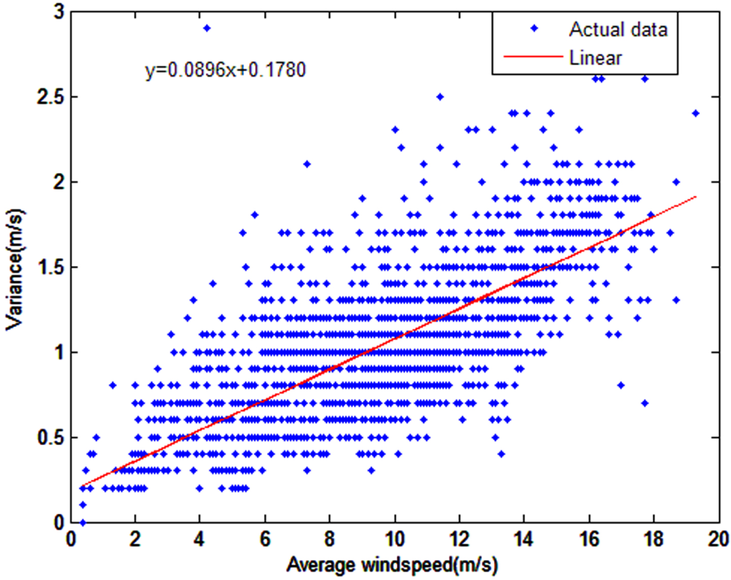
By observing the two images, it can be seen that both the average wind-speed and the wind-speed variance varies with time, and the trends of both are somewhat similar. Therefore, it is reasonable to assume that there is a connection between wind-speed variance and wind-speed. To further investigate the association between the two, the following experiments were conducted, setting the mean wind-speed as the x-axis and the wind-speed variance as the y-axis. Figure 3 illustrates the outcomes of the experiment.
Modulation effect of wind amplitude on its variance.
From Fig. 3, it can be concluded that there is a linear correlation between the two and that the wind-speed variance y varies with the mean wind-speed x. The relationship expression is: y = 0.0896x + 0.1780, which implies that the variance of the wind-speed is distinct at various times and varies with the mean wind-speed, which is a heteroskedastic task.
The noise properties of the data are assumed to satisfy a zero mean homoscedastic Gaussian distribution by a large number of contemporary regression algorithms, including conventional ELM. In contrast, statistical analysis of the acquired wind-speed dataset in the preceding section reveals that the variance varies with the mean wind-speed, which indicating that the wind operation pattern follows a Gaussian distribution of zero mean and heteroscedasticity. As a result, in this section, the optimal empirical risk loss function for the heteroscedasticity Gaussian noise signature will be derived by utilizing the Bayesian principle and maximizing a posteriori probability.
Suppose the N training data sets with heteroskedastic Gaussian noise property distribution are
If the noise in Equation (14) is Gaussian with zero mean and the homoscedastic variance σ2, the empirical risk loss function will be represented as
Based on these pioneering investigations, in order to inherit the fast advantages of ELM and obtain stable and reliable generalization performance. In this section, we combine the idea of twin hyperplanes and brings in the optimal empirical risk loss functions of homoscedastic and heteroscedastic Gaussian noise to propose two advanced models of original ELM respectively, which are called twin extreme learning machine based on heteroscedastic Gaussian noise (TELM-HGN) and twin extreme learning machine based on homoscedastic Gaussian noise (TELM-GN). The model TELM-HGN is established by solving the following optimization problems:
Where
For the purpose of resolving the optimization problem (17), the Lagrangian function is constructed as follows:
Depending on the convex optimization theory, the partial derivatives of L (β1, ξ
i
, α
i
) with respect to the parameter β1, ξ
i
, α
i
are obtained by minimizing L (β1, ξ
i
, α
i
), respectively, and the expressions are available as follows:
The optimal solution in accordance with the KKT condition can be derived as shown below:
Therefore, the lower bound nonlinear regression function is calculated as follows:
Similarly, the presentation of the Lagrangian function in (18) leads to the following expression:
Separately, it is possible to work out the partial derivatives of
Then the upper bound nonlinear function can be expressively presented as:
Each one determines the ɛ-insensitive down-bound or up-bound regressor. Hence, TELM is constructed as:
That is, when the formula (14) satisfies Gaussian noise of zero mean homovariance, TELM-HGN evolves into twin extreme learning machine based on homovariance Gaussian noise model (TELM-GN), which is also termed as twin extreme learning machine (TELM). Therefore, the model TELM-GN can be expressed in the following form:
For the solution of the optimization problem (29), the Lagrangian function is constructed as:
Derivation of the Lagrangian function
According to the KKT condition, the optimal solution can be derived as shown below:
Correspondingly, β2 can be calculated as:
Once Equations (36) are solved, two functions f1 (x) and f2 (x) are obtained, respectively, as:
According to Equations (38), the decision function of TELM*GN is expressed in the following:
The algorithm design of TELM-HGN is as follows:
Once f1 (x) and f2 (x) are obtained, respectively. The regression function of TELM-HGN is shown as follows:
Experiments and discussion
In this section, in order to adequately validate the aforementioned regression algorithm in terms of correctness and feasibility, it is evaluated against several recently published algorithms including ELM, regularized ELM (RELM), robust ELM model with truncated 2-norm loss function (RTTELM) on both public and real wind-speed datasets. All experiments were carried out on a personal notebook with Inter Core i5-8700, 4GB memory, and windows 7 operation system in python 3.7 environment such that the same platform is provided for simulations. As for activation function, the commonly used Sigmoid is chosen.
In addition, parameter selection is one of the key issues affecting model evaluation, such as the regularization coefficient and the number of hidden layer nodes have a large impact on the generalization performance of the model. There have been many algorithms [39, 40] for selecting the optimal parameters, including particle swarm optimization algorithm [41], grid search algorithm [42], gray wolf optimization algorithm [43], etc. In this paper, the more popular and general grid search method is used to optimally select the parameters of the above models, which locate the optimal solution by traversing the specified parameters in the parameter space. In an attempt to reduce the computational burden of model selection for TELM-HGN and TELM-GN, C1 = C2 and ɛ1 = ɛ2 are set in our experiments. The regularization parameters involved in these algorithms are also selected from the values of [1,1000]. Meanwhile, to evaluate the performance of the aforementioned algorithms, the following five commonly used evaluation criterions are imported before presenting the experimental results, namely, mean absolute error (MAE), mean square error (MSE), sum of error squares (SSE), total sum of squares (SST), and sum of squares of regression (SSR) to compare the learning performance of different models. Table 1 presents the predictions and definitions of each evaluation metrics.
Indicator prediction and definition
Indicator prediction and definition
Without loss of generality, assume that the mean value of the test sample is
In this section, in order to further verify the effectiveness of the model, we apply the proposed model to UCI data sets, including Boston house price data set and stock data set, Boston house prices are some data points of Boston houses (http://archive.ics.uci.edu/ml/index.php), which contain relatively few data points, only 506, and each sample has 13 characteristics to determine the trend of house prices, such as per capita crime rate, average number of rooms per house, highway accessibility, etc. The stock data set contains the historical stock data. Each sample contains nine characteristics, including the stock price at the opening of the market, the highest price of the day, the lowest price of the day, and so on. 50% of each data set is extracted as training set and test set for experimental analysis. Figure 4 shows the prediction results of the five models on stocks, and Table 2 lists the prediction errors of the five models on stocks. Figure 5 shows the prediction results of the five models on Boston house prices, and Table 3 lists the prediction errors of the five models on Boston house prices.
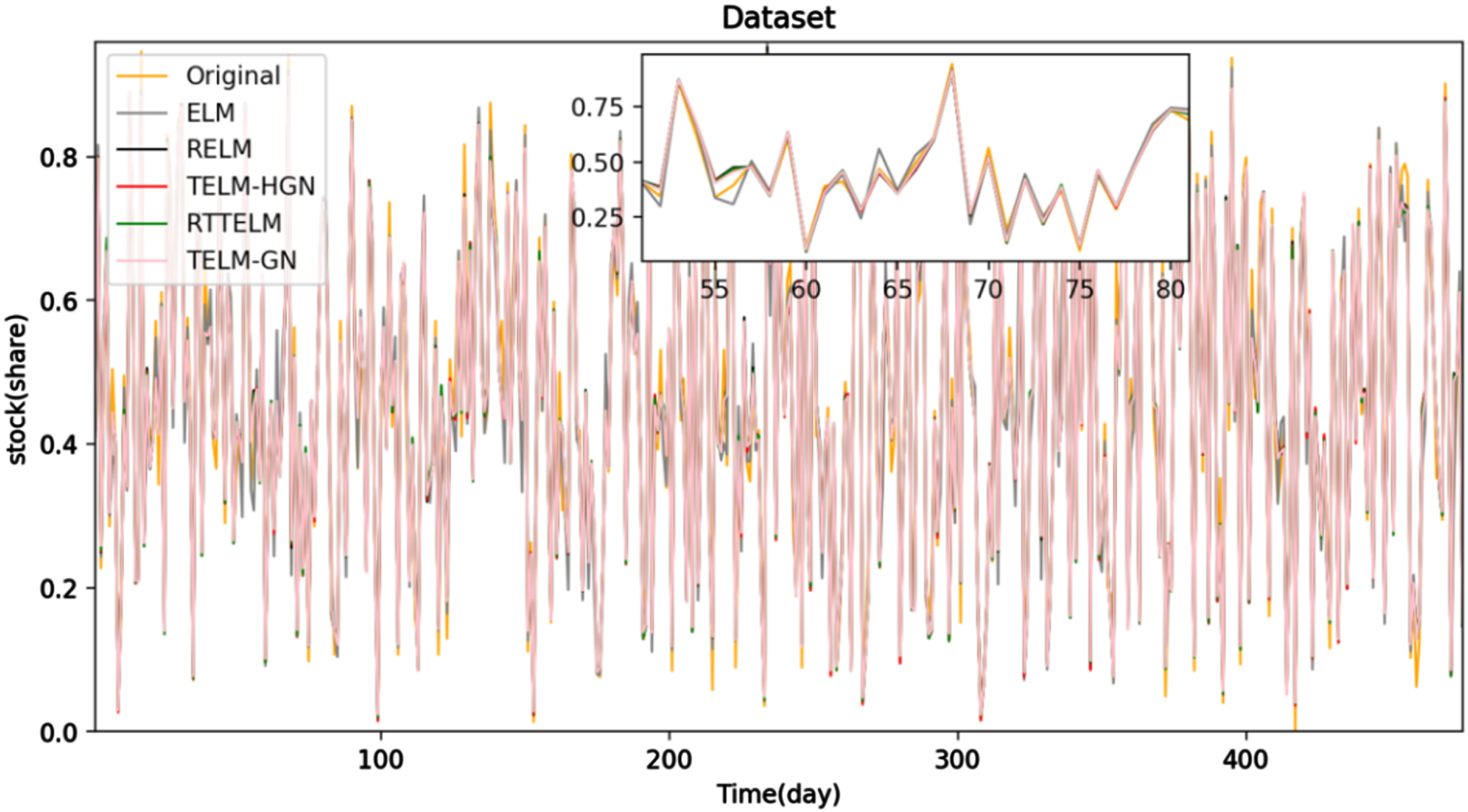
The prediction results of the five models on stocks.
The prediction errors of five models on stocks
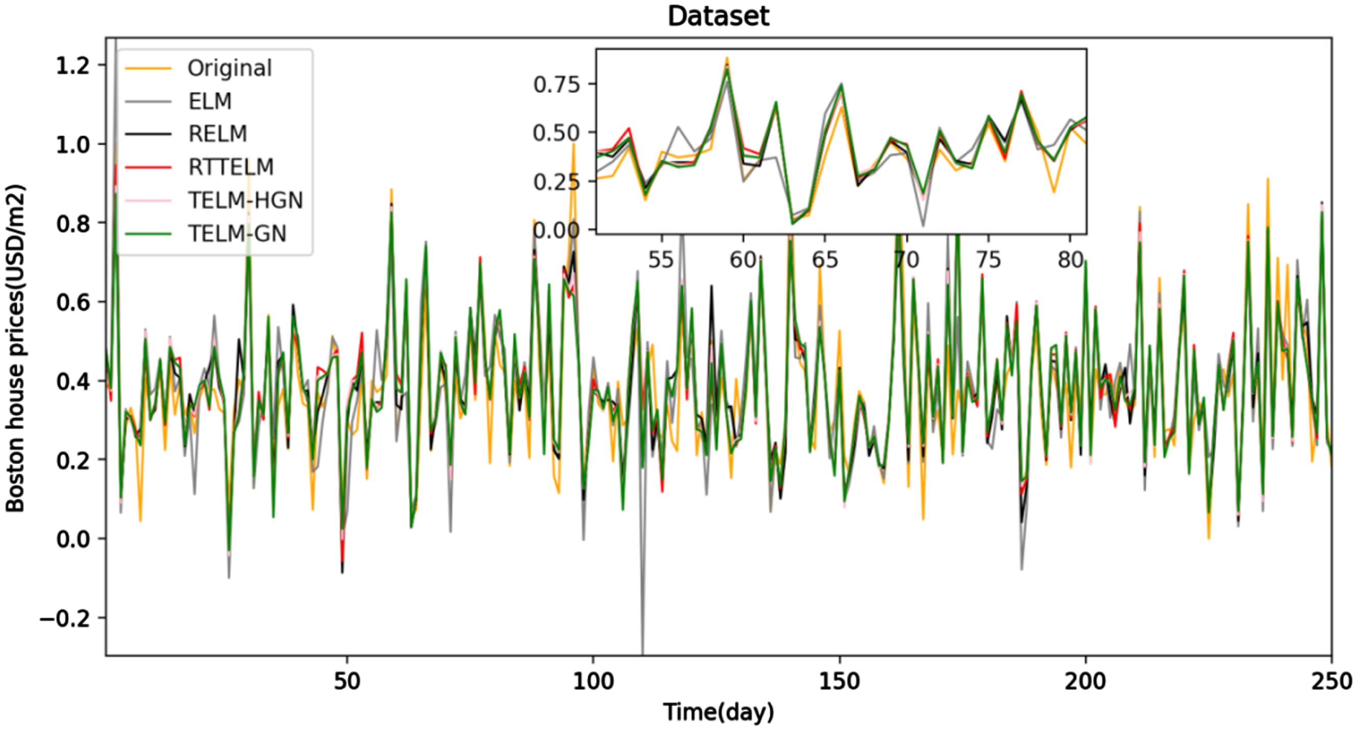
The prediction results of the five models on Boston house prices.
The prediction errors of five models on Boston house prices
From Tables 2 3, among all the algorithms, the ELM with twin spirits improves the learning effect and has the smallest evaluation standard, which is also the motivation to develop the algorithm in this paper. Specially, the proposed model derives the smallest SSE and SSE/SST, and the largest SSR/SST among these three algorithms, which indicates the statistical information in the training datasets is well presented by the proposed model with fairly small regression errors. That is to say, the presented model not only obtain more accurate prediction but also owns good generalization performance.
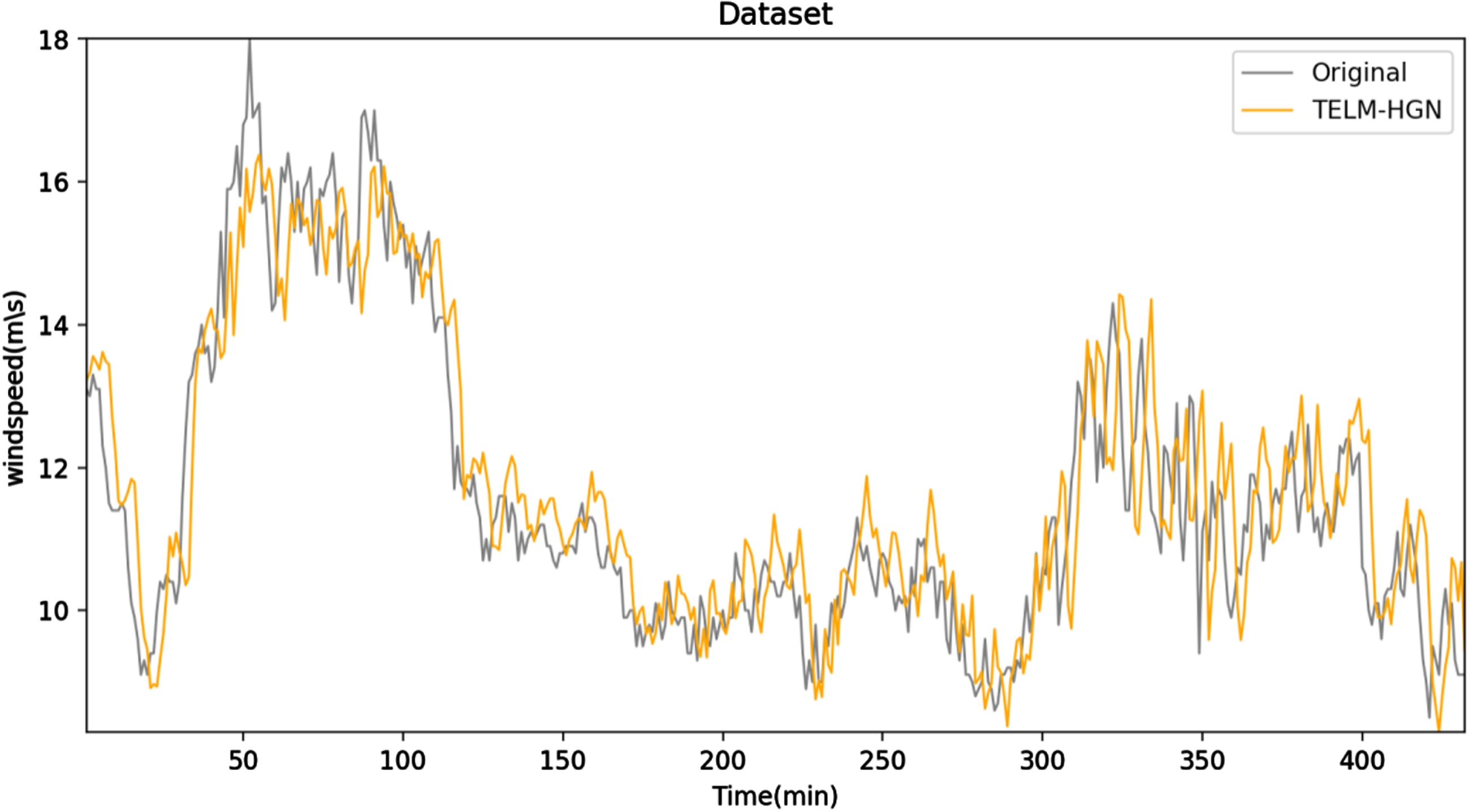
In the above subsection, TELM-HGN has demonstrated its advantages on public data sets. To further proof the benefits of the model in practical applications, one-year wind-speed data of Heilongjiang province was gathered, which yields 62,466 samples with four attributes: mean, variance, minimum, and maximum. In this experiment, 432 training samples and 432 test samples are selected for analysis, respectively. The wind-speed forecasting model is constructed as follows: the input vector

Prediction of five models on wind-speed after 10 minutes.
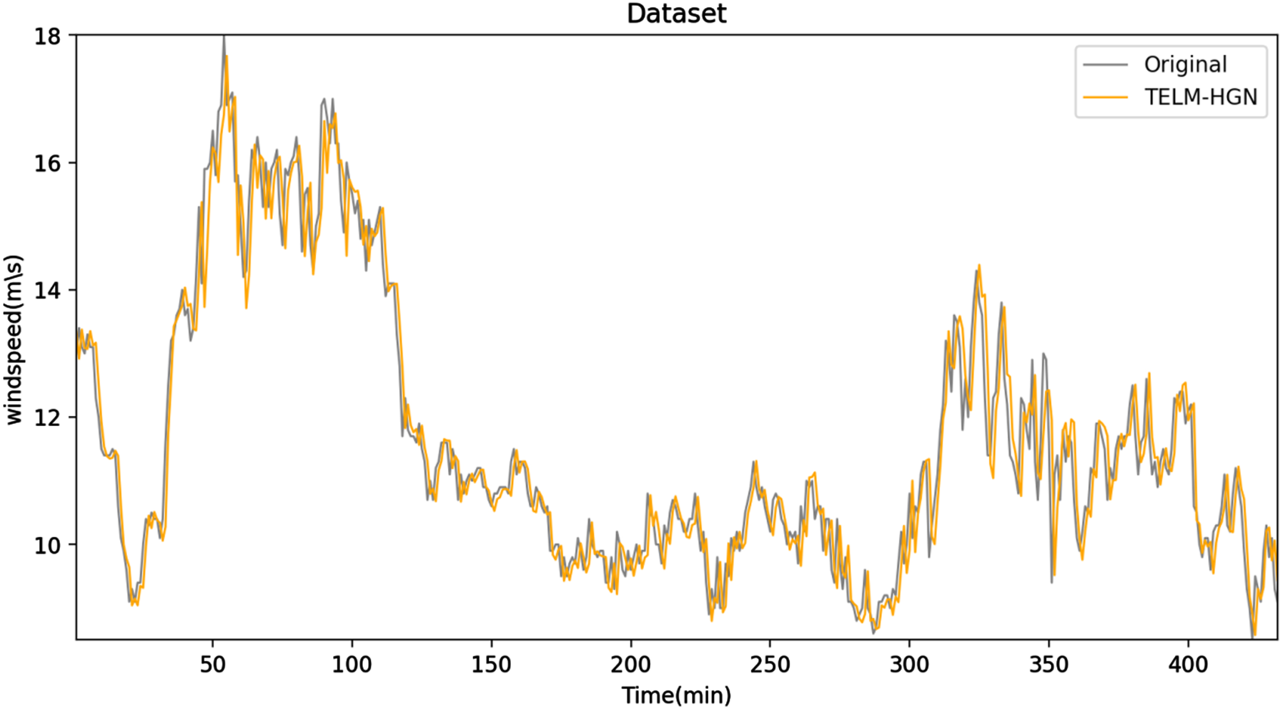
Prediction of wind-speed after 10 minutes by the proposed model.

Prediction of five models on wind-speed after 30 minutes.
Prediction of wind-speed after 30 minutes by the proposed model.
Result comparisons of five models on wind-speed after 10 min
Result comparisons of five models on wind-speed after 30 min
Tables 4 5 demonstrate that the proposed models have distinct advantages over the other comparability models, particularly in the wind-speed forecasting error statistics after 10 minutes, where the proposed model achieves smaller MAE, SSE, and SSE/SST. Furthermore, the prediction accuracy of the proposed model in terms of MSE is always the strongest. However, the performance of the TELM-GN model is improved to some extent due to the addition of twin structure, its prediction is not the best because the noise model satisfies the heteroskedastic regression task in wind-speed forecasting.
Also, as shown in Figs. 6 8, the regression curves obtained by these algorithms all deviate from the original equation to varying degrees, whereas the regression curve obtained by the proposed model is always the closest to the original system, indicating that the proposed model has a highest accuracy effect than several other models. As a result, the proposed models can be deemed an effective approach for predicting actual wind-speed.
ELM has the advantage of being efficient and fast, which has brought about a further breakthrough in the research of feedforward neural networks. However, there are some drawbacks of the ELM, such as being sensitive to noise and outliers, being susceptible to overfitting and resulting in degraded generalization performance, and being of poor stability. From a variety of perspectives, it is not considered as the most adequate model and there is much room for improvements.
This section summarizes our main work: (1) we discover that the wind operation law meets a Gaussian distribution with zero mean heteroscedasticity by investigating the properties of noise models in real wind-speed forecasting; (2) The optimal empirical risk loss function of heteroscedasticity noise characteristics is derived by using Bayes principle and maximizing posterior probability method. (3) The regression models of twin extreme learning machine based on Gaussian heteroscedasticity noise (TELM-HGN) and twin extreme learning machine based on homoscedastic Gaussian noise (TELM-GN) are established respectively; (4) Using the Lagrange function and we obtained the dual problem of TELM-HGN and TELM-GN according to KKT conditions; (5) Solving the TELM-HGN by the ALM method, which guaranteed the effectiveness and stability of the algorithm; Experiments on stock, Boston home price, and wind-speed data sets validate the validity and accuracy of the provided model by comparing it to other several models recently released algorithms. Besides, TELM-HGN not only maintains the advantages of ELM in simple parameter setting and capability of rapid convergence, but also makes up for the disadvantages of being sensitive to noise and outliers and poor generalization performance. Because of its fast throughput and strong generalization performance, it is particularly suited for large-scale data processing.
However, this work solely addresses the issue of heteroskedastic Gaussian in regression models. The real distribution of noise is complex and changeable in more practical situations. Considering the limited approximation ability of heteroscedasticity noise to simulate complex noise, the authors will investigate utilizing alternative mixed distributions to model noise distributions in real problems. In addition, we can also develop problems similar to classification learning. In other words, in the future we will study the classification problem of mixed noise characteristics.
Author Contributions
S.G. Zhang and D. Guo drafted the manuscript, conceived the algorithm and designed the experiments, D. Guo implemented the experiments; T. Zhou analyzed the results. All authors read and revised the manuscript.
Funding
This work was supported by the Natural Science Foundation of Shandong Province (ZR2022MF242); Key research and development plan of Shandong Province (2019GGX101056).
Conflicts of interest
The authors declare conflict of interest.