A combined model based on seasonal autoregressive integrated moving average and modified particle swarm optimization algorithm for electrical load forecasting

Abstract

Electric load prediction is an important decision tool in area of electricity economy. Recently researchers have presented innovative models to improve the forecasting accuracy of short-term electricity series, which is valuable in allowing both consumers and electric power sector to make effective planning. This study proposed novel combing optimization model to improve the precision of electric load forecasting and called SSPM. First, taken the advantage of linear prediction for the seasonal autoregressive integrated moving average (SARIMA) model and non-linear prediction for the support vector machines (SVM) model to combine a new model. Next, the produce results by SARIMA model is regarded as linear component and used SVM model for correcting the residual from SARIMA as non-linear component of forecasting results. Third, in order to show the dynamic relationship of linear and non-linear components, the weight variable of α₁ and α₂ are proposed that optimized by particle swarm optimization (PSO) algorithm with lower error of fitness function, the combining model is applied in the daily electric load data at New South Wales (NSW) in Australia. The experimental results indicate that the proposed optimization model obtains better performance of precise and stability than models of SARIMA and SVM respectively, outperform than conventional artificial neural network (ANN). Although the novel model is applied to electric load forecasting in this paper, it has more scopes for application in a number of areas to gain improvement of forecast accuracy in complex time series.

Keywords

Support vector machines seasonal autoregressive integrated moving average combining optimization model electric load forecasting particle swarm optimization algorithm

1 Introduction

Electricity is a special energy source that has particular attribute which cannot be stored and transported by vehicle. Therefore, effective load demand decisions should be made correctly and timely, it is important to manage the process of electrical production, distribution and consumption. Many researchers have investigated electricity prediction in current decision, but how to forecast power load with better accuracy and effectively organize the transportation sector, electricity generation sector and electricity market are still challenging tasks [1]. Because inaccuracy and uncertain prediction can waster for energy distribution and industrial production, that lead to the risk of management and the increase of the operating cost, which caused a wrong strategy in the generation of the power sector. Moreover, the accurate prediction of the power data is a complex process that including climate factor and social environment. Climate changes include season changes and temperature, among other concerns, social environment changes involve holidays, local laws, competition of Market [2]. Furthermore, many random and uncertain factors could influence electricity trend, therefore, it is hard to improve the accurate forecast trend of electricity demand.

Many prediction models for electric load have been proposed by researchers over the past two decades. According to the forecasting period, the models can be classified into short-term, interim and long-term. Short term forecasting requires high forecasting accuracy with volatility and stochastic data, and this is a challenge for models. The interim and long-term forecasting have more pattern with long history dataset, it can capture the accuracy trend and interval than the short-term forecasting. The statistics methods are widely used in the stock and energy fields, and these methods are both considered the data feature and time factors, due to analysis history rule of real data at specific point in time, it can obtained trend in the time series. These methods include linear regression, logical regression and generalized linear regression. The latter two methods can be dealt with non-linear problem after conversion. Kulkarni et al. utilized Spike Response Model (SRM) for building short term electrical load predicted model applied in the Australian Energy Market Operator (AEMO) forecasting [3]. Linear regression is good at forecasting linear type dataset and the restriction of require sample have fewer noise and conform the normal distribution.

In recent literature, artificial intelligence methods are effective to deal with non-linear data and consideration more influence factors for electrical load forecasting. Ding et al. proposed a new forecasting approach for the power output of photovoltaic system based on the improved artificial neural network and similar day selection algorithm and simulation results suggested the superiority of this approach [4]. Cai et al. presented a neural network applied to the electric load forecasting based on adaptive neural network [5]. Pillai et al. investigated the feasibility of using publicly available load and weather data to generate synthetic load profiles by means of artificial neural network (ANN) [6].

However, statistics model and artificial intelligence models are applied in their own domains and none of them really fit dataset in area of electrical load. Therefore, some researchers utilize discrete probability models integrated with neural networks to produce novel hybrid models. Sperandio et al. presented new Markov Chain model based on the Self-Organizing Map (SOM) which considered climate variables of historical trend. This model was used for electricity demand prediction on very short-term horizon [7]. Kelo et al. proposed to optimize configuration of model for focused time lagged recurrent neural network. The author utilized two methods: one implemented is that the laguarre, gamma and structure of multi-channel tapped line memory; the other implemented is that the parameter-wise optimization training processed [8]. Dihimi et al. proposed a novel echo state network optimized by modified shuffled frog leaping algorithm for prediction of short-term load and short-term temperature. At the previous stage, load or temperature time series were decomposed by Wavelet transform and forecasting accuracy was improved by Wavelet echo state network model [9]. The structure and parameters of model influence the forecasting results, and tune off still lacks on theoretical basis.

Meta heuristics can effectively optimize parameters of conventional model and improve precision for prediction. Li et al. proposed a combining annual power load prediction model which utilized fruit fly optimization algorithm to optimize parameter selection of generalized regression neural which is capable of more accuracy for prediction [10]. Lin et al. proposed a hybrid economic indices based on short-term load forecasting system are consideration electricity load predicted the impact of business indicators, which took part in the new model and obtained well forecasting effect [11]. Kavousi-Fard et al. proposed a new hybrid model to provide the short term electrical load prediction which utilized Modified Firefly Algorithm (MFA) to optimize parameter of Support Vector Regression (SVR) model [12]. Wang et al. applied residual modification method in SARIMA to predict electricity demand based on PSO optimal Fourier method [13]. The novel PSO–SVM model was proposed by Selakov et al. considerate the training strategies, aiming to find the similar time points in the recent historical data, are decided by the significant temperature variation in the early stage [14].

The hybrid model can utilize the advantages of each model and avoid the disadvantages; it can receive good results for prediction. However, in real world, in this section have large influence on prediction, the forecasting model with consideration of multiple factors and multiple conditions have a hot area. Hong et al. proposed model with seasonal SVR and Chaotic genetic algorithm which considered effect of cyclic changes element on electric load accuracy and obtained more precision [15] Felice et al. proposed numerical weather prediction models with potential benefit to predict electricity demand in Italy using the weather data factor [16]. Lopes et al. proposed a neural network based on the fuzzy ART architecture applied in electric load predicting problem [17]. The statistic model of SARIMA is good at forecasting the data with seasonal factor and linear trend, the intelligence method SVM is expert in processing multiple factor and non-linear trend. The combination of the two well-known models of SARIMA and SVM were a new method, which is applied in forecasting plant of a grid-connected photovoltaic and has obtained more forecasting accuracy than both of SARIMA and SVM respectively [18]. But for electricity consumption forecasting, the data involved uncertain and volatility factors, this may decrease the accuracy of prediction.

In this paper, the author proposed a novel combing model which consists of SARIMA model and SVM model optimized by PSO algorithm to forecast electricity consumption, this model marked SSPM. At first, the model SARIMA is used to forecast the dataset and the forecasting result as linear component for final model. The six type SARIMA models with different parameters are proposed and marked case1 to case6. The predict results of these six cases were tested by statistical analysis and selected lowest error of case as a best model. Next, the forecasting results of SVM model which set residual from the SARIMA model of first step as input data, it regard as non-linear component for final model. Third, two weights variable are represented in the dynamic relationship between linear and non-linear components with optimization by PSO algorithm. It is calculated best weight variable that combine linear and non-linear components of the above discussion, product forecasting resulting with minimum errors. Finally, the linear and non-linear components by final model are represented linear regression expression with optimization weight variable, and final forecasts are produced.

1.1 Our contributions

The electric load is a complexity process and influenced by many factors such as holiday, climate, economy, and so on. It is challenging for the improvement of forecasting precision. Electric load dataset is of special characteristics involved linear, nonlinear and both together. Linear forecasting model is particularly useful for handling the dataset which hypothesize that the unknown parameters of the model to expect relation and proportion of dataset. Nonlinear forecasting model is applied in collection with strong randomness and irregular volatility of random error. However, pure linear or pure nonlinear models rarely exist in reality, the two components are often mixed together and become major component alternately in time series. In order to precisely depict the real situation of the above discussion, in this study, the effective novel model was proposed and marked SSPM to improve forecasting accuracy in electricity load dataset in NSW. In this way, the accuracy of electric demand forecasting is improved significantly.

The remainder of this paper is organized as follows. Section 2 illustrates the innovation and the major idea. Section 3 illustrates the SARIMA model and SVM technique respectively, and the proposed combining model is described in details. Section 4 shows and discusses the results of numerical experiments, including the introduction of the criteria and the performance of the model. Finally, Section 5 deals with the conclusions and future research.

2 Methodology

This section will conduct a literature review including the description of SARIMA model, SVM model and a proposed combining model.

2.1 Seasonal autoregressive integrated moving average models (SARIMA)

Auto-Regressive Integrated Moving Average (ARIMA) is a statistics model proposed by Box and Jenkins in 1976 [19]. Specially, SARIMA model is extended from ARIMA model and considers seasonal factors, which is more suitable for time-series analysis than traditional ARIMA.

Time series {x_t|t = 1, 2, …, n} is created by a SARIMA (p, d, q) (P, D, Q) model if: $Φ_{p} (L) A_{P} (L^{s}) (Δ^{d} Δ_{s}^{D} y_{t}) = Θ_{q} (L) B_{Q} (L^{s}) v_{t}$ (1)

In which P and Q show seasonal regression; p and q demonstrate no seasonal auto-regression; d and D show separately no seasonal difference and seasonal difference, s is the period length of season. The above equation is named seasonal time series model or product seasonal model.

φ (L) =1 - φ₁L - φ₂L² - ⋯ - φ_pL^p, is the periodical operator of autoregressive (AR) of index p.

Φ (L^s) =1 - Φ₁L^s - Φ₂L^2s - ⋯ - Φ_PL^Ps, is the periodical operator of seasonal autoregressive (SAR) of index P.

θ (L) =1 - θ₁L - θ₂L² - ⋯ - θ_pL^p, is the periodical operator of moving average (MA) of index q.

Θ (L) =1 - Θ₁L^s - Θ₂L^2s - ⋯ - Θ_spL^sp, is periodical operator of seasonal moving average (SMA) of index Q.

In the equation, d and D are special presented numbers of regular differences and seasonal differences. ν_t is a white noise signal that is the estimated residual by time t (i.i.d) as a normal random variable with an average value equal to zero and a variance sigma $σ_{ɛ}^{2}$ [23, 24]. To establish the SARIMA model, the following four steps are considered:

Step 1: Confirm variable differences d and D, and original sequence conversion to stationary sequence by regular difference and seasonal difference. Order new sequence $x_{t} = Δ^{d} Δ_{s}^{D} y_{t}$ .

Step 2: Confirm p, q, P, Q values by parameters estimate of SARIMA.

Step 3: Build suitable model with Equation (1) and test the accuracy of the chosen model.

Step 4: Utilize the chosen model to predict the future data of the sequence, and delivered in a confidence interval.

From the above introduction, the conventional SARIMA model is good at analyzing data with seasonal factors and upward trend in time series. The parameter of SARIMA is adjustable for available experimental data and texted with statistical techniques.

2.2 Support Vector Machine (SVM)

Vapnik et al. firstly proposed SVM conception as a tool of statistics learning [20]. The model is often applied in range of classification and regression problems and has obtained a good effect. The algorithm solves complex surfaces in spatial of high dimension with support vector which represents vector of sample.

The principal advantage of SVM is made of empirical risk for minimization and validation with possibility of determining an acceptable error. The SVR can solve problems of regression based on principle of SVM. On the basis of literature survey, some researcher begins to study how to use SVR model for the prediction of time series and function. The principle of SVM is as follows.

Suppose the training dataset {x_i, y_i}, (i = 1, 2, …, n) where x_i is the input vector of dimension n and x_i ∈ Rⁿ, y_i is output value of x_i, name labels of output y_i ∈ R. Given a positive real number e, a function f (x_i) does not deviate from y_i by more than e, the SVM approximates is defined as follows: $f (x) = 〈 w, φ (x) 〉 + b,$ (2)

The minimization standard weight is given as follows: $min \frac{1}{2} {∥ w ∥}^{2}$ (3) $s . t | y_{t} - 〈 w, φ (x_{i}) 〉 - b | \leq ɛ, i = 1, \dots N$

In which φ (x) is feature function and maps a nonlinear function from input vector x, w is weights of vector, and b is a constant. In order to improve recognition of excessive noise or outliers, the slack variables $ξ_{i}, ξ_{i}^{*}$ are introduced to the new formula: $min \frac{1}{2} {∥ w ∥}^{2} + C \sum_{i = 1}^{N} (ξ_{i} + ξ_{i}^{*})$ (4) with the following constraints: $\begin{matrix} y_{i} - 〈 w, φ (x_{i}) 〉 - b \leq ɛ + ξ_{i} \\ 〈 w, φ (x_{i}) 〉 + b - y_{i} \leq ɛ + ξ_{i}^{*} \\ ξ_{i}, ξ_{i}^{*} \geq 0, i = 1, \dots, N \end{matrix}$ in which ξ_i and $ξ_{i}^{*}$ are present absolutely error scope whose values are positive or negative. Constant C named hyper-parameter is used to adjust the flatness of the function f and the amount of authorized error. Error function |ξ|_ɛ is used to validate formulation data range:

$\begin{matrix} {| y - f (x) |}_{ɛ} \\ = {\begin{matrix} | y - f (x) | - ɛ, & for | y - f (x) | > ɛ \\ 0, & otherwise \end{matrix} \end{matrix}$ (5)

In order to facilitate the calculation process, the Equation (4) is translated by Lagrange formulation as follow:

$\begin{matrix} L & = & - \frac{1}{2} \sum_{i, j = 1}^{N} (α_{i} - α_{i}^{*}) (α_{j} - α_{j}^{*}) k (x_{i}, x_{j}) \\ - ɛ \sum_{i = 1}^{N} (α_{i} + α_{i}^{*}) + \sum_{i = 1}^{N} yi (α_{i} - α_{i}^{*}) \end{matrix}$ (6)

The constants α_i and $α_{i}^{*}$ must be positive and are named Lagrange multipliers with the condition of $\sum_{i = 1}^{N} (α_{i} - α_{i}^{*}) = 0$ $α_{i}, α_{i}^{*} \in [0, C]$ . The formula of the model’s weight is described as follow: $w = \sum_{i = 1}^{n} (α_{i} - α_{i}^{*}) φ (x_{i})$ (7)

Thus, the model can be described through the operation: $f (x) = \sum_{i = 1}^{N} y_{i} (α_{i} - α_{i}^{*}) k (x_{i}, x) + b$ (8)

The function k is called kernel function and it maps nonlinear dataset into high dimension space with conditions of Karush-Kuhn-Tucker (KKT). Thereby, the Equation (8) generates linear classification from nonlinear dataset [21].

2.3 Combining model

The principal aim is to develop the forecasting performance of the combining model with respect to the electricity load in short-term time series. Literature [22] proposed forecasting models which process forecasting results of linear and non-linear components respectively to improve forecasting accuracy. However, the variables of the two components are only simple combination to produce forecasting results and do not show the dynamic relationship of linear and non-linear, because in the real dataset, the main degree of linear and non-linear are dynamic change in the time series, it is important to differentiate relationship of two components, and it has a great influence on the final forecasting precision. From the above, the weight variables of α₁ and α₂ are proposed to reflect the relationship between of linear and non-linear components, the calculation as follow: ${\hat{y}}_{t} = α_{1} {\hat{L}}_{t} + α_{2} {\hat{N}}_{t}, t = 1, 2 \dots n α_{1} + α_{2} = 1$ (9) in which variables of α₁ and α₂ are weight factors of ${\hat{L}}_{t}$ and ${\hat{N}}_{t}$ components. In order to indicate the relation of the two components and improve accuracy of prediction, the two variables α₁ and α₂ are optimized by PSO algorithm with capability of obtaining global optimal solution [23]. Then, the SSPM is applied for forecasting with optimal variable weights and the performance of the novel model is tested by statistics technique.

Algorithm 1. SSPM
Input:
X = (x_t1, x_t2 … x_ti) , t = 1, 2 ⋯ k, i = 1, 2 ⋯ n— a sequence of time series data.
Y = (y_t1, y_t2 ⋯ y_ti) , t = 1, 2 ⋯ k, i = 1, 2 ⋯ n— the value of correspond to a sequence of time series data.
Output:
${\hat{y}}_{t}$ — final forecasting value for setting cycle range.
Parameters:
q — the number of non-seasonal moving average terms.
p — the number of non – seasonal autoregressive terms.
d — the number of regular differences.
P — the number of seasonal autoregressive terms.
Q — the number of seasonal moving average terms.
D — the number of seasonal differences.
S — the seasonality of the model.
popsize — the population size of the solution space.
iter_num— the max time of particle iteration.
α₁, α₂ — the weight values of linear and non-linear components.
1:/* Confirm variable differences d and D, and original sequence conversion to stationary sequence by regular difference and seasonal difference. */
2: FOR EACHp, q, P, QDO
Confirm p, q, P, Q values by parameters estimate of SARIMA. Illustration is in Section 2 of SARIMA.
3: Utilize statistics test ACF and PCF to determined feasibility of model.
4: The forecasting value by generated SARIMA is regard as linear component for final model and set ${\hat{L}}_{t}$
5: END FOR
/The residual by produced SARIMA as the input data series for SVM model/
6: SET the residual is divided into training data and testing data DO
7: The forecasting value of SVM is regarded as non-linear component for final model and set ${\hat{N}}_{t}$ .
8: Initialization the value of α₁ and α₂ for fitness function.
Illustration in Equation 9.
9: FOR EACH i > 1 ANDi < = popsize DO
10: α₁ = ARRAY (1, rang); α₂ = ARRAY (1, rang);
11: END FOR
12: P = {α₁, α₂}; iter = 1;
13: WHILE (iter < = iter_num) DO
14:/* Find the global value of special range*/
15: FOR EACHpiDO
16: Calculation the fitness (pi) value based on function $f_{optimze} = \sum_{t = 1}^{n} \| y_{t} - α_{1} \times {\hat{L}}_{t} - α_{2} \times {\hat{N}}_{t} \|$
17: IF (pBest_i > fitness (pi)) THEN
18: pBest_i = fitness (p_i);
19: END IF
20: END FOR
21: FOR EACHiinPDO
22: Update gBest and record the best particle;
23: Update value
v_i+1 = w × v_i + c₁ × rnd × (pBest_i - p_i) + c₂ × rnd × (gBest - p_i)
24: p_i+1 = p_i + v_i;
25: END FOR
26: iter = iter+1;
27: END WHILE
28: RETURN α_1best and α_2best
29: Calculation value ${\hat{y}}_{t} = α_{1} {\hat{L}}_{t} + α_{2} {\hat{N}}_{t},$

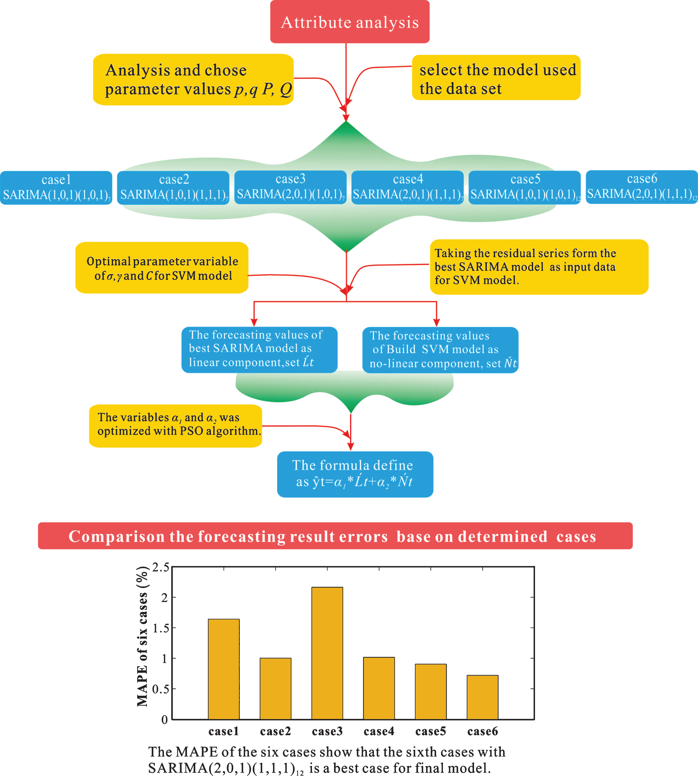
The objective function of optimization for PSO is defined as follow: $f_{optimze} = \sum_{t = 1}^{n} | y_{t} - α_{1} \times {\hat{L}}_{t} - α_{2} \times {\hat{N}}_{t} |$ (10) in which the variables α₁ and α₂ are parameters of optimization in the range from 0 to 1 by means of PSO method, ${\hat{L}}_{t}$ and ${\hat{N}}_{t}$ are linear and nonlinear components for SSPM and y_t is an actual data. In order to obtain minimum values, the optimization function is defined as the non-negative function and the population size of the optimization process of PSO algorithm is 50, the range of popular size will be discussed in Section 4.1. The SSPM algorithm and flow chart are show in Algorithm 1 and Fig. 1, respectively.

Fig.1

The flow chart of proposed model combined SARIMA and SVM method.

In this section, first, the dataset was detection by SARIMA model. Weather detection SARIMA model will validate the model through statistical techniques. The seasonal factors have been considered in determining model.

The Auto Correlation Function (ACF) and Partial Correlation Function (PCF) method have been used to test the feasibility of the SARIMA model. Second, the six cases were proposed based on different parameter of SARIMA model, the best case selected with performance analysis criteria and regard as best SARIMA model. By the adoption of the best SARIMA model, the forecasting results are regarded as linear component for SSPM and the residual has been regarded as the input data for SVM model. Finally, two weight variables are optimized by PSO algorithm and the final model is obtained.

By the adoption of the PSO algorithm, the global optimal solution is obtained, and then forecast the value with α_1best and α_2best to calculate the linear and non-linear component.

3 Experiment and discussion

The proposed model utilizes the advantages of SARIMA for linear component and SVM for nonlinear component. So in the first step, the input data of regularization base on seasonal ARIMA model and linear components have been obtained with marked ${\hat{L}}_{t}$ . The second step, the residual generated by SARIMA model is taken as input data of SVM model with strongly capable of nonlinear processing. In this way, the nonlinear component is generated by SVM and labeled ${\hat{N}}_{t}$ . Finally, two weights variable of a₁ and a₂ are optimized by PSO algorithm, by the adoption of linear and non-linear components with best weighs variable, the final forecast results by Equation 9 is calculated.

3.1 Electric load dataset

The experimental dataset was conducted by adopting every 30 min data of NSW in Australia from AEMO, it is the largest energy market in Australia, and then precision electricity load forecasting is important for operating and planning of the power system. Every day has 48 points value, the day dataset is generated for raw data with average of the 48 data points as data points. From the above, the data collection of electric demand from January 2009 to December 2011 (3 years), and averaged 48 time points as one day data. Figure 2 illustrates the electric load data of NSW with seasonal and random factors in the time series. In order to pass statistical testing, an auto correlation analysis has been applied to find a seasonal pattern. The auto correlation of original data was shown in Fig. 2(b), which has obvious seasonality pattern.

Fig.2

(a) Showing electric load dataset of three years in Australia and (b) showing auto correlation of sample.

Figure 2 shows day dataset, which were representative of electric data. Because the monthly data of January is a first time for this year, the monthly data of May is a time which alternated spring and summer, this show changed electrocution consumption in the two seasons. The monthly data September and November were shown the difficult consumption trend of autumn and winter. During the period of the observation, the time series maintain a weekly seasonality and keep 12 units in one month seasonality. In order to improve forecasting accuracy, the working day datasets are extracted, which means that datasets are a composition of observation data from Monday to Friday on a week.

In order to improve forecast precision, the original data are progressed to collect the same point in every month, and the range of day is represented λ. The set input method is show in Fig. 3. This means that if the day ith is forecast by used same day in lag λ month, Experiment show the variable of λ is 5. In the same way, the rest set are preprocessed.

Fig.3

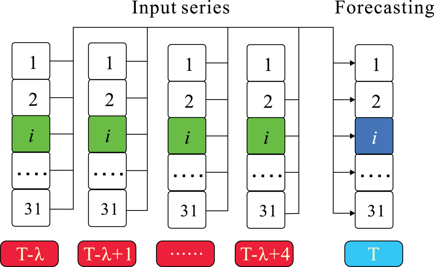
Set input series pattern.

3.2 Performance criteria

In order to obtain useful results for predictions and evaluating the performance of the proposed model, several criteria have been taken into account. The final aim is to assure the proposed optimization of the model. The generalization error of estimation has been calculated by adopting four performance indexes: the Root Mean Square Error (RMSE), the Mean Absolute Error (MAE) and the Mean Absolute Percentage Error (MAPE). Table 1 shows these performance criteria and calculation formulae separately.

Table 1
The Performance criteria and their definitions for forecasting models

Criterion Calculation

R $R = \sum_{i = 1}^{N} (O_{i} - \bar{O}) (P_{i} - \bar{P}) / \sqrt{\sum_{i = 1}^{N} (O_{i} - \bar{O})^{2} \cdot (P_{i} - \bar{P})^{2}}$

RMSE $RMSE = \sqrt{\frac{1}{N} \sum_{i = 1}^{N} (O_{i} - P_{i})^{2}}$

MAE $MAE = \frac{1}{N} \sum_{i = 1}^{N} | O_{i} - P_{i} |$

MAPE $MAPE = \frac{1}{N} \sum_{i = 1}^{N} | \frac{P_{i} - O_{i}}{O_{i}} | \times 100 %$

Criterion	Calculation
R	$R = \sum_{i = 1}^{N} (O_{i} - \bar{O}) (P_{i} - \bar{P}) / \sqrt{\sum_{i = 1}^{N} (O_{i} - \bar{O})^{2} \cdot (P_{i} - \bar{P})^{2}}$
RMSE	$RMSE = \sqrt{\frac{1}{N} \sum_{i = 1}^{N} (O_{i} - P_{i})^{2}}$
MAE	$MAE = \frac{1}{N} \sum_{i = 1}^{N} \| O_{i} - P_{i} \|$
MAPE	$MAPE = \frac{1}{N} \sum_{i = 1}^{N} \| \frac{P_{i} - O_{i}}{O_{i}} \| \times 100 %$

In Table 1, O_i is the observed value, P_i is the predicted value in time i and N is the sample number in the data series. The lower values of RMSE, MAPE and MAE show better performance.

3.3 Experimental setup

The simulate programmer compared the performance of SSPM with other models of SARIMA, SVM and other hybrid models of SARIMA combining SVM model which was marked SSM and SARIMA combining artificial neutral network (ANN) model which was marked SNNM. All the models have forecasting one month period.

At first the six cases with different parameters of SARIMA models were processed and tested by statistical technique, the best case was selected and regard as best SARIMA model in which parameter set the q = 1 and p = 2, the season variable of Q and P are 1 and 1, the diffident variable d is 0 and D is 12. SVM model parameter c and σ are equal to 1.5 and 2, the data set of preprocess were divided into train dataset and test dataset, the train to verify ratio was set 5:1, the kernel function was adopted RBF.

For the hybrid method, the other commonly models were considered, such as ARMA, hidden Markov forecasting model, classification and regression tree (CART) model, and the experiment result of these commonly models were of poor performance for this instance, so the combining model of SSM and SNNM were the only consideration in this experiment.

3.4 Experiment

The SSPM model is used to forecast electricity of one month period. At first set, the six cases were proposed from SARIMA model with diffidence parameters, these cases have marked case1 to case6. The translate cases were used to determine best parameter of SARIMA model of the experiment result. Next, the residual is generated by selecting the best case and regarded as the input dataset for SVM model, the forecasting results of SVM model as non-linear component for final model. The third step, weights variables were optimized by PSO algorithm and the final forecasting results are obtained.

The SARIMA model tested by statistical criteria of ACF and PCF was shown in Fig. 4, the six cases are executed and cases errors analysis were shown in Fig. 5, the six cases performance analysis with statistical technique were shown in Table 2.

Fig.4

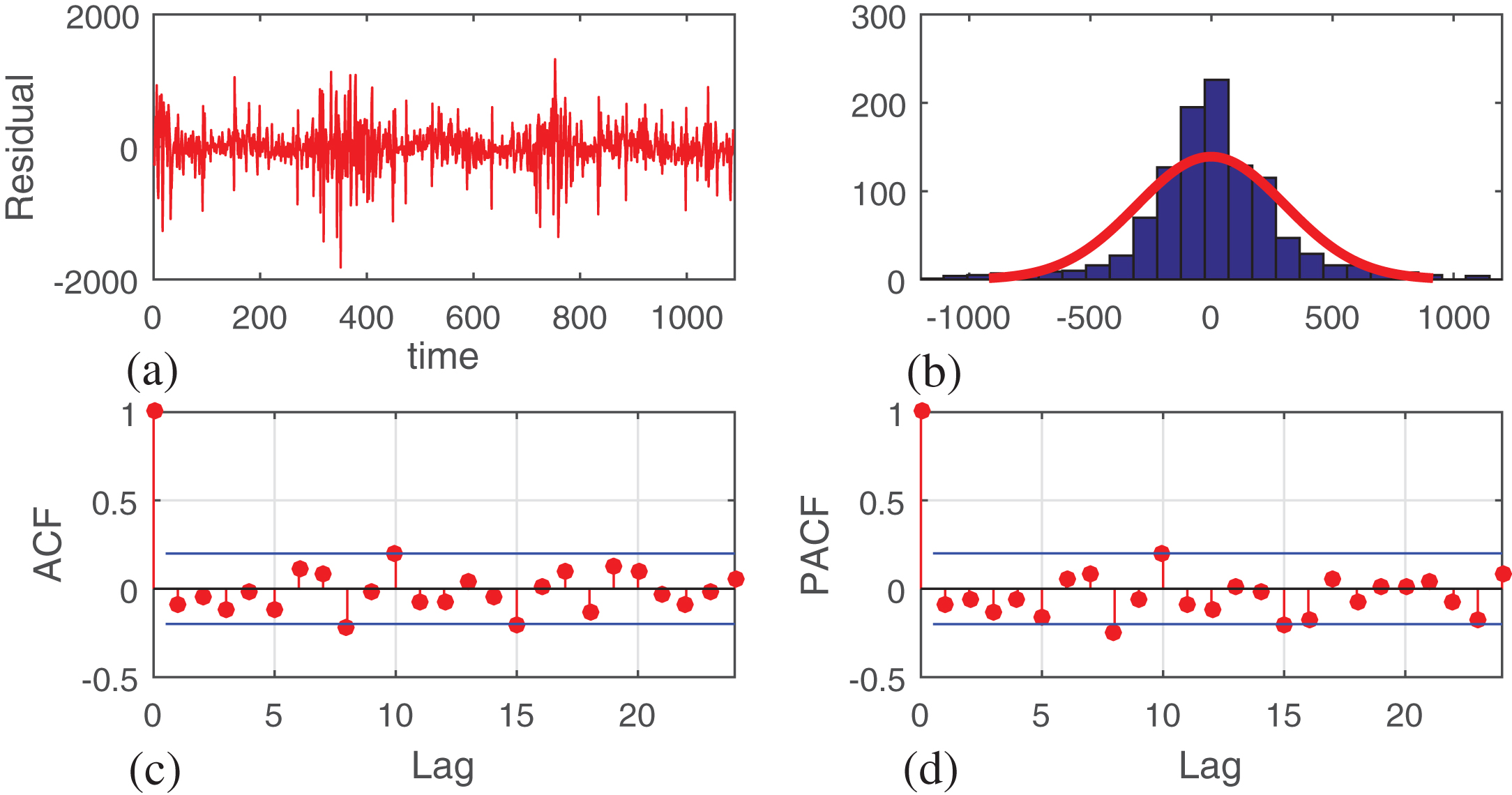
(a) The residual patterns of SAIRMA model; (b) The standard residuals histogram; (c) Sample ACF of residual; (d) Partial ACF of residual.

Fig.5

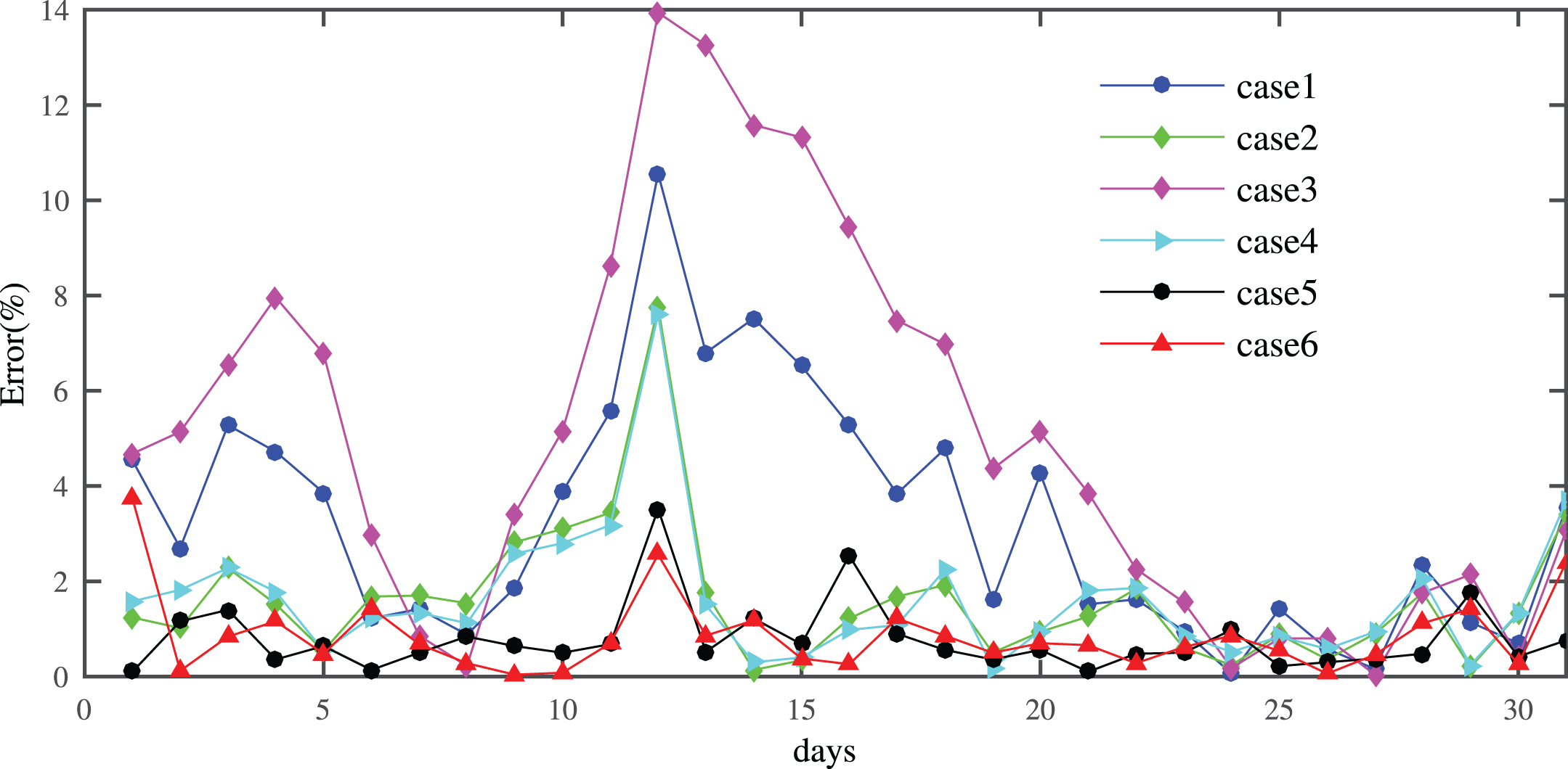
Comparison of forecasting errors for six cases on per time point with testing dataset.

Table 2

Results of the SARIMA model in the first step with best model in bold

Model (parameters)	Performance indexes
	R-squared	RMSE	MAPE(%)	MAE
Case1 (SARIMA(1,0,1)(1,0,1)₇)	0.9112	309.29	1.641	207.204
Case2 (SARIMA(1,0,1)(1,1,1)₇)	0.9112	317.403	1.002	207.696
Case3 (SARIMA(2,0,1)(1,0,1)₇)	0.8309	418.01	2.163	297.94
Case4 (SARIMA(2,0,1)(1,1,1)₇)	0.9147	306.58	1.016	206.74
Case5 (SARIMA(1,0,1)(1,0,1)₁₂)	0.9326	298.84	0.904	196.098
Case6 (SARIMA(2,0,1)(1,1,1)₁₂)	0.9357	290.87	0.720	187.820

In order to pass the statistical testing for model, an analysis method of the residuals has been implemented to ensure that the residual data satisfy a white noise process. Figure 4 (c) and (d) show no significant autocorrelation in the residual errors. It shows that the all parameter values of SARIMA models satisfy the statistical testing. The experiment results and six cases errors analysis were shown in Fig. 5.

The electricity load data was divided into two parts with train and verify ratio, which was analyzed by ACF and PCF, six cases were classified with different parameters of q, p, P, Q, d and D, thus, the six different executing result were produced. The case6 was best case which has lowest average error in six cases and does not exceed 0.75%, the case3 has maximum average error and reached 2.163%, the forecasting errors of six cases with testing dataset, were shown in Fig. 5. It shows that the case3 has larger volatility in per time point than other cases, the case5 has similar error with case6, from the plot showing, and it obviously seemed that the red color curve of case6 has always low error than other cases at per point, so the sixth case was the best model. The experiment results of six cases were shown in Table 2 with performance criteria.

Considering one-month period prediction, the chosen best case from the conversion dataset was case6 which was equal to SARIMA (2,0,1)(1,1,1)₁₂, the case6 have lowest RMSE, MAPE and MAE were 290.87, 0.720% and 187.820 respectively, this illustrated that the case6 has more fitness the actual data and the value R was 0.9357, it indicates that case6 is the best than the other five cases. The case6 has been selected as the best case, the forecasting results be taken as linear component for final model.

The forecasting results of models of SSPM, SARIMA, SNNM, SSM and SVM, and their errors were shown in Fig. 6. The performance of the five models are compared with statistical criterion, and indicated in Table 3.

Fig.6

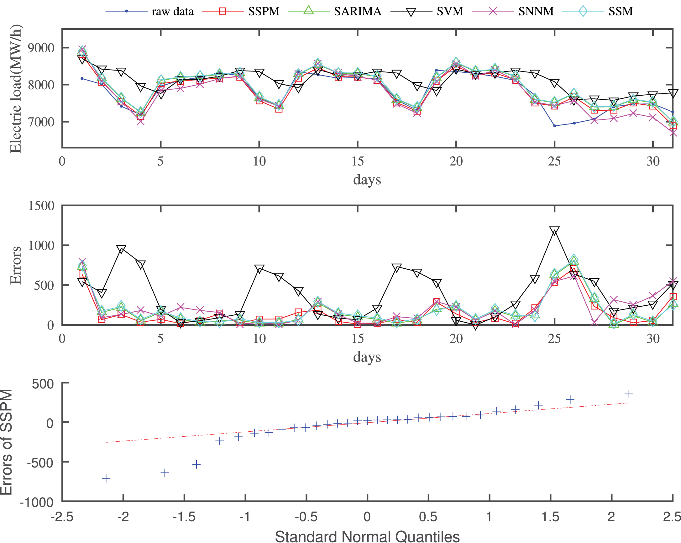
Compares the forecasting results from three models.

Table 3

Prediction errors compared of SSPM, SARIMA, SVM, SNNP and SSM models separately for one month

Site	α₁	α₂	Methods	MAPE (%)	MAE (MW/h)	RMSE (MW/h)
NSW	–	–	SVM	4.655	348.914	467.491
	–	–	SARIMA	2.348	187.82	290.87
	1.000	1.000	SNNM	2.458	188.797	271.317
	1.000	1.000	SSM	2.159	166.719	233.93
	0.901	0.098	SSPM	1.974	149.745	232.797

The five forecasting models have fitness the actual curve well and the SSPM performance outperformed than other models. The forecasting curves shows that SSPM almost coincide with raw data in overall time period. For the time zone of 23 to 26, all the models have large errors and the reason is that the electricity load is greater in the end of month than other time, such as at weekends.

The MAPE of forecasting errors for SSPM, SARIMA, SVM, SNNM and SSM were 1.974%, 2.348%, 4.655%, 2.458% and 2.159%, respectively, the max values of five models does not exceed 10%, this indicates that these models satisfy the electricity forecasting. The SSPM has lowest MAE and RMSE in five models, so the SSPM outperform than the SARIMA, SVM, SNNM and SSM. However, the values of RMSE and MAE for SSPM were close to SSM, because the parts of linear component of SSPM were made from SARIMA model and two models both used the linear component as parts of forecasting results.

The two components for SSPM were optimized by PSO algorithm, in order to represent relationship between linear and non-linear components. The argument of α₁ and α₂ dynamic weight changes by PSO algorithm are shown in Tabe.4.

From Table 4, it is obviously that the absolute errors change with parameter values of α₁ and α₂, when α₁ was close to 0.9 and α₂ is near 0.1, the absolute error decreases rapidly. In this section, the best weight value of α₁ was 0.9019, the weight value of α₂ was 0.0981 and the global best value was 4642.25 with optimization by PSO algorithm.

Table 4

The weight values of variable α₁ and α₂ with the corresponding absolute errors base on PSO algorithm

No.	α₁	α₂	Absolute error	No.	α₁	α₂	Absolute error
1	0.3012	0.6988	17714.84	26	0.2967	0.7033	12391.56
2	0.4709	0.5291	18274.41	27	0.3188	0.6812	17202.90
3	0.2305	0.7695	15944.06	28	0.4242	0.5758	16129.24
4	0.8443	0.1557	9064.37	29	0.5079	0.4921	11576.76
5	0.1948	0.8052	5310.24	30	0.0855	0.9145	13740.16
6	0.2259	0.7741	6773.60	31	0.2625	0.7375	14874.65
7	0.1707	0.8293	13626.59	32	0.8010	0.1990	17741.59
8	0.2277	0.7723	12817.41	33	0.0292	0.9708	8670.62
9	0.4357	0.5643	14452.43	34	0.9289	0.0711	9849.04
10	0.3111	0.6889	12224.56	35	0.7303	0.2697	13441.75
11	0.9234	0.0766	5171.77	36	0.4886	0.5114	19575.74
12	0.4302	0.5698	9934.06	37	0.5785	0.4215	14282.62
13	0.1848	0.8152	15603.13	38	0.2373	0.7627	10059.39
14	0.9049	0.0951	5183.24	39	0.4588	0.5412	9474.66
15	0.9797	0.0203	5180.04	40	0.9631	0.0369	7286.42
16	0.4389	0.5611	17829.36	41	0.5468	0.4532	13671.24
17	0.1111	0.8889	6749.84	42	0.9019^*	0.0981^*	4642.25 ^*
18	0.2581	0.7419	14005.04	43	0.2316	0.7684	21521.76
19	0.4087	0.5913	14036.42	44	0.4889	0.5111	10480.83
20	0.5949	0.4051	12707.76	45	0.6241	0.3759	12024.93
21	0.2622	0.7378	14907.08	46	0.6791	0.3209	16381.16
22	0.6028	0.3972	10050.45	47	0.3955	0.6045	16369.19
23	0.7112	0.2888	9650.45	48	0.3674	0.6326	14476.55
24	0.2217	0.7783	18103.97	49	0.9880	0.0120	53082.32
25	0.1174	0.8826	12236.35	50	0.0377	0.9623	13226.14

^*The best weights variable for α₁ and α₂ were bold by optimized PSO algorithm.

From the experiment results, the SSPM model is lowest in RMSE, MAPE and MAE, is 232.797, 1.974 and 149.745, respectively, the performance is better than other four models. The SVM model has maximum values of RMSE, MAPE and MAE, are 467.491, 4.655 and 348.914, respectively, this experimental results shows that the performance of SVM was impacted with large fluctuation values in the whole testing dataset. The performance of SSM is similar to SSPM, but SSM has large error at part time points of 23 to 26 days in a month, the reason is that the electricity consumption dramatically changed in time interval and the relationship of linear and non-linear components have large volatility which affected precision of final forecasting results.

4 Forecasting error analysis

4.1 Population size

The decline trend of the absolute error values by PSO algorithm was shown in Fig. 7, the error values reduce quickly and convergence with increasing iterations. With no more than 500 iterations, the best values are calculated and the relationship between two components was found out by PSO algorithm. The comparison results of three population sizes with three iterations were shown in Fig. 7(a-c).

Fig.7

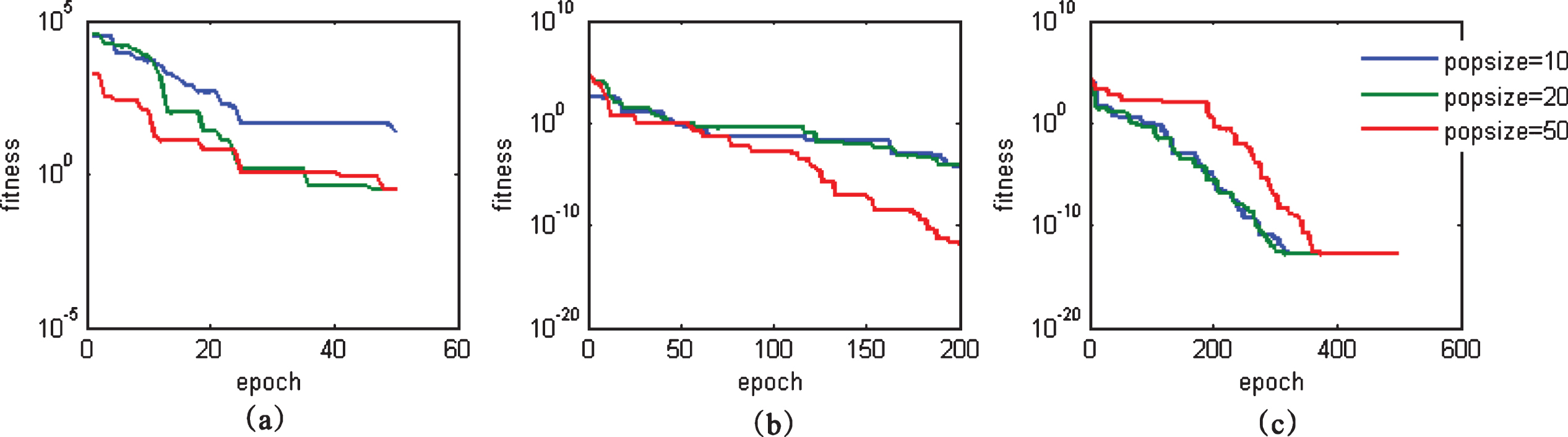
The value of absolute error for PSO algorithm which obtained weight variable α₁ and α₂.

An illustration of particle evolution with the fitness function was compared in electricity load, Fig. 7 (a-c) compare the evolutions among PSO algorithm with three epochs, Fig. 7(a) shows changes of fitness values in 10, 20 and 50 population size with 50 epochs, Similarly Fig. 7(b-c) shows that fitness changes the values in 10, 20 and 50 populations size with 200 epochs and 500 epochs, respectively. From the above, it has shown that the lager population size can make particle faster convergence for globe optimal solution. However, large population size has high runtime, the increase time complexity depends on both number of epochs and size of population. According to this experiment study, the iteration number can be set 100–200 and population size can be set 30–50. On the other hand, too large population can make particle excessive divergence, it is not convergence to globe solution in per processing and need run multiple times to find solution.

4.2 Model evaluation

The evaluation hybrid model performance methods of Dynamic Time Warping (DTW) and the Two-Order Forecasting Validity (TOFV) were used to analyze the performance of the each model in this paper [24]. DTW method measures the similarity between two temporal sequences which may vary in speed. DTW has often been applied in temporal sequence of video and graphics data. The method of two-order forecasting validity uses prediction accuracy and standard deviation of prediction to evaluate the performance of combining forecasting models. The two methods are used to evaluate the prediction performance of five methods for forecasting electric load in NSW of Australian. The comparison of forecasting results and experimental analysis in details are shown in Table 5. The lower values of DTW and higher values of TOFV show better performance of models.

Table 5
Evaluation the prediction performance of five forecasting engines based on evaluation models of DTW and TOFV

Data Set Methods SVM SARIMA SNNM SSM SSPM

NSW DTW 431.4365 192.4535 173.993 203.4061 161.096

TOFV 0.9741 0.9832 0.9815 0.9807 0.9854

Data Set	Methods	SVM	SARIMA	SNNM	SSM	SSPM
NSW	DTW	431.4365	192.4535	173.993	203.4061	161.096
	TOFV	0.9741	0.9832	0.9815	0.9807	0.9854

The forecasting error analysis illustrated that the SSPM model has better performance than other model, it indicated that the SSPM have lower error throughout the whole dataset, but at some time point large errors like both ends points of the testing dataset will appear, the reason was that the information is lack of the previous day’s history and unable estimated the beginning trend for dataset. However, the forecasting accuracy will make balance between consumption and supply of electricity, and rational utilization power resources. A low forecasting error will lead to precise reserve estimation effectively and reduce risk of administration for power grid and operation costs. The forecasting error increased 1%, the corresponding operating cost will increase $10 million [35]. Therefore, it is important to improve the accuracy of electricity load. In this paper, the SSPM forecasting performance exceeds the conventional models and combining model, and satisfies the forecasting electricity load.

5 Conclusion

For classical models, some models are good at dealing with linear components and other methods are good at handling nonlinear components in time series. Several researchers have found that combing approach is able to outperform either of the models used separately [2]. However, some studies pointed out that discrepancy in the research finding arising from their hypothesis.

To overcome limitations existed in the above discussed models and obtain more accurate prediction results, a novel optimization approach is proposed and marked SSPM model for electric load forecasting, which is able to do predict in time series with noisy data. The SSPM was evaluated and compared with not only SARIMA and SVM models, but also compared with other well-known combining models such as SSM and SNNM models, in the daily electric load data at NSW in Australia. The performance and capability of the models are measured and evaluated with criteria R, RMSE, MAPE and MAE. The experimental results show that the SSPM outperforms other models. Furthermore, the weights variables of α₁ and α₂ optimized by PSO algorithm in Equation 9 can finally generate more accurate prediction; it improves the forecasting accuracy of one month period. This study indicates that the SSPM is an inerrable, suitable and hopeful methodology to predict electric load in electricity economy. The contribution of this paper is, by the adoption of dynamic weight variables α₁ and α₂, to accurately describe relationship between linear and nonlinear components from SSPM and optimized values of α₁ and α₂ by PSO algorithm. Therefore, it provides relevant information for power production sector for decision making and carrying out more effective energy plans.

The SSPM methods can be applied in the real world to forecast problem and can achieve good results, however SSPM has some lacks such as multiple factors of holidays, weather, temperature and environment were not taken into consideration in the model. To overcome this limitation and improve the efficiency for prediction models are the future study.

Footnotes

Acknowledgments

This work has been supported by the National Natural Science Foundation of China (Grant No. 11361046 and No. 61602225). It also has been supported by the Natural Science Fund of Ningxia Province (Grant No. NZ16260), the Key Research Fund of Ningxia Normal University and Fundamental Research Fund for Senior School in Ningxia Province (Grant No. NGY2015124).

References

Masa-Bote

, Castillo-Cagigal

, Matallanas

, Caamaño-Martín

, Gutiérrez

, Monasterio-Huelín

, et al., Improving photovoltaics grid integration through short time forecasting and self-consumption, Applied Energy125 (2014), 103–1130306-2619.

Xiao

, Wang

, Hou

and Wu

, A combined model based on data pre-analysis and weight coefficients optimization for electrical load forecasting, Energy82 (2015), 524–5490360-5442.

Javed

, Arshad

, Wallin

, Vassileva

and Dahlquist

, Forecasting for demand response in smart grids: An analysis on use of anthropologic and structural data and short term multiple loads forecasting, Applied Energy96 (2012), 150–1600306-2619.

Ding

, Wang

and Bi

, An ANN-based approach for forecasting the power output of photovoltaic system, Procedia Environmental Sciences111308–13151878-0296. 2011.

Cai

, Wang

J.-Z.

, Tang

and Yang

Y.-C.

, An efficient approach for electric load forecasting using distributed ART (adaptive resonance theory) & HS-ARTMAP (Hyper-spherical ARTMAP network) neural network, Energy36 (2011), 1340–13500360-5442.

Pillai

G.G.

, Putrus

G.A.

and Pearsall

N.M.

, Generation of synthetic benchmark electrical load profiles using publicly available load and weather data, International Journal of Electrical Power & Energy Systems61 (2014), 1–100142-0615.

Sperandio

, Bernardon

D.P.

, Bordin

, Oliveira

M.O.

and Bordignon

, Probabilistic demand forecasting to minimize overtaking the transmission contract, Electric Power Systems Research112 (2014), 27–360378-7796.

Kelo

S.M.

and Dudul

S.V.

, Short-term Maharashtra state electrical power load prediction with special emphasis on seasonal changes using a novel focused time lagged recurrent neural network based on time delay neural network model, Expert Systems with Applications38 (2011), 1554–15640957-4174.

Deihimi

, Orang

and Showkati

, Short-term electric load and temperature forecasting using wavelet echo state networks with neural reconstruction, Energy57 (2013), 382–4010360-5442.

10.

H.-Z.

, Guo

, Li

C.-J.

and Sun

J.-Q.

, A hybrid annual power load forecasting model based on generalized regression neural network with fruit fly optimization algorithm, Knowledge-Based Systems37 (2013), 378–3870950-7051.

11.

Lin

C.-T.

, Chou

L.-D.

, Chen

Y.-M.

and Tseng

L.-M.

, A hybrid economic indices based short-term load forecasting system, International Journal of Electrical Power & Energy Systems54 (2014), 293–3050142-0615.

12.

Kavousi-Fard

, Samet

and Marzbani

, A new hybrid modified firefly algorithm and support vector regression model for accurate short term load forecasting, Expert Systems with Applications41 (2014), 6047–60560957-4174.

13.

Wang

, Wang

, Zhao

and Dong

, Application of residual modification approach in seasonal ARIMA for electricity demand forecasting: A case study of China, Energy Policy48 (2012), 284–2940301-4215.

14.

Selakov

, Cvijetinović

, Milović

, Mellon

and Bekut

, Hybrid PSO–SVM method for short-term load forecasting during periods with significant temperature variations in city of Burbank, Applied Soft Computing16 (2014), 80–881568-4946.

15.

Hong

W.-C.

, Dong

, Zhang

W.Y.

, Chen

L.-Y.

and Panigrahi

B.K.

, Cyclic electric load forecasting by seasonal SVR with chaotic genetic algorithm, International Journal of Electrical Power & Energy Systems44 (2013), 604–6140142-0615.

16.

De Felice

, Alessandri

and Ruti

P.M.

, Electricity demand forecasting over Italy: Potential benefits using numerical weather prediction models, Electric Power Systems Research104 (2013), 71–79 %@ 0378-7796.

17.

Lopes

M.L.M.

, Minussi

C.R.

and Lotufo

A.D.P.

, Electric load forecasting using a fuzzy ART&ARTMAP neural network, Applied Soft Computing5 (2005), 235–2441568-4946.

18.

Bouzerdoum

, Mellit

and Pavan

A.M.

, A hybrid model (SARIMA–SVM) for short-term power forecasting of a small-scale grid-connected photovoltaic plant, Solar Energy98 (2013), 226–235. 0038-092X.

19.

Jenkins

G.M.

and Reinsel

G.C.

, Time series analysis: Forecasting and control, ed: Holden-Day, San Francisco, 1976.

20.

Cortes

and Vapnik

, Support-vector networks, Machine Learning20 (1995), 273–2970885-6125.

21.

and Jiang

, Semismooth Karush-Kuhn-Tucker equations and convergence analysis of Newton and quasi-Newton methods for solving these equations, Mathematics of Operations Research22 (1997), 301–3250364-765X.

22.

Ruiz-Aguilar

J.J.

, Turias

I.J.

and Jiménez-Come

M.J.

, Hybrid approaches based on SARIMA and artificial neural networks for inspection time series forecasting, Transportation Research Part E: Logistics and Transportation Review67 (2014), 1–131366-5545.

23.

Kennedy

, Particle swarm optimization, in Encyclopedia of machine learning, ed: Springer, 2011, pp. 760–7660387307680.

24.

Berndt

D.J.

and Clifford

, Using Dynamic Time Warping to Find Patterns in Time Series, 1994, pp. 359–370.

A combined model based on seasonal autoregressive integrated moving average and modified particle swarm optimization algorithm for electrical load forecasting

Abstract

Keywords

1 Introduction

1.1 Our contributions

2 Methodology

2.1 Seasonal autoregressive integrated moving average models (SARIMA)

3.1 Electric load dataset

3.4 Experiment

4.1 Population size

Table 5 Evaluation the prediction performance of five forecasting engines based on evaluation models of DTW and TOFV Data Set Methods SVM SARIMA SNNM SSM SSPM NSW DTW 431.4365 192.4535 173.993 203.4061 161.096 TOFV 0.9741 0.9832 0.9815 0.9807 0.9854

Footnotes

Acknowledgments

References

Table 5
Evaluation the prediction performance of five forecasting engines based on evaluation models of DTW and TOFV

Data Set Methods SVM SARIMA SNNM SSM SSPM

NSW DTW 431.4365 192.4535 173.993 203.4061 161.096

TOFV 0.9741 0.9832 0.9815 0.9807 0.9854