Attention based English to Punjabi neural machine translation

Abstract

Neural machine translation is an approach to learn automatic translation using a large, single neural network. It models the whole translation process in an end-to-end manner without requiring any additional components as in statistical machine translation systems. Neural machine translation has achieved promising translation performances. It has become the conventional approach in machine translation research nowadays. In this work, we applied neural machine translation for English-Punjabi language pair. In particular, attention based mechanism was used for developing the machine translation system. We also developed the parallel corpus for English-Punjabi language pair. As of now, we are releasing version-1 of the corpus and it is freely available for any non-commercial research. To the best of author’s knowledge, there is no relevant literature on neural/statistical machine translation implementation for English-Punjabi language pair as of this writing. To evaluate the system, BLEU evaluation metric was used. To quantify system’s performance, the results obtained were further compared with existing systems such as AnglaMT and Google Translate. The BLEU score of the developed system exceeds both of these systems marginally.

Keywords

Neural machine translation recurrent neural network long short term memory English Punjabi machine translation

1 Introduction

The use of computers for translating a piece of text from one natural language to another is technically referred as “Machine Translation”. In Artificial Intelligence (AI) context, Machine Translation (MT) is considered as an AI-complete problem, which means, solving this problem is equivalent to solving the central problem of AI i.e. creating a generally intelligent system [1]. The first practical approach on using computers for translation was proposed by Weaver (1949) [2]. It acted as a catalyst for MT research. The initial MT models were all about word-word substitutions using bilingual-dictionaries which never delivered adequate translations. The infamous 1966 ALPAC report’s 1 negative assessment stunted the MT research. The major revival of the research came with the statistic-based approaches [3]. These approaches learned the bilingual dictionaries (or translation models), probabilistically, using a sentence-aligned parallel corpus. These models are collectively referred as Statistical Machine Translation (SMT) models. The phrase-based models, which uses phrases as the smallest units for translations instead of words [4], were the de-facto in MT research for more than a decade. Despite being most popular in machine translation research as well as in commercial systems, the translation quality for phrase-based models has been stalled over the years. The phrase based SMT models take translation decisions based on phrases and hence it doesn’t capture the long term dependencies in a sentence. The whole SMT pipeline has become intricate due to the addition of several components such as translation model, language model, re-ordering model, length penalties etc. into the log-linear framework [5]. Due to these difficulties, a substantial change in the existing system was required.

Neural Machine Translation (NMT) addresses several shortcomings of SMT systems. It is a complete end-to-end system which models the entire machine translation process in a single, big neural network with one (or more) layers [6]. NMT hardly requires any linguistic information and it doesn’t have to learn the multiple components (re-ordering, penalties etc.) of SMT systems. The neural machine translation is conceptually simpler than the phrase-based SMT systems. This simplicity does not come at the price of performance. In fact, tech-giant Google replaced phrase-based system in their machine translation service, Google Translate, with neural machine translation. It will not be wrong to say that neural machine translation is the new de-facto in machine translation research as well as commercially.

In the context of Indian languages, there are several existing systems for English-to-Indian and Indian-to-Indian language pairs. The majority of the developed systems have employed the statistical or hybrid (rule based and statistical) approach [7]. Some of the major machine translation systems for Indian language scenarios are: ANGLABHARTI-II (English to Indian languages), ANUBHARTI-II (Hindi to any other Indian language), Anuvadaksh (English to six other Indian languages), AnglaMT etc. Most of these systems employ rule-based as well as hybrid approaches. These systems performs poorly and completely fails to capture long term dependencies. According to the survey by PJ Antony [7], there are around 49 Machine translation systems for several language pairs in Indian language machine translation scenario.

Punjabi is one of the major language in India with around 57 million speakers 2 . It is official language of the Indian state of Punjab and additional official language of Indian state of Haryana and Indian capital Delhi. It is also third official language of Canadian Parliament. The AnglaMT 3 system provides general as well as domain specific English to Punjabi translation. This system uses a pseudo-interlingua approach [7, 8]. The translation quality of this system is very poor for general as well as specific domains (Tourism, Health). The parallel corpus available for English-Punjabi language pair are Technology Development for Indian Languages (TDIL) corpus, open source parallel corpus (OPUS) etc. The translation quality is poor and number of unique parallel sentences in these corpora are not sufficient to develop a decent machine translation system. To build a decent MT system, we also developed an English-Punjabi corpus other than TDIL corpus.

After successfully implementing NMT for several foreign language pairs, Google brought NMT for 9 widely used Indian languages 4 including Punjabi. This work describes;

Parallel corpus creation for English-Punjabi language pair.

Implementation of attention based neural machine translation for English-Punjabi language pair.

The system was evaluated using BLEU (bilingual language understudy) scores. Since there is no existing research paper addressing the evaluation of any English-Punjabi translation system, we manually translated our test dataset using Google Translate and AnglaMT and compared it with our system.

2 Background

Neural machine translation architecture has two main components; encoder and decoder. The source sentence is passed through the encoder to build an embedding (or “thought” vector), this embedding is then passed through decoder which processes the information and generates a translation (see Fig. 1). Unlike phrase-based machine translation, encoder-decoder architecture use whole source sentence information for generating translation and hence captures long-term dependencies.

Fig.1

Encoder-decoder architecture.

The sentences are nothing but the sequence of words arranged by some language specific rules. To process such sequential data, the usual choice is Recurrent Neural Networks (RNNs) family of neural networks. RNNs can scale to longer as well as variable length sequences. Major existing NMT systems use RNNs for either decoder or both encoder and decoder modeling [9, 10]. The Facebook AI research (FAIR) recently released fairseq, a sequence-to-sequence learning toolkit, which is entirely based on Convolutional Neural Networks [11]. In this work, we used RNN family of neural networks for neural machine translation implementation. The following sub-sections describes some of the basic building blocks of neural machine translation.

2.1 Recurrent Neural Networks

The heart of sequence to sequence learning is Recurrent Neural Networks (RNNs) [6]. RNNs can be used to model variable length sequences as well as longer dependencies. The structure of a recurrent neural network is rather similar to a feed-forward neural network. The key difference is that each of the hidden units are doing something different than a feed-forward neural network. RNNs allows information to persist by using loops. It is like having multiple instances of the same network, each forwarding the information to the next. The current cell state (C_t) of RNN is updated using the following update rule:

$C_{t} = f (W_{x} x_{i} + W_{r} C_{t - 1})$ (1)

The input x_i can be a single word from the sequence of words, W_x and W_r are the input weights and recurrent weights respectively, f is a non linear function (sigmoid, tanh, rectified-linear-unit).

It is evident from Equation (1) that, at each cell, network is not just computing a function of its input but also computing a function of its own previous output. A simple way to explore this sequential structure of RNNs is to unfold them across time. The basic idea behind this unfolding across time is illustrated in Fig. 2. It can be observed that, at each time step, it takes a new word (say x₁) and computes the output (C₁) of the hidden unit based on the present word as well as its own previous output (C₀). Using (1), this can be computed as:

Fig.2

Unfolding RNN across time.

$C_{1} = f (W_{x} x_{1} + W_{r} C_{0})$ (2)

The network continues this computation throughout the time. A decisive fact to emphasize here is that the weights (input and recurrent) are shared across the time and cell state any time (C_t) contains information from all the past time steps. This is the most distinguished feature of RNNs as they capture the long-range dependencies without increasing the overall model complexity.

2.1.1 Directionality

There are two variants of RNNs based on their directionality, namely, unidirectional and bidirectional. The most basic RNNs make decisions on a sequential data based on the past inputs (unidirectional). It is possible to include future information by reading the sequential data backwards (bidirectional). At any time, bidirectional RNNs has to maintain past inputs hidden layer as well as future inputs hidden layer which results in twice memory consumption than unidirectional RNNs. This bi-directionality results in better system performances in many tasks including neural machine translation.

2.2 Recurrent language model

RNNs are extensively used for language modeling [12, 13], which is a way to assure that our system produces fluent translations. To use RNNs for language modeling, in addition to computing next cell state at each time step (as explained in previous section), we also compute output at each time step. The output is generated by multiplying the cell state by yet another weight matrix. As a language model, network takes as input, sequence of words with a special start marker (*) and predict the next word as it proceeds and ends the sequence with a special end marker (**). An example of recurrent language model is illustrated in Fig. 3. It can be noticed that the cell-state output (C_n) at a current time-step is used as input for next time-step. In practical systems, there is an additional embedding layer to convert raw words into numeric representations.

Fig.3

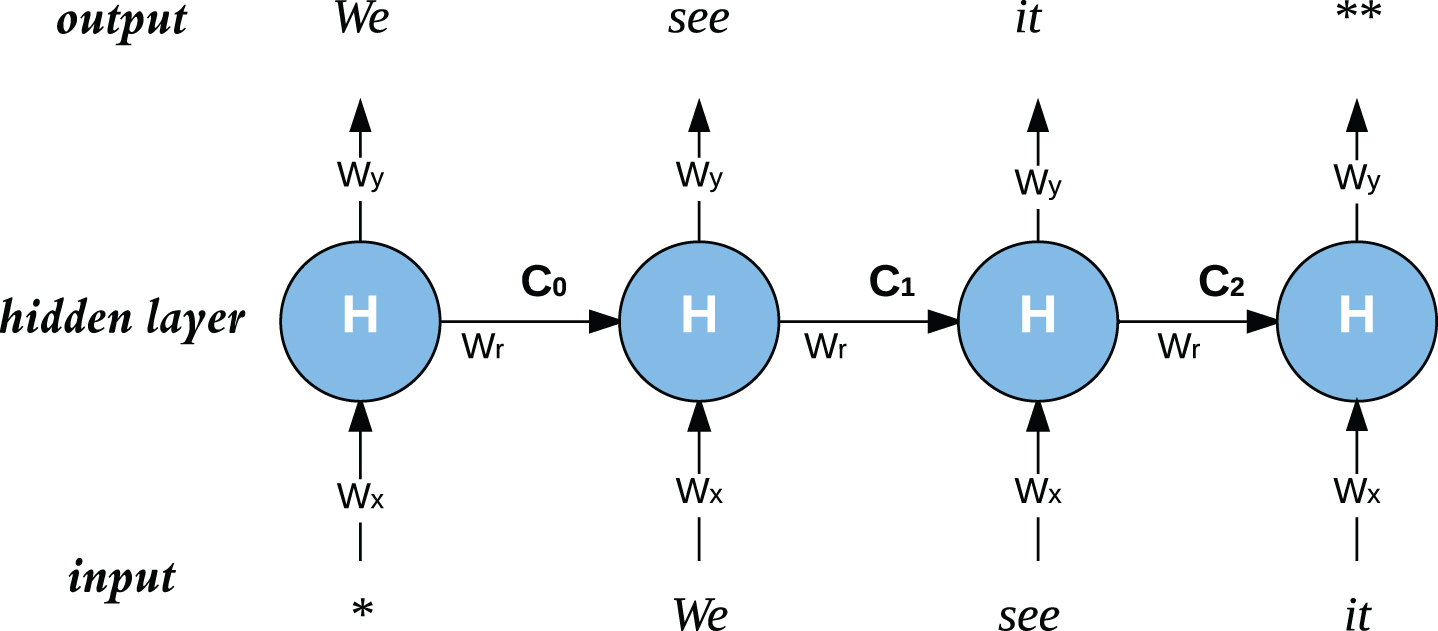
Example of a Recurrent Language Model.

2.2.1 Training and backpropagation

Given a text corpus with variable-length sentences, s¹, s², . . . , s^N, the learning objective for a language model is to minimize the cross-entropy loss of the given text corpus.

$J (θ) = \sum_{i = 1}^{N} - log p (s^{i})$ (3)

The RNN language model learning is commonly performed using stochastic gradient descent (SGD) algorithm. The gradient is computed over a subset of training samples (mini batches). We update weights after every mini-batch gradient computation (also called minibatching). The mini-batch SGD results into less computation as compared to the full-batch (all training samples at once) or online learning. The simplest update equation for updating weight is:

$θ = θ - η \frac{δ J (θ)}{δ θ}$ (4)

The gradient of the cost function ( $\frac{δ J (θ)}{δ θ}$ ) points in the direction of maximum ascent, but in order to minimize the cost function, it should move to the opposite direction. The learning rate, η, quantifies the step-size for each mini-batch iteration. A very small learning rate may end up in local minima, or a very large learning rate may overshoot and jump out off global minima.

To compute the gradient for overall loss, J (θ), we first need to derive gradient at each time step, J_t (θ) = - log p_t (s^(t)), with respect to all RNN weights (W_r, W_x, W_y) as well as inputs. We’ll illustrate the backpropagation process by computing gradient for a single time step.

Let’s start at time t = 2 and compute gradient with respect to W_x using chain rule:

$\frac{δ J_{2}}{δ W_{x}} = \frac{δ J_{2}}{δ y_{2}} \frac{δ y_{2}}{δ c_{2}} \frac{δ c_{2}}{δ W_{x}}$ (5) using (1), we have, $c_{2} = f (W_{x} x_{2} + W_{r} c_{1})$

That means, cell state at t = 2, in addition to W_x, also depends on cell state at t = 1. Considering this, from Fig. 4, we have,

Fig.4

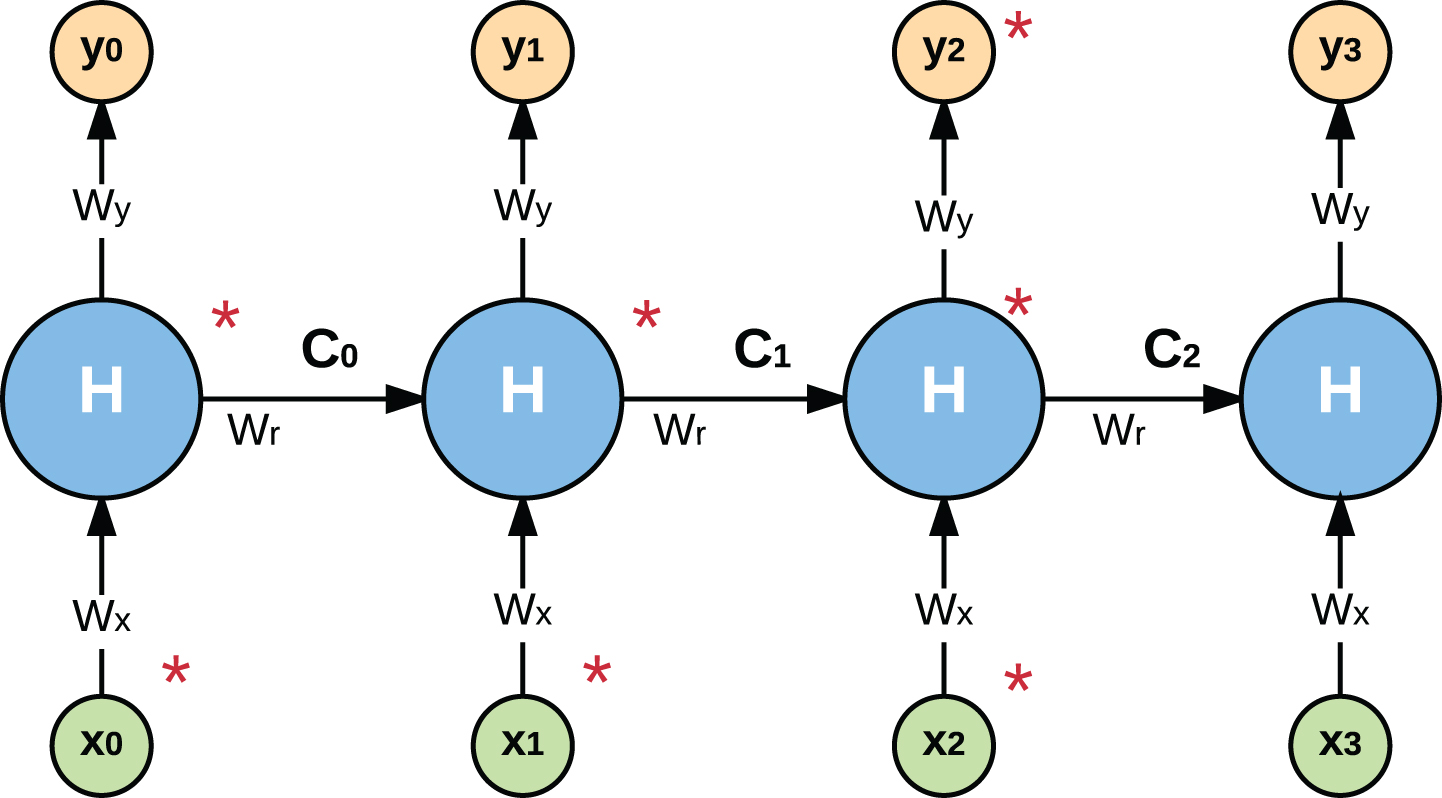
Backpropagation through time with repect to W_x.

$\frac{δ c_{2}}{δ W_{x}} = \frac{δ c_{2}}{δ c_{1}} \frac{δ c_{1}}{δ W_{x}} + \frac{δ c_{1}}{δ c_{0}} \frac{δ c_{0}}{δ W_{x}}$ (6)

Combining (5) and (6), we get the total backpropagation at t = 2 as,

(See the starred path in Fig. 4),

$\frac{δ J_{2}}{δ W_{x}} = \sum_{j = 0}^{2} \frac{δ J_{2}}{δ y_{2}} \frac{δ y_{2}}{δ c_{2}} \frac{δ c_{2}}{δ c_{j}} \frac{δ c_{j}}{δ W_{x}}$ (7)

Equation (7) can be generalized for any time-step and written as,

$\frac{δ J_{t}}{δ W_{x}} = \sum_{j = 0}^{t} \frac{δ J_{t}}{δ y_{t}} \frac{δ y_{t}}{δ c_{t}} \frac{δ c_{t}}{δ c_{j}} \frac{δ c_{j}}{δ W_{x}}$ (8)

In a similar way as Equation (8), we can back-propagate in time with respect to all other RNN weights.

2.2.2 Long Short Term Memory

Despite the fact that recurrent neural network gradient computation is pretty straightforward, it suffers from two major drawbacks:

Exploding gradient

Vanishing gradient

The exploding gradient refers to the phenomenon when gradient values become exponentially large as we back propagate through time (BPTT). The exploding gradient problem is solved by clipping the gradient after it reaches a certain threshold values. The vanishing gradient on the other hand is a challenging task and it occurs when gradient values starts approaching zero as we BPTT. Vanishing gradient forces our network to become more biased toward shorter range dependencies because gradient values for further back time steps becomes insignificant. There are certain ways to solve the vanishing gradient problem, such as, specific leaky generators [14], regularization [15], and long-short term memory [16] etc.

The Long Short Term Memory (LSTM) by [16] is most widely used solution for gradient vanishing problem. LSTMs can be used to model longer range dependencies more efficiently than RNNs. In contrast with RNNs, where each cell is just a single activation function like sigmoid, tanh etc., LSTMs has more than just a single activation function. Figure 5 depicts a slightly abstract difference between RNN and LSTM. The brief steps involved in the working of basic LSTM network are 5 ,

First, we decide which information we need to discard. This decision is made by “forget layer”. It is a simple sigmoid function.

Then we make decision on information to be stored in cell state. A sigmoid layer chooses which values to update. Then a tanh layer creates a vector which could be added to the cell state. At the end, these two values are combined to make final update to the cell state.

Finally, the decision over which parts of the cell state will proceed to output is made using a sigmoid function in output layer.

Fig.5

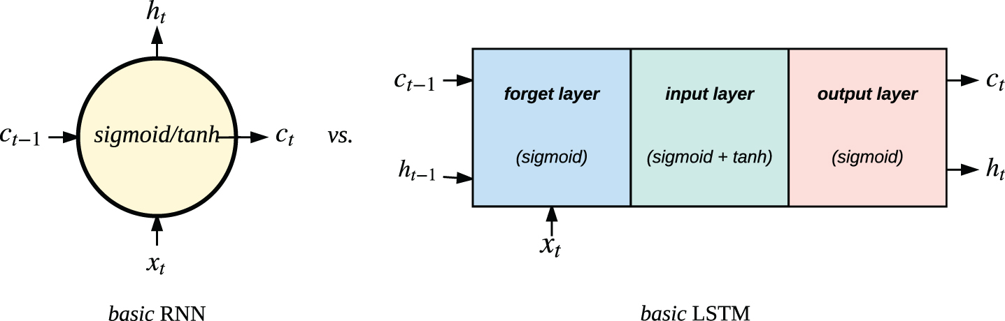
Comparison among basic RNN and LSTM.

There are many components in the LSTM training pipeline which works exactly as RNNs. In addition to this similarity, LSTM training pipeline has additional components such as forget layer, input layer, output layer etc.

3 Neural Machine Translation

Having introduced the major components of NMT pipeline. We can now proceed our discussion on neural machine translation. Given a parallel corpus, T, of source language sentences (x) and target language sentences (y), a neural machine translation system models the conditional probability p (y/ - x). This goal is achieved by an encoder-decoder architecture (discussed in Section 2).

More formally, encoder computes an embedding (or representation), e, for every source sentence. Decoder decomposes the log conditional probability based on this representation and hence generates a translation. The log conditional probability is given as:

$log p (y / x) = \sum_{t = 1}^{m} log p (y_{t} / y_{1} - y_{t - 1}, e)$ (9)

Neural machine translation has attained state of the art performances in many language pairs such as English-French, English-German etc. As mentioned earlier, most common neural network to use for sequential data (a sentence in our case) is RNN. In recent NMT systems, RNNs differs in terms of depth (single or multiple layers), type (gated recurrent units, long short-term memory) and directionality (unidirectional or bidirectional). The most successful NMT systems in recent years have used deep RNNs with LSTMs as the recurrent units. The choice of LSTMs depends heavily on their many advantages over RNNs which were discussed in previous section. An example of a deep multi-layer network architecture for translating a source language sentence (English) to a target language sentence (Punjabi) is depicted in Fig. 6. The following points illustrates the translation process followed in the above architecture,

The bottom layer receives a source sentence (as discrete words) followed by a special symbol (*) which indicates the end of sentence as well as progress from encoder to decoder, and a target sentence. Given these words, model retrieves the corresponding representation (embedding layer).

The retrieved representations are then fed to the two (encoder and decoder) multi-layer LSTM network.

The starting state of the encoder is initialized using zero vector whereas decoder is initialized using last state of the encoder.

Finally, the output from the top hidden layer at the decoder side is transformed using softmax into a probability distribution over the target vocabulary and a translation is retrieved.

Fig.6

Translation example using neural machine Translation architecture.

3.1 Neural Machine Translation with attention

Despite the excitement with neural machine translation, it is still difficult to predict long-range dependencies. The bottleneck being the fixed length encoding we fed to the decoder. The idea to overcome this bottleneck is to allow the model to automatically attend to the words of a source sentence which are more relevant for the prediction of present target word. This approach has been successfully applied for neural machine translation by [9] and [17].

To be able to attend over specific words of a source sentence, vectors of each word in a sentence are maintained instead of single vector for whole sentence. The number of vector for a source sentence (h_{s
₁} . . . h_{s
_t}) depends on number of words in the sentence. These words (or their corresponding vectors) can be concatenated to form a matrix H_s as: $H_{s} = [h_{s_{1}}; h_{s_{2}}; . . h_{s_{t}}]$

Every column in H_s corresponds to a word in source sentence. The matrix will have variable number of columns depending on the number of words in source sentence. To compute the probabilities over the vocabulary on decoder side, a vector is required instead of a matrix. To achieve this, we compute an attention vector (a_t) which transforms the matrix H_s into a vector. It is like calculating a weighted average. This attention vector decides how much weightage we give to particular source words to generate current target word.

The components of attention vector are the attention scores we assign to each column of matrix H_s. These attention scores are calculated using current target state vector (h_t) and source states (or column vectors of H_s). There are several way to compute these attention scores such as simple dot product approach by [17] and using multilayer perceptrons by [9]. For English-Punjabi language pair, we tried attention mechanism by [17].

3.2 Training

The training objective of NMT system is quite similar to a recurrent language model (Equation 3), except we condition the target sentence on source sentence. The loss function for neural machine translation training over the parallel corpus T is formulated as:

$J = \sum_{(x, y) \in T} - log p (y / x)$ (10)

The forward propagation for the neural machine translation architecture is nearly similar to that of ordinary recurrent neural networks. The only difference is, we initialize the decoder side stacked LSTM cells by using the representations from the encoder side.

The back propagation at decoder side is similar to any regular recurrent neural network. To migrate from decoder to encoder, the last decoder cell state gradient is passed back to encoder. Then, back propagation algorithms continues through the encoder side in a similar way but without prediction loss.

3.3 Testing

After training our NMT system, we test it for new (unseen) source sentences. There are two main methods to accomplish this such as Greedy decoding and Beam search decoding. The greedy decoding approach generate predictions at every time step. The NMT beam-search is simpler than the beam-search algorithm used in phrase based statistical machine translation systems. In a slightly abstract way, beam-search algorithm for NMT system works in a following way, (κ being the beam size (2,3,5 etc.))

At every time step, we keep trace of top κ translations.

Instead of making a greedy choice (picking the most likely word), we pick the top κ most likely words.

We combine top κ translations with top κ most likely words and generate new set of translations $\tilde{κ}$ .

This simple beam-search approach delivers a substantial improvement in the translation quality.

4 Dataset description

A good parallel corpus plays a vital role in all the machine translation approaches. In the context of Indian languages, especially English-Punjabi, there is scarcity of parallel corpora. The available parallel corpus for English-Hindi includes Technology Development for Indian Language (TDIL) corpus, EMILLE corpus, Open source parallel corpus (OPUS).

The TDIL corpus includes domain specific corpus for domains like health, tourism, agriculture and entertainment. Despite the fact that there are four domains, the number of sentences per domain are very less. There are also several mismatches between parallel sentences which acts as a noise for the parallel corpus. It even includes several sentences from Malayalam language other than Punjabi.

The OPUS contains localization files of GNOME, Ubuntu and KDE4. Most of the sentences are just repetitions. Considering the noise and less number of sentences in TDIL corpus and OPUS, it is not appropriate for even a baseline NMT system. To build a decent NMT system, we crawled data from various freely available websites. The entire corpus was further cleaned and grammatical errors/typos were corrected. We restricted every sentence of our parallel corpus to have atleast 4 words. The final statistic of the dataset that we used to train our NMT system is mentioned in Table 1.

Table 1
Final statistic of training data

S no. Dataset # of sentence pairs

1 OPUS^* 6730

2 TDIL 64410

3 Crawled data 71660

Total 1,42,800

S no.	Dataset	# of sentence pairs
1	OPUS^*	6730
2	TDIL	64410
3	Crawled data	71660
Total	1,42,800

^*Open Source Parallel Corpus.

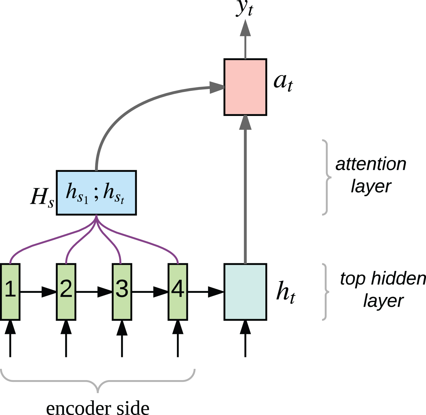
The details of the training data used are mentioned in Table 2. The test and development dataset had 488 and 300 sentences respectively. The version-1 of this dataset is available at our Github repo 6 .

Fig.7

Intuitive illustration of global attention.

Table 2

Details of the English-Punjabi Training data

Language	Number of sentences	Vocabulary size	Average sentence length
English	1,42,833	55,540	14.32
Punjabi	1,42,833	78,062	15.25

5 Experiment and results

To evaluate the system, BLEU scores on tokenized translations were used. The NMT system was implemented using [18] on a Tesla K40c GPU. We tried two variants of parallel corpora; one with simple tokenized sentences and another with Byte Pair Encoding (BPE) by [19]. The BPE was learned on concatenation of train data with 40000 merge operations. The attention mechanism by [17] was used for training the system. The BLEU scores for the system along with some important hyperparameters are reported in Table 3. The hyperparameter “bi” stands for birectional RNNs. Even though the word order

Table 3
Evaluation of English-Punjabi NMT system

S. no.	Input	Encoder	Layers	Units	Beam width	BLEU
1	tokenized	bi	4	512	10	24.48
2	BPE	bi	4	512	10	26.07

of English and Punjabi is different, NMT framework seems to learn this without any external re-ordering module.

The other important hyperparameters used for training the NMT system are:

Number of training steps: 25000

Optimizer: SGD

Batch size: 128

Dropout: 0.2

Initial learning rate: 1

Decay factor 7 : 0.85

Start decay step 8 : 13000

Decay steps 9 : 3000

The sample translations of our best system (S. no. 2 in Table 3) and other existing systems are given in Fig 8. The errors (grammatical/syntactical) in the translated output are marked with bold letters. The translations generated by our system are adequate as well as fluent. It also preserved the line ending character (|) for all the translations unlike Google Translate and AnglaMT.

Fig.8

Example translation of our system compared with Google Translate and AnglaMT system.

Google Translate and AnglaMT are the only existing systems for English to Punjabi translation. In order to quantify our systems perormance, we manually translated our test dataset using AnglaMT and Google Translate and then computed BLEU scores for translated sentences. The BLEU scores obtained for these systems along with our best system are reported in Table 4. This comparison is just to quantify the performances among these systems.

Table 4

Comparison with other systems

S no.	System	BLEU
1	AnglaMT	05.97
2	Google Translate	11.09
3	ours	26.07

6 Conclusion and future work

This work applies attention based neural machine translation to English-Punjabi language pair. The system was trained in an end-to-end manner without having to learn additional components as in statistical machine translation. The system generated adequate and fluent translations. The NMT framework also learned the word order each language. Punjabi language is syntactically as well as grammatically quite similar to Hindi. Moreover, they also share almost the same vocabulary. That means, the same system can be used for training over a English-Hindi parallel text corpus. As a future work, we plan to collect more parallel corpus to enhance the system performance and cover more vocabulary. An English-Punjabi dictionary can also be incorporated to translate out-of-vocabulary (OOV) words while decoding.

Footnotes

Reduce learning rate by this factor.

Start reducing learning rate at this step number.

Keep reducing learning rate after each decay steps.

References

Shapiro

S.C.

, Encyclopedia of artificial intelligence2, John, 1992.

Weaver

, Translation, Machine Translation of Languages14 (1955), 15–23.

Brown

P.F.

, Pietra

V.J.D.

, Pietra

S.A.D.

and Mercer

R.L.

, The mathematics of statistical machine translation: Parameter estimation, Computational Linguistics19(2) (1993), 263–311.

Koehn

, Statistical machine translation, 2009Cambridge University Press.

Och

F.J.

and Ney

, Discriminative training and maximum entropy models for statistical machine translation, Association for Computational Linguistics, In Proceedings of the 40th Annual Meeting on Association for Computational Linguistics, 2002, pp. 295–302.

Sutskever

, Vinyals

and Le

Q.V.

, Sequence to sequence learning with neural networks, In Advances in Neural Information Processing Systems (2014), pp. 3104–3112.

Antony

P.J.

, Machine translation approaches and survey for Indian languages, Computational Linguistics and Chinese Language Processing18(1) (2013), 47–78.

Sinha

R.M.K.

, Jain

and Jain

, Translation from english to indian languages: Anglabharti approach, In Proceeding of the Symposium on Translation Support System (2001), pp. 15–17.

Bahdanau

, Cho

and Bengio

, Neural machine translation by jointly learning to align and translate.2014arXiv preprint arXiv: 1409.0473.

10.

, Schuster

, Chen

, Le

Q.V.

, Norouzi

, Macherey

, Krikun

, Cao

, Gao

, Macherey

, et al., Google’s neural machine translation system: Bridging the gap between human and machine translation, 2016arXiv preprint arXiv:1609.08144.

11.

Gehring

, Auli

, Grangier

, Yarats

and Dauphin

Y.N.

, Convolutional sequence to sequence learning. In, Precup

Doina

and Whye Teh

Yee

, editors, Proceedings of the 34th International Conference on Machine Learning, volume 70 of Proceedings of Machine Learning Research, International Convention Centre, Sydney, Australia, 2017, pp. 1243–1252. PMLR.

12.

Mikolov

, Karafiát

, Burget

, Cernocký

and Khudanpur

, Recurrent neural network based language model, In Interspeech2 (2010), 3.

13.

Mikolov

, Kombrink

, Burget

and Cernocký

, and Khudanpur

, Extensions of recurrent neural network language model, In Acoustics, Speech and Signal Processing (ICASSP), 2011 IEEE International Conference on (2011), pp. 5528–5531IEEE.

14.

Jaeger

and Lukosevičius

, Popovici

and Siewert

, Optimization and applications of echo state networks with leaky-integrator neurons, Neural networks20(3) (2007), 335–352.

15.

Pascanu

, Mikolov

and Bengio

, On the difficulty of training recurrent neural networks, ICML28(3) (2013), 1310–1318.

16.

Hochreiter

and Schmidhuber

, Long short-term memory, Neural Computation9(8) (1997), 1735–1780.

17.

Luong

M.-T.

, Pham

and Manning

C.D.

, Effective approaches to attention-based neural machine translation, In Proceedings of the 2015 Conference on Empirical Methods in Natural Language Processing, Lisbon, Portugal, 2015, pp. 1412–1421. Association for Computational Linguistics.

18.

Luong

M.-T.

, Brevdo

and Zhao

, Neural machine translation (seq2seq) tutorial. https://github.com/tensorflow/nmt, 2017.

19.

Sennrich

, Haddow

and Birch

, Neural machine translation of rare words with subword units.arXivpreprint arXiv:1508.07909, 2015.