A simple hybrid approach to recognizing textual entailment

Abstract

We explore various machine learning-based classifiers applied to rule-based features for recognizing textual entailment. The features, extracted with a set of synthesized matching rules, reflect syntactic and semantic similarity between the text and the hypothesis. The fact that we use only seven relatively simple features makes our method suitable for low-resource languages. We test our method on the test sets of the RTE competitions and achieve accuracy of up to 69.13%.

Keywords

Textual entailment dependency parsing semantic similarity supervised machine learning RTE datasets

1 Introduction

Recognizing Textual Entailment (RTE) is a major challenge in natural language processing (NLP). Due to its applications in many NLP domains, such as information retrieval, information extraction, question answering [1], paraphrase acquisition, text summarization, reading comprehension, and machine translation, a number of RTE challenges have been organized by the PASCAL Network of Excellence, funded by the European Union, for many years.

RTE is the task of, given a pair of text snippets as input, deciding whether the meaning of one fragment (hypothesis, H) can be most likely inferred from the meaning of the other fragment (text, T) as would typically be interpreted by people. This establishes a directional relationship that holds from T to H (T entails H), but not necessarily from H to T (H does not necessarily entail T), as in the following example:

Example 1. T: Iran will soon release eight British servicemen detained along with three vessels. H: British servicemen detained.

We present a hybrid method for solving the RTE task, which combines a small number of rule-based features with decision-making based on machine learning (ML). After pre-processing, the T– H pair is passed to a dependency parser to obtain a dependency graph structure. Next, a set of features is extracted to train a classifier to predict whether T entails H. This set of features includes summation of in-degree and out-degree of the nodes in the H’s dependency graph, named entity-matched ratio, antonym bit, negation bit, superlative degree modifier bit, and an overall entailment score. The features are calculated by a synthesized set of matching rules, which mainly reflect syntactic divergence augmented with semantic similarity measures. We test different combinations of our features on several ML-based classification algorithms available in the WEKA toolkit.

The paper is organized as follows. Section 2 discusses related work. Section 3 gives an overview of our method. Section 4 presents our feature set. Section 5 gives the experimental results. Section 6 presents error analysis. Section 7 concludes the paper.

2 Related work

A number of RTE methods have been reported in the literature. Some of them represent the text and hypothesis as syntactic dependency-parse trees and compare them to find out the degree of inclusion of H’s tree into T’s tree [2]. Many systems use some simple form of lexical matching such as n-gram matching, percentage of word overlap, longest common subsequence, or skip-gram matching. Some systems also use some form of semantic techniques such as semantic role labelling [3], atomic propositions [4], inference rules, universal networking language augmented with semantic similarity measures [5], etc. Recently, supervised classification techniques have become the predominant approach to the RTE task. ML-based techniques use text features classify the T– H pairs into those with and without entailment.

Rios and Gelbukh [6] assume entailment if the Levenshtein distance between T and H is below a threshold. Kouylekov and Magnini [7] use tree edit distance. Marsi et al. [8] use alignment of T and H dependency trees for the entailment decision. Herrera et al. [9] parse the T– H pair using Lin’s Minipar and then find a lexical entailment between each word in the hypothesis with some word in the text using WordNet relations such as synonymy, hyponymy, and antonymy to calculate the degree of inclusion of H in T. Blake [10] explores the degree to which the sentence structure plays a role in detecting textual entailment.

Pakray et al. [11] compare various features, including semantic roles, of syntactic structures of T and H. They use different weights for exact and partial matches. The weights are summed up and compared with a threshold to make the entailment decision. These authors also use anaphora resolution [12] and a combination of lexical, syntactic, and semantic features [13]. Dinu and Wang [14] use an inference rule-based technique. They start with a collection of inference rules acquired automatically basing on the distributional hypothesis and refined by obtaining more rules using a handcrafted lexical resource.

Malakasiotis and Androutsopoulos [15] use four support vector machines (SVM), one per subtask of the RTE3 challenge, with features based on string similarity measures at the lexical and shallow syntactic level. MacCartney et al. [16] use 28 features, such as polarity, adjuncts, antonymy, and factivity, to train a logistic regression classifier. Szpektor and Dagan [17] learn entailment rules for unary templates in an unsupervised way, using dependency parse trees. Mirkin et al. [18] use an integrated approach: they acquire the candidate entailment, construct a feature set for all candidates using pattern-based and distributional information, and train SVM on these features to integrate systemically different feature types.

Li et al. [19] extract features such as lexical semantic similarity, named entities, average distance, dependent content word pairs, text length, negation, etc. from the T– H pairs of the RTE3 dataset and run a decision tree (J48) on several feature combinations. Pham et al. [20] use features such as the longest common subsequence of T and H, word overlap, Levenshtein distance, named entity match, polarity match, etc., to train an SVM classifier. Zanzotto et al. [21] use supervised ML to derive first-order rewrite rules from annotated examples. Agichtein [22] use categories of features such as lexical similarity (word overlap, cosine similarity, substring similarity, etc.), syntactic similarity (mainly role similarity and POS similarity), and semantic similarity (several WordNet similarity measures such as Resnik, Lin, and Wu-Palmer measures, etc.) to train ML-based classifiers such as J48, SMO, and Naïve Bayes.

Saikh et al. [23] use as features a number of lexical and vector-based similarity measures, plus two machine-translation evaluation metrics: BLEU and METEOR. They use several feature combinations to train ML-based classifiers such as SMO, AdaBoostM1, J48, LibSVM, etc. Rios et al. [24] use a cosine similarity measure and a causal non-symmetric measure as features for ML, obtaining best results with SVM and Naïve Bayes classifiers. Castillo [25] trains a SVM classifier on a variety of lexical and semantic features such as TF-IDF measure, Jaro– Winkler distance, and Euclidean distance.

Basak et al. [26, 27] make the entailment decision by comparing the dependency tree structures of T and H based on a number of dependency triple matching rules manually extracted from the RTE datasets. In [26], for a matching T triple for an H dependency triple, a matching score in the range of [– 1, 1] is assigned to the dependent node associated with that H triple. Finally, the H dependency tree is traversed in level order from the bottom level and the scores of the nodes are calculated and propagated to the upper levels. The entailment score between the T– H pair is obtained at the root node of the tree at the end of the traversal process. In the present paper, we mainly use the features designed with matching rules described in [26].

3 Outline of the method

Our experiments included the following steps: pre-processing, dependency parsing, lexical alignment (using WordNet 2.1 and a stemmer), dependency graph representation, feature selection and analysis (using named entity tags and a set of matching rules), and entailment classification (using a combination of features and an ML-based classifier). Subsequent subsections illustrate the individual components.

3.1 Pre-processing

Before the actual TE recognition process is invoked, each T– H pair is fed to a number of pre-processing phases illustrated below.

Breaking hyphenated words. The RTE datasets include T– H pairs where one of T or H contains hyphenated words, while the other does not. Such hyphenated words cause problems in the lexical alignment phase. It is necessary to break those words to their component words by removing the hyphens.

Normalization. We normalize numeric expressions by removing the comma, such as “8,568” to “8568”.

Replacement of special symbols. We replace some special symbols by the expanded terms, e.g., “% ” is replaced by “percent”, “$” by “dollar”, etc. A symbol is replaced in T (or H) only if its expanded form is present in H (or T); otherwise, it remains unchanged.

Expansion of contracted tokens. This step checks the occurrence of contracted tokens in the text and hypothesis and replaces them by their corresponding expanded forms. For example, I’ve is replaced by I have, he’ll is replaced by he will etc.

Merging multiple sentences. Often the text T consists of various sentences, resulting in a short paragraph. Since we use a single dependency graph, we merge the sentences in the paragraph by replacing the intermediate full stops with hyphen (–).

NE tagging. Each of the text and hypothesis is subjected to a named entity recognizer (NER) which assigns an NE tag to the named entities present in the T– H pair. A token can be tagged as any of the several types of Named Entity such as PERSON, LOCATION, ORGANIZATION, DATE etc.

3.2 Feature extraction and classification

Dependency parsing. Each of the text fragments of the processed T– H pair is passed on to this phase of dependency parsing. The output of this phase is a set of dependency triples of form R (W₁, W₂) where W₁ and W₂ are two tokens of a sentence associated by the relation labelled as R.

Lexical alignment. This phase aims to lexically align each token $W_{H}^{j}$ of H with one or more tokens $W_{T}^{i}$ of T, producing a set of lexically aligned token pairs ( $W_{H}^{j}$ , $W_{T}^{i}$ ), where the token $W_{H}^{j}$ is aligned to the token $W_{T}^{i}$ by any of the WordNet relations as, e.g., a synonym, hypernym, hyponym, derivationally related form, entailment, cause, or antonym. For this, all T and H tokens were stemmed before the alignment process. Consider the following T– H pair:

Example 2. T: The person is the founder of the company. H: The man founded the company.

After stemming of both T and H, the lexical alignment between the token pairs is performed; see Fig. 1. The arrows represent the alignment between the corresponding tokens of H with one or more tokens of T, and colors indicate different WordNet relations by which the tokens are associated. However, one hypothesis token may be lexically aligned to more than one text token. The dashed lines are used in the diagram to indicate one-to-many mappings and the thick lines indicate the one-to-one mappings.

Fig.1

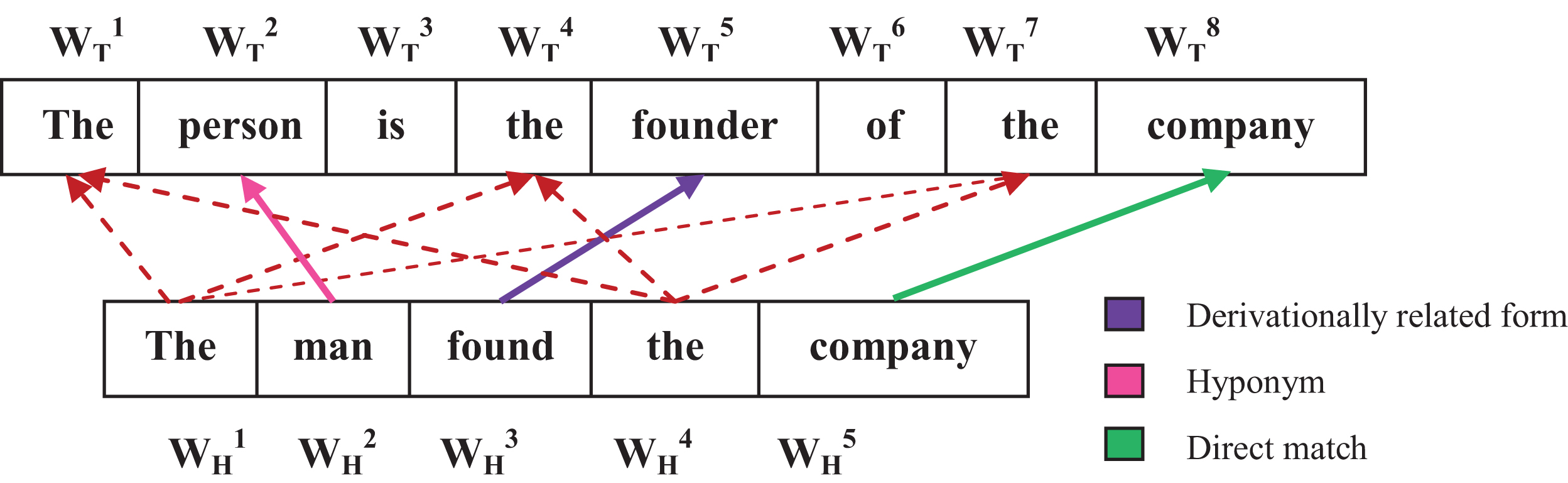
Lexical alignment between text and hypothesis tokens.

Dependency graph. After each of the text and hypothesis is parsed by the dependency parser, all the dependency triples are joined together to form a graph like structure. Each triple R (W₁, W₂) is represented as an arc in the dependency graph connecting two nodes W₁ and W₂ labelled by the relation R.

Feature selection and analysis. The features for the final classification are explained in the next section.

Entailment classification. The values of the seven features are extracted from the RTE devsets on which several ML-based classifiers were trained. The classifiers are run on different combination of the features extracted from the datasets. Two-way (yes or no) entailment decisions are cast as a classification problem. We tested various classification algorithms such as Logistic, Simple Logistic, J48, Multilayer Perceptron, LogitBoost, SMO, AdaBoost, NaiveBayes, BayesNet with different feature combinations.

4 Feature selection and analysis

The features we used are summarized in Table 1.

Table 1
Features used in our experiments

Feature Name

F1 Sum of in_degree of vertices of H dependency graph

F2 Sum of out_degree of vertices of H dependency graph

F3 Named entity matched ratio

F4 Antonym bit

F5 Negation bit

F6 Superlative degree modifier bit

F7 Entailment score

Feature	Name
F1	Sum of in_degree of vertices of H dependency graph
F2	Sum of out_degree of vertices of H dependency graph
F3	Named entity matched ratio
F4	Antonym bit
F5	Negation bit
F6	Superlative degree modifier bit
F7	Entailment score

4.1 Sum of in_degree (F1) and out_degree (F2) of H

Each node in the H dependency graph is assumed to have six score components of in_degree and out_degree, as summarized in Table 2.

Table 2
Assignment of values on the in_degree and out_degree components of the hypothesis graph

Component Assigned values

total_in_degree (in_t) Total number of incoming edges (arrow heads) falling on a node

total_out_degree (out_t) Total number of outgoing edges (arrow tails) emitting from a node

matched_in_degree (in_m) Summation of the matching scores on all incoming edges

matched_out_degree (out_m) Summation of the matching scores on all outgoing edges

average_in_degree (in_a) Dividing in_m by in_t

average_out_degree (out_a) Dividing out_m by out_t

Component	Assigned values
total_in_degree (in_t)	Total number of incoming edges (arrow heads) falling on a node
total_out_degree (out_t)	Total number of outgoing edges (arrow tails) emitting from a node
matched_in_degree (in_m)	Summation of the matching scores on all incoming edges
matched_out_degree (out_m)	Summation of the matching scores on all outgoing edges
average_in_degree (in_a)	Dividing in_m by in_t
average_out_degree (out_a)	Dividing out_m by out_t

After generating the dependency graph by combining all dependency triples, the in_t and out_t components of each node are calculated by counting their incoming and outgoing edges. The components in_m and out_m are calculated using various matching criteria. Each H dependency triple R_H (W₁, W₂) is compared with all T triples. When a matching triple is found, a matching score in the range [– 1,1] is assigned to in_m and out_m components of the H nodes W₂ and W₁, respectively, by synthesizing a set of matching rules from [26] built by analyzing the development sets of RTE. The process can be illustrated by an example from the RTE1 development set, with dependency triples shown in Table 3:

Table 3

Dependency triples of the T– H pair of Example 3

T dependency triples	H dependency triples
T1: nsubj(killed-2, Guerrillas-1)	H1: nsubj(killed-2, Guerrillas-1)
T2: root(ROOT-0, killed-2)	H2: root(ROOT-0, killed-2)
T3: det(peasant-4, a-3)	H3: det(civilian-4, a-3)
T4: dobj(killed-2, peasant-4),	H4: dobj(killed-2, civilian-4)
T5: det(city-7, the-6)
T6: prep_in(killed-2, city-7)
T7: prep_of(city-7, Flores-9)

Example 3. T: Guerrillas killed a peasant in the city of Flores. H: Guerrillas killed a civilian.

Table 4 shows the matching between the H and T dependency triples according to the matching rules from [26]. The last two columns show the values of matched_in_degree (in_m) and matched_out_degree (out_m) components assigned to each node in the H dependency graph. Table 5 summarizes the values of the six score components of each node after matching. The H dependency graph is as follows:

Guerilla \overset{nsubj}{\leftarrow} kill \overset{dobj}{\to} peasant \overset{det}{\to} a

Table 4

Simulation of matching between the T– H dependency triples of Example 3

H triple	T triple	Matching rule	in_m		out_m
			Value	Node	Value	Node
H1	T1	1	1	Guerilla	1	kill
H2	—	—	—	—	—	—
H3	—	7	1	a	1	civilian
H4	T4	Category 2 of semantic similarity matching module	0.7619	civilian	0.7619	kill

Table 5

Score components of each node in of Example 3

Node	in_t	out_t	in_m	out_m	in_a	out_a
Guerrilla	1	0	1	0	1	0
kill	0	2	0	1 + 0.7619	0	(1 + 0.7619)/2 = 0.8809
a	1	0	1	0	1	0
civilian	1	1	0.7619	1	0.7619	1

with the score components of in_t, out_t, in_m, out_m, in_a, out_a being as follows: Guerilla (1, 0, 1, 0, 1, 0), kill (0, 2, 0, 1.7619, 0, 0.8809), peasant (1, 1, 0.7619, 1, 0.7619, 1), a (1, 0, 1, 0, 1, 0). Finally, the two feature values summation of in_degree F1 and summation of out_degree F2 are calculated as

\begin{matrix} F 1 & = & \frac{\sum in_a}{# of nodes with in_t \neq 0} \\ = & \frac{(1 + 1 + 0.7619)}{3} = 0.9206, \\ F 2 & = & \frac{\sum out_a}{# of nodes with out_t \neq 0} \\ = & \frac{(0.88 + 1)}{2} = 0.94 . \end{matrix}

4.2 Named entity-matched ratio (F3)

Named entities (NE) are important information carriers in text. It is a general assumption that each NE of the hypothesis H must be contained in the text T in order to be entailed by T. Otherwise it is very likely that H cannot be entailed from T.

This feature calculates the ratio of the number of NEs common between the text and the hypothesis to the total number of NEs in the hypothesis. If the hypothesis does not contain any named entities, this ratio is set to 1.

If NE_S(T) and NE_S(H) indicate the set of named entities in the text and hypothesis respectively, the named entity matched ratio is $F 3 = \frac{| NE_S (T) \cap NE_S (H) |}{| NE_S (H) |}$ where NE _ S (T) ∩ NE _ S (H) is the number of named entities common between T and H.

Consider a T– H pair as example with the named entities being highlighted in bold fonts.

Example 4. T: John and Sam are students of the same college. H: John and Mary are students of the same college.

Here NE_S(T) = {John, Sam} and NE_S(H) = {John, Mary}, which indicates |NE _ S (T) ∩ NE _ S (H) |=1. Therefore this ratio for the given T– H pair is 0.5.

4.3 Antonym bit (F4)

If any hypothesis dependency triple R_H (W₁, W₂) matches with any of the text triples according to matching rule 4 from [26], then a score of – 1 is assigned to the in_m component of the node W₂ and to the out_m component of the node W₁. Negative scores are assigned to the in_m and out_m components of hypothesis nodes W₂ and W₁ in order to lower the values of the feature variables F1 and F2 aiming to classify the T– H pair as a case of no entailment. Moreover, it also sets the value of an antonym bit (Feature F4) to 1. By default (on detecting no antonymy), the value of this bit is set to 0.

An example T– H pair from the RTE development set is presented in Example 5 to show how the presence of antonym between a text– hypothesis pair affects the values of the feature variables F1 and F2:

Example 5. T: Doug Lawrence bought the impressionist oil landscape by J. Ottis Adams in the mid-1970s at a Fort Wayne antiques dealer. H: Doug Lawrence sold the impressionist oil landscape by J. Ottis Adams.

Some of its dependency triples are presented in Table 6. The tokens bought– sold are antonyms (in fact, conversives). The matching between the T and H dependency triples according to the synthesized rules as presented in [26] is provided in Table 7.

Table 6
Dependency triples of the T– H pair of Example 5

T dependency triples H dependency triples

T1: nn(Lawrence-2, Doug-1) H1: nn(Lawrence-2, Doug-1)

T2: nsubj(bought-3, Lawrence-2) H2: nsubj(sold-3, Lawrence-2)

T3: root(ROOT-0, bought-3) H3: root(ROOT-0, sold-3)

T4: det(landscape-7, the-4) H4: det(landscape-7, the-4)

T5: amod(landscape-7, impressionist-5) H5: amod(landscape-7, impressionist-5)

T6: nn(landscape-7, oil-6) H6: nn(landscape-7, oil-6)

T7: dobj(bought-3, landscape-7) H7: dobj(sold-3, landscape-7)

T8: nn(Adams-11, J.-9) H8: nn(Adams-11, J.-9)

T9: nn(Adams-11, Ottis-10) H9: nn(Adams-11, Ottis-10)

T10: prep_by(bought-3, Adams-11) H10: prep_by(sold-3, Adams-11)

T dependency triples	H dependency triples
T1: nn(Lawrence-2, Doug-1)	H1: nn(Lawrence-2, Doug-1)
T2: nsubj(bought-3, Lawrence-2)	H2: nsubj(sold-3, Lawrence-2)
T3: root(ROOT-0, bought-3)	H3: root(ROOT-0, sold-3)
T4: det(landscape-7, the-4)	H4: det(landscape-7, the-4)
T5: amod(landscape-7, impressionist-5)	H5: amod(landscape-7, impressionist-5)
T6: nn(landscape-7, oil-6)	H6: nn(landscape-7, oil-6)
T7: dobj(bought-3, landscape-7)	H7: dobj(sold-3, landscape-7)
T8: nn(Adams-11, J.-9)	H8: nn(Adams-11, J.-9)
T9: nn(Adams-11, Ottis-10)	H9: nn(Adams-11, Ottis-10)
T10: prep_by(bought-3, Adams-11)	H10: prep_by(sold-3, Adams-11)

Table 7

Simulation of matching between the text– hypothesis dependency triples of Example 5

H triple	T triple	Rule	in_m		out_m
			Value	Node	Value	Node
H1	T1	1	1	Doug	1	Lawrence
H2	T2	Category 1 of Rule 4	– 1	Lawrence	– 1	sold
H3	NA	NA	NA	NA	NA	NA
H4	T4	1	1	the	1	Landscape
H5	T5	1	1	impressionist	1	Landscape
H6	T6	1	1	oil	1	landscape
H7	T7	Category 1 of Rule 4	– 1	landscape	– 1	sold
H8	T8	1	1	J.	1	Adams
H9	T9	1	1	Ottis	1	Adams
H10	T10	Category 1 of Rule 4	– 1	Adams	– 1	sold

Table 8 lists the value of the six score components of each node of the hypothesis dependency graph of Example 5 after matching of triples is performed. The features of summation of in_degree (F1) and out_degree (F2) for Example 5 are: $\begin{matrix} F 1 & = & \frac{\sum in_a}{# of nodes with in_t \neq 0} = 3 / 9 = 0.333, \\ F 2 & = & \frac{\sum out_a}{# of nodes with out_t \neq 0} = 2 / 4 = 0.5 . \end{matrix}$

Table 8

Values of the score components of each node of the hypothesis dependency graph of Example 5

Node	in_t	out_t	in_m	out_m	in_a	out_a
Doug	1	0	1	0	1	0
Lawrence	1	1	– 1	1	– 1	1
sold	0	3	0	– 3	0	(– 3/3) = – 1
the	1	0	1	0	1	0
impressionist	1	0	1	0	1	0
oil	1	0	1	0	1	0
landscape	1	3	– 1	3	– 1	(3/3) = 1
J.	1	0	1	0	1	0
Ottis	1	0	1	0	1	0
Adams	1	1	– 1	1	– 1	1

4.4 Negation bit (F5)

For a triple indicating a negation relation in the form of R_N (W, W_N) according to matching rule 5 from [26] in any of T or H, the in_m score component of each of the H nodes W’ originating from node W is set to in_m = in_m – 1 and the out_m component of the H node W is set to out_m = out_m – 2 × out_m. In addition, the value of a negation bit (Feature F5) is set to 1. A node W’ is said to be originating from the node W if they are connected by a triple in the form of R_H (W, W^′) in the dependency graph.

We choose the values of in_m and out_m components of the designated nodes as above to bring down the final values of the feature variables F1 and F2 to a significant extent so as to classify the given T– H pair as a case of NO entailment. The lower the values of F1 and F2, the more likely it is that the given T– H pair is classified as a case of no entailment.

However, if no such negation relations are found in the text and hypothesis or if both the text and hypothesis triples are associated with negated triples satisfying any of the categories of 1 or 2 of rule 5, the value of this feature variable F5 is set to 0.

Consider an example from the RTE dataset:

Example 6. T: Clinton’s new book is not big seller here. H: Clinton’s book is a big seller.

In order to show how the values of the feature variables F1 and F2 are calculated on encountering a negated triple, the dependency triples of the T– H pair of Example 6 are presented in Table 9.

Table 9
Dependency triples of the T– H pair of Example 6

Text dependency triples Hypothesis dependency triples

T1: poss(book-4, Clinton-1) H1: poss(book-3, Clinton-1)

T2: amod(book-4, new-3) H2: nsubj(seller-7, book-3)

T3: nsubj(seller-8, book-4) H3: cop(seller-7, is-4)

T4: cop(seller-8, is-5) H4: det(seller-7, a-5)

T5: neg(seller-8, not-6) H5: amod(seller-7, big-6)

T6: amod(seller-8, big-7) H6: root(ROOT-0, seller-7)

T7: root(ROOT-0, seller-8)

T8: advmod(seller-8, here-9)

Text dependency triples	Hypothesis dependency triples
T1: poss(book-4, Clinton-1)	H1: poss(book-3, Clinton-1)
T2: amod(book-4, new-3)	H2: nsubj(seller-7, book-3)
T3: nsubj(seller-8, book-4)	H3: cop(seller-7, is-4)
T4: cop(seller-8, is-5)	H4: det(seller-7, a-5)
T5: neg(seller-8, not-6)	H5: amod(seller-7, big-6)
T6: amod(seller-8, big-7)	H6: root(ROOT-0, seller-7)
T7: root(ROOT-0, seller-8)
T8: advmod(seller-8, here-9)

From the triples in Table 9, it is clear that the H triples H1−H3 and H5 directly match with the text triples T1, T3, T4, T6, respectively, according to matching rule 1 and H4 satisfies the matching rule 7 from [26]. After performing these matching operations, the values of the score components (in_t, out_t, in_m, out_m) of each node in the hypothesis dependency graph are shown in Table 10, left.

Table 10

Score components of each node before and after applying negation rule

Hypothesis node	Before applying negation rule				After applying negation rule
	in_t	out_t	in_m	out_m	in_m	out_m	in_a	out_a
Clinton	1	0	1	0	1	0	1	0
book	1	1	1	1	1–1 = 0	1	0	1
is	1	0	1	0	1–1 = 0	0	0	0
a	1	0	1	0	1–1 = 0	0	0	0
big	1	0	1	0	1–1 = 0	0	0	0
seller	0	2	0	2	0	2 – 4 = – 2	0	(– 2/2) = – 1

Upon finding the negated triple T5 in the text, the out_m score component of the hypothesis token seller is set to out_m = out_m – 2 × out_m and the in_m component of each of the nodes originating from the node seller is set to in_m = in_m – 1. As it is observed from Table 9 that the nodes book, is, a, and big are being originated from the node seller, the values of their in_m and out_m components are adjusted accordingly as cited above. The score components of each node after applying this negation criterion are shown Table 10, right.

Therefore, the features summation of in_degree F1 and of out_degree F2 are assigned as follows: $\begin{matrix} F 1 & = & \frac{\sum in_a}{# of nodes with in_t \neq 0} = 1 / 5 = 0.2, \\ F 2 & = & \frac{\sum out_a}{# of nodes with out_t \neq 0} = 0 / 2 = 0 . \end{matrix}$

4.5 Superlative degree modifier bit (F6)

This feature bit is set to 1 if the superlative degree present in T and H is modified by same adjectival modifier or the arguments of the superlatives are modified by same modifier, as illustrated by the following examples, correspondingly:

Example 7. T: The slender tower is the second tallest building in Japan. H: The slender tower is the tallest building in Japan.

Example 8. T: The Osaka World Trade Center is the tallest building in Western Japan. H: The Osaka World Trade Center is the tallest building in Japan.

On detecting a dependency triple involving a superlative degree either in the text or hypothesis, it is checked whether it is modified by some adjectival modifier. If that superlative degree is not modified by any modifier in the hypothesis or text or modified by some other modifier, then the out_m component of the node with the superlative degree ( tallest in case a) is set to out_m = out_m – 2 × out_m and the in_m component of each of the nodes originating from that node is set to in_m = in_m – 1. Moreover, this superlative degree modifier bit (Feature F6) is also set to 1.

On the other hand, if the superlative degree either in the text or hypothesis has some argument ( Japan in case b), then it should be modified by same modifier ( Western in this case) both in the text and hypothesis. Otherwise the in_m component of the nodes originating from the argument node (Japan) is set to in_m = in_m – 1.

The motivation behind the way of assigning values to in_m and out_m score components of the respective hypothesis nodes is the same as that of negation handling as explained before (cf. the previous subsection). The aim is to lessen the final values of the feature variables F1 and F2 so that the given T– H pair may be marked as a case of negative entailment.

To show the impact of the presence of superlative degree in T or H on the features F1 and F2, Table 11 provides the text and hypothesis dependency triples of the T– H pair of Example 7.

Table 11
Dependency triples of the T– H pair of Example 7

T dependency triples H dependency triples

T1: det(tower-3, The-1) H1: det(tower-3, The-1)

T2: nn(tower-3, Slender-2) H2: nn(tower-3, Slender-2)

T3: nsubj(building-8, tower-3) H3: nsubj(building-7, tower-3)

T4: cop(building-8, is-4) H4: cop(building-7, is-4)

T5: det(building-8, the-5) H5: det(building-7, the-5)

T6: amod(building-8, second-6) H6: amod(building-7, tallest-6)

T7: amod(building-8, tallest-7) H7: root(ROOT-0, building-7)

T8: root(ROOT-0, building-8) H8: prep_in(building-7, Japan-9)

T9: prep_in(building-8, Japan-10)

T dependency triples	H dependency triples
T1: det(tower-3, The-1)	H1: det(tower-3, The-1)
T2: nn(tower-3, Slender-2)	H2: nn(tower-3, Slender-2)
T3: nsubj(building-8, tower-3)	H3: nsubj(building-7, tower-3)
T4: cop(building-8, is-4)	H4: cop(building-7, is-4)
T5: det(building-8, the-5)	H5: det(building-7, the-5)
T6: amod(building-8, second-6)	H6: amod(building-7, tallest-6)
T7: amod(building-8, tallest-7)	H7: root(ROOT-0, building-7)
T8: root(ROOT-0, building-8)	H8: prep_in(building-7, Japan-9)
T9: prep_in(building-8, Japan-10)

From the triples as shown in Table 11, one can see that the H triples H1−H6 and H8 directly match with the T triples T1−T5, T7 and T9, respectively, satisfying the matching rule 1 from [26]. The four score components (in_t, out_t, in_m, out_m) of each node in the H dependency graph before applying the criterion of superlative degree are shown in Table 12, left.

Table 12

Score components of each node before and after applying superlative degree criterion

Hypothesis node	Before superlative degree criterion				After superlative degree criterion
	in_t	out_t	in_m	out_m	in_m	out_m	in_a	out_a
The	1	0	1	0	1	0	1	0
Slender	1	0	1	0	1	0	1	0
tower	1	2	1	2	1–1 = 0	2	0	(2/2) = 1
is	1	0	1	0	1–1 = 0	0	0	0
the	1	0	1	0	1–1 = 0	0	0	0
tallest	1	0	1	0	1–1 = 0	0	0	0
building	0	5	0	5	0	5–10 = – 5	0	(– 5/5) = – 1
Japan	1	0	1	0	1–1 = 0	0	0	0

Now on encountering the text triple T6, the out_m component of the H node building is set to out_m = out_m – 2 × out_m, and the in_m component of each of the nodes tower, is, the, tallest and Japan emerging from the node building is set to in_m = in_m – 1. The final score components after applying the superlative degree criterion are shown in Table 12, right.

Therefore, the values of the features of summation of in_degree and of out_degree are as follows: $\begin{matrix} F 1 & = & \frac{\sum in_a}{# of nodes with in_t \neq 0} = 2 / 7 = 0.2857, \\ F 2 & = & \frac{\sum out_a}{# of nodes with out_t \neq 0} = 0 / 4 = 0 . \end{matrix}$

4.6 Entailment score (F7)

Following [26], we assign four score components to each node of the H dependency graph: a predecessor_score vector (P), average of the predecessor_score vector (A), child_score (C) and total_score (T) and 2 bits: ant_bit and neg_bit. On finding a text triple satisfying any of the matching rules for a hypothesis dependency triple R_H (W₁, W₂), a matching score is assigned to the P score component of node W₂ of the hypothesis graph. Finally the graph is traversed in level order starting from the bottom most level and gradually going up to the higher levels till the ROOT node is reached. During this course of traversal from the leaf nodes to the ROOT node, the other score components A, C and T of each node are calculated to come up with a final entailment score at the ROOT node. This final score obtained at the ROOT is used as a feature (F7) in our present work.

5 Experiments and results

We carried out experiments on several RTE datasets ranging from RTE1 to RTE4, in which the T−H pairs and the gold standard entailment decisions have been provided by the organizers of the corresponding RTE challenges. We used different combinations of the seven features, on which different models were trained using different ML-based classifiers; see Table 13.

Table 13
Different models combining several features

Model Features Difference

1 2 3 4 5 6 7

M1 +

M2 +

M3 + + M1 + F2 = M2 + F1

M4 + + + M3 + F3

M5 + + + + +

M6 + + + + + + M5 + F3

M7 +

M8 + + + +

M9 + + + + M10 + F3

M10 + + +

M11 + + + + + + + M6 + F7

Model	Features	Difference
M1	+
M2		+
M3	+	+						M1 + F2 = M2 + F1
M4	+	+	+					M3 + F3
M5	+	+		+	+	+
M6	+	+	+	+	+	+		M5 + F3
M7							+
M8				+	+	+	+
M9	+	+	+				+	M10 + F3
M10	+	+					+
M11	+	+	+	+	+	+	+	M6 + F7

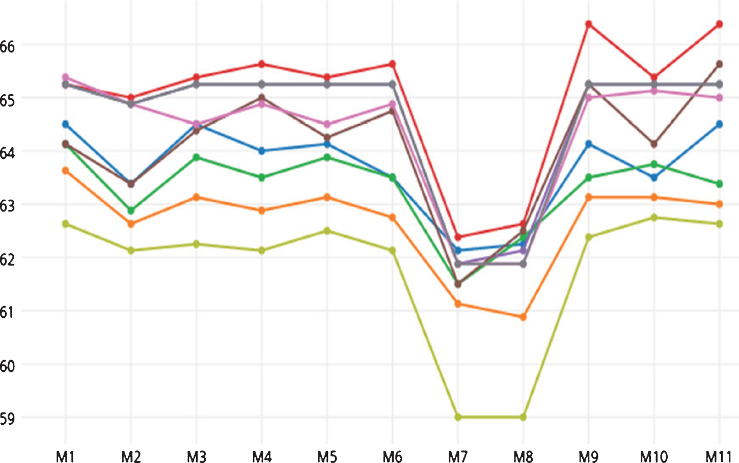
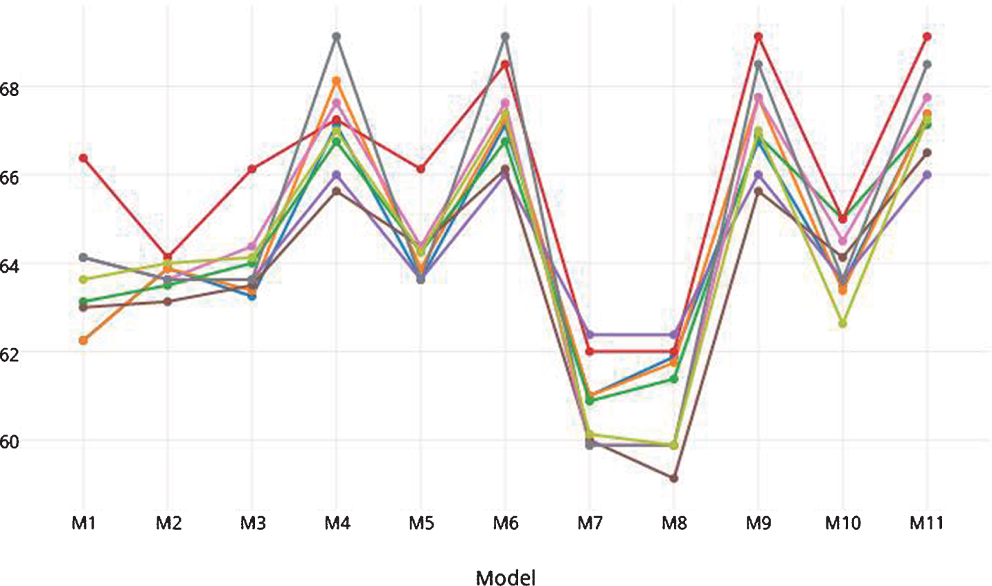
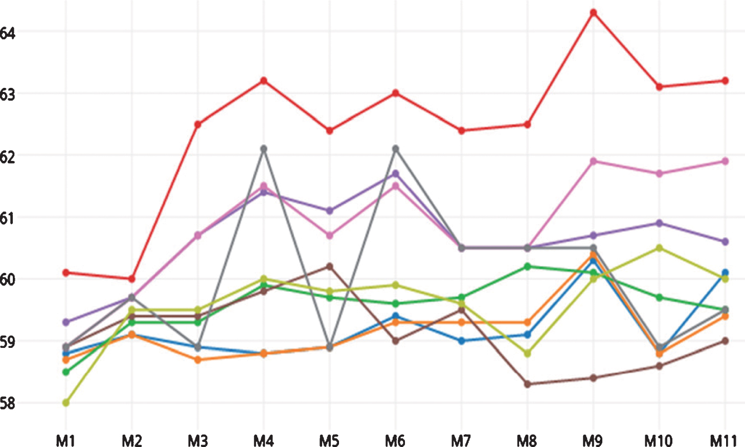
Figures 2 5 show the performance of the classifiers with our models on RTE1 to RTE4 testsets. For all datasets, the LogitBoost classifier exhibits the best performance attaining 61.88%, 66.38%, 69.13% and 64.3% accuracy for RTE1 to RTE4 datasets, respectively. For the RTE3 testset (Fig. 4), the J48 classifier also attains the best accuracy along with LogitBoost.

Fig.2

Accuracy on RTE1 testset.

Fig.3

Accuracy on RTE2 testset.

Fig.4

Accuracy on RTE3 testset.

Fig.5

Accuracy on RTE4 testset.

Model-wise performance shows the role of different combinations of our seven features. Among these, F1 and F2 serve as the baseline ones. Since model M11 combines all features, all of which we deem as important in making entailment decision, one would hope that it should achieve the best performance. However, Fig. 6 shows that with some classifiers M9 performs slightly better than M11.

Fig.6

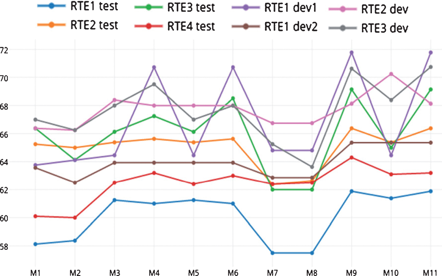
Model-wise performance evaluation using LogitBoost algorithm.

The role of F3 (named entity-matched ratio) is seen by comparing the model pairs M3– M4, M5– M6, and M9– M10 on different datasets and classifiers. The role of F4 (antonym bit), F5 (negation bit), and F6 (superlative degree modifier bit) is seen by comparing the pairs M3– M5, M4– M6, M7– M8 and M9– M11. The role of F7 (entailment score) is seen from the pairs M3– M10, M4– M9, and M6– M11.

From Fig. 2, comparing the performance of the model pairs M3– M4 (for Logistic, Simple Logistic, Multilayer Perceptron, and NaiveBayes) and M9– M11 (for Logistic, Simple Logistic, SMO, and LogitBoost) indicate that the feature F3 is useful in improveing the accuracy. Slight improvements in the model pairs M3– M5 (for Simple Logistic, SMO, Multilayer Perceptron), M4– M6 (for Simple Logistic, SMO, Multilayer Perceptron), M7– M8 (for SMO, Multilayer Perceptron, J48) and M9– M11 (for Simple Logistic, SMO, Multilayer Perceptron, J48, Naivebayes) show that F4, F5, and F6 are important.

The role of F7 is seen from the model pairs M3– M10 (for Logistic, Simple Logistic, SMO, LogitBoost, Multilayer Perceptron, and NaiveBayes), M4– M9 (Logistic, SMO, LogitBoost) and M6– M11 (Logistic, Simple Logistic, SMO, LogitBoost, Multilayer Perceptron, J48). The model pairs M3– M4 (for the curves of LogitBoost, Multilayer Perceptron, BayesNet) and M9– M10 (for Logistic, LogitBoost, Multilayer Perceptron) in Fig. 3 show the role of F3.

The model pairs M3– M5 (NaiveBayes), M7– M8 (for Logistic, SMO, LogitBoost, AdaBoost, Multilayer Perceptron) and M9– M11 (for Logistic, Multilayer Perceptron, NaiveBayes) show the role of F4, F5, and F6. The role of feature F7 is seen from the model pairs M3– M10 (for BayesNet, NaiveBayes), M4– M9 (for Logistic, Simple Logistic, LogitBoost, Multilayer Perceptron, BayesNet, NaiveBayes) and M6– M11 (for Logistic, Simple Logistic, LogitBoost, Multilayer Perceptron, BayesNet, NaiveBayes).

The curves in Fig. 4 reveal the importance of feature F3 on comparing the performance of the model pairs M3– M4 (for Logistic, Simple Logistic, SMO, LogitBoost, AdaBoost, Multilayer Perceptron, BayesNet, J48, NaiveBayes) and M9– M10 (for Logistic, Simple Logistic, SMO, LogitBoost, AdaBoost, Multilayer Perceptron, BayesNet, J48, NaiveBayes).

The role of the features F4, F5 and F6 is seen from the performance of the model pairs M3– M5 (for Logistic, Simple Logistic, SMO, Multilayer Perceptron, NaiveBayes), M4– M6 (for LogitBoost, Multilayer Perceptron, NaiveBayes), M7– M8 (for Logistic, Simple Logistic, SMO) and M9– M11 (for Logistic, SMO, Multilayer Perceptron, NaiveBayes).

The improvement of accuracy for the feature F7 can be seen by comparing the model pairs M3– M10 (for Logistic, SMO, Multilayer Perceptron, BayesNet), M4– M9 (for LogitBoost, BayesNet) and M6– M11 (for Logistic, Simple Logistic, SMO, LogitBoost, Multilayer Perceptron, BayesNet).

By observing the difference between the model pairs M3– M4 (for the curves of Simple Logistic, SMO, LogitBoost, AdaBoost, Multilayer Perceptron, BayesNet, J48, NaiveBayes) and M9– M10 (for Logistic, Simple Logistic, SMO, LogitBoost, BayesNet, J48) in Fig. 5, the role of feature F3 is seen.

The importance of F4, F5, and F6 is seen from the model pairs M3– M5 (for Simple Logistic, SMO, AdaBoost, Multilayer Perceptron, NaiveBayes), M4– M6 (Logistic, Simple Logistic, AdaBoost), M7– M8 (Logistic, SMO, LogitBoost) and M9– M11 (Multilayer Perceptron). The positive role of F7 is seen from the pairs M3– M10 (for Simple Logistic, SMO, LogitBoost, AdaBoost, BayesNet, NaiveBayes), M4– M9 (Logistic, Simple Logistic, SMO, LogitBoost, BayesNet), and M6– M11 (Logistic, Simple Logistic, LogitBoost, BayesNet, NaiveBayes).

Since the LogitBoost algorithm shows the best performance for all datasets of RTE1 to RTE4, Table 14 summarizes the results obtained from the 11 models with this particular algorithm only. Experiments were carried out separately on two devsets and testset of RTE1, devset and testset of RTE2, devset and testset of RTE3 and testset of RTE4. The table shows that in addition to model M11 (which is the combination of all the features) the accuracy of the method (for some datasets) reaches its peak value for the models M9 and M10 also. Figure 6 shows the variation of the performance of the method for the eleven models using LogitBoost classifier.

Table 14

Accuracy (%) of the method for various RTE datasets using different models by LogitBoost Algorithm

Model	RTE1			RTE2		RTE3		RTE4
	dev1	dev2	test	dev	test	dev	test	test
M1	63.76	63.57	58.13	66.38	65.25	67.00	66.38	60.10
M2	64.12	62.5	58.38	66.25	65.00	66.25	64.13	60.00
M3	64.46	63.93	61.25	68.38	65.38	68.00	66.13	62.50
M4	70.73	63.93	61.00	68.00	65.63	69.50	67.25	63.20
M5	64.46	63.93	61.25	68.00	65.38	67.00	66.13	62.40
M6	70.73	63.93	61.00	68.00	65.63	68.00	68.50	63.00
M7	64.81	62.86	57.50	66.75	62.38	65.25	62.00	62.40
M8	64.81	62.86	57.50	66.75	62.63	63.63	62.00	62.50
M9	71.78	65.36	61.88	68.13	66.38	70.63	69.13	64.30
M10	64.46	65.36	61.38	70.25	65.38	68.38	65.00	63.10
M11	71.78	65.36	61.88	68.13	66.38	70.75	69.13	63.20

Table 15 compares the accuracy of our hybrid ML method with the rule-based method presented in [26]. Our method outperforms the rule-based one by a good margin and has better rank with respect to the systems submitted to PASCAL RTE challenges.

Table 15

Comparison of our ML-based method with the rule-based method

Dataset	Accuracy (%)		Rank w.r.t RTE submissions
	Our ML	Rules	Our ML	Rules
RTE1	61.88	60.5	2	3
RTE2	66.38	64.5	3	3
RTE3	69.13	62.8	4	20
RTE4	64.3	61.5	7	8

Comparison of our method with those submitted to the RTE challenges show that out of 28, 41, 45 and 45 submitted systems in RTE1 [28], RTE2 [29], RTE3 [30], and RTE4 [31] challenges, respectively, only 1, 2, 3 and 6 systems are ahead of us in terms of accuracy, which clearly indicates that the proposed method is quite competent with respect to the state of the art methods reported in the literature so far.

6 Error analysis

Our method can give wrong results for the following reasons: errors in datasets, wrong functioning of the embedded tools, and limitations of our method.

Errors in datasets. There are typos in many T– H pairs in the RTE datasets. This causes the tools embedded in this work to produce wrong outputs leading to diminish the ultimate accuracy of the method. Since these are standard datasets, for fair comparison in our experiments we avoided any text normalizing to correct those erroneous phrases. Though such typos reduced the accuracy of the method, this is not a drawback of the method itself.

Errors of the embedded tools. We used a number of NLP tools and resources, such as Stanford dependency parser1, Stanford stemmer2, Stanford Named Entity Recognizer3, WordNet 2.1, WordNet:: Similarity package4, and WEKA. Any errors of these tools reduce the accuracy of the method. E.g., consider a T– H pair from RTE2 devset:

Example 9. T: American illusionist, James Randi, offered $1m to anyone able to prove, under observed conditions in a laboratory, that homeopathic remedies can really cure people. H: Illusionist James Randi offered a million dollars to anyone able to prove that homeopathy cures.

Table 16 presents some dependency triples produced by the Stanford parser for the T– H pair from Example 9 with wrong triples, shown in bold, caused by errors of the Stanford POS tagger, which propagate to parsing. The wrong POS-tagged output of the Stanford POS tagger is shown in Table 16 highlighted in bold. These erroneous hypothesis dependency triples H1 and H2 do not satisfy any of the matching criteria in [26] to find a match with any of the text triples thus producing low scores for the features F1, F2, and F7. Therefore, the accuracy of our method was limited by correctness of the embedded tools.

Table 16
Generated incorrect dependency triples by Stanford parser for T– H pair of Example 9

T dependency triples H dependency triples POS-tagged H tokens

T1: amod(remedies-25, homeopathic-24) H1: amod(cures-15,homeopathy-14) cures-NNS

T2: nsubj(cure-28, remedies-25) H2: dobj(prove-12,cures-15) prove-VB

T dependency triples	H dependency triples	POS-tagged H tokens
T1: amod(remedies-25, homeopathic-24)	H1: amod(cures-15,homeopathy-14)	cures-NNS
T2: nsubj(cure-28, remedies-25)	H2: dobj(prove-12,cures-15)	prove-VB

Moreover, the lexical database WordNet 2.1, which we used as the underlying knowledge base, does not provide sufficient coverage of antonymy relation. For the T– H pair from Example 10, the highlighted tokens dip and rise are antonyms, but due to insufficient coverage of antonyms in WordNet 2.1 they cannot be lexically aligned to each other. This prevents the feature variables F1, F2 and F7 from being assigned low values, and the feature F4 (Antonym bit) cannot be set to 1:

Example 10. T: Crude oil dips below $43 on news that Russia’s justice ministry will not force Yukos to halt sales. H: Crude oil rises.

Limitations of the method. The erroneous output produced by the method can be of two types: false positives and false negatives. The reason behind generating such outputs is explained with two T– H pairs provided in Examples 11 and 12, respectively.

Example 11. A male rabbit is called a buck and a female rabbit is called a doe, just like deer. A female rabbit is called a buck.

Example 12. The wait time for a green card has risen from 21 months to 33 months in those same regions. It takes longer to get green card.

In the T– H pair of Example 11, each dependency triple of H finds a corresponding match with some text triples leading to generation of high scores for F1, F2 and F7. The high values of the feature variables eventually restrict the ML-based classifiers to mark the given T– H pair as a case of no entailment.

On the other hand, although a human reading of the hypothesis of the T– H pair in Example 12 infers the truth of the text, it is difficult to be captured by this method. Since the hypothesis conveys the same information as that of the text but in a completely different way, no dependency triples of H find their matching counterpart in the T triples thereby generating very low scores at the feature variables F1, F2 and F7 ultimately leading to incorrectly classifying the given T– H pair as a case of no entailment.

7 Conclusion

We have presented a hybrid approach for recognizing textual entailment, which blends a rule-based method for feature extraction with supervised ML-based framework for decision-making. A set of as few as seven features was extracted using matching rules that mainly compare syntactic structures of lexically aligned tokens, as well as semantic similarity between a pair of non-lexically aligned tokens.

We carried out exhaustive experiments on different combinations of those features using several ML-based classifiers, of which LogitBoost showed the best performance. Our results show that our hybrid approach efficiently labels a good percentage of T– H pairs as textually entailed or not. The technique, being a combination of rule-based and ML-based method, outperforms many systems reported so far. Although our method still does not outperform the best known methods, it is much lighter in terms of tools and resources used, thus being suitable for implementation for low-resource languages.

In the future, we will explore other features in order to increase the accuracy of the method.

Footnotes

Acknowledgments

S.K. Naskar is supported by Media Lab Asia, Meit Y, Government of India, under the Young Faculty Research Fellowship of the Visvesvaraya PhD Scheme for Electronics & IT. A. Gelbukh was supported by the SNI, Mexico, and Instituto Politécnico Nacional grants SIP 20172008 and SIP 20172044.

References

Pakray

, Bandyopadhyay

and Gelbukh

, Answer Validation using Textual Entailment, Proc International Conference on Intelligent Text Processing and Computational Linguistics, CICLing 2011 Lecture Notes in Computer Science 6609 (2011);359–364.Springer.

Pakray

, Gelbukh

and Bandyopadhyay

, A Syntactic Textual Entailment System Based on Dependency Parser, Proc International Conference on Intelligent Text Processing and Computational Linguistics, CICLing 2010 Lecture Notes in Computer Science 6008 (2010), 269–278.

Rios

, Specia

, Gelbukh

and Mitkov

, Statistical Relational Learning to Recognise Textual Entailment, Proc International Conference on Intelligent Text Processing and Computational Linguistics, CICLing 2014 Lecture Notes in Computer Science 8403 (2014).330–339.Springer.

Akhmatova

, Textual Entailment Resolution via Atomic Propositions, Proc of the First PASCAL Recognizing Textual Entailment Workshop.2015.

Pakray

, Poria

, Bandyopadhyay

and Gelbukh

, semantic textual entailment recognition using UNL, Polibits43 (2011), 23–27.

Rios

and Gelbukh

, Recognizing textual entailment with a semantic edit distance metric IEEE, 11th Mexican International Conference on Artificial Intelligence (MICAI 2012) (2012).15–20.

Kouylekov

and Magnini

, Recognizing textual entailment with tree edit distance algorithms, Proc of First Workshop Recognising Textual Entailment (2005), 17–20.

Marsi

E.C.

, Krahmer

E.J.

, Bosma

W.E.

and Theune

, Normalized alignment of dependency trees for detecting textual entailment, 2006.

Herrera

, Penas

and Verdejo

, Textual entailment recognition based on dependency analysis and wordnet, Machine Learning Challenges, Evaluating Predictive Uncertainty, Visual Object Classification, and Recognising Textual Entailment (2006), 231–239.Springer.

10.

Blake

, The role of sentence structure in recognizing textual entailment, pp, Proc of ACL-PASCAL Workshop on Textual Entailment and Paraphrasing, ACL (2007), 101–106.

11.

Pakray

, Bandyopadhyay

and Gelbukh

, Dependency parser based textual entailment system IEEE, International Conference on Artificial Intelligence and Computational Intelligence (AICI). 1, (2010).393–397.

12.

Pakray

, Neogi

, Bhaskar

, Poria

, Bandyopadhyay

and Gelbukh

, A Textual Entailment System using Anaphora Resolution, NIST, Proc of TAC 2011, 2011.

13.

Pakray

, Pal

, Poria

, Bandyopadhyay

and Gelbukh

, JU_CSE_TAC: Textual Entailment Recognition System at TAC RTE-6, NIST, Proc of TAC 2010.2010.

14.

Dinu

and Wang

, Inference Rules and their Application to Recognizing Textual Entailment, Association for Computational Linguistics (2009), 211–219.

15.

Malakasiotis

and Androutsopoulos

, Learning Textual Entailment using SVMs and String Similarity Measures, Association for Computational Linguistics (2007), 42–47.

16.

MacCartney

, Grenager

, Marneffe

M.-C.

, Cer

and Manning

C.D.

, Learning to recognize features of valid textual entailments, Proc of HLT-NAACL, ACL (2006), 41–48.

17.

Szpektor

and Dagan

, Learning Entailment Rules for Unary Templates, pp, Proc of the 22nd International Conference on Computational Linguistics (Coling) (2008), 849–856.

18.

Mirkin

, Dagan

and Geffet

, Integrating pattern-based and distributional similarity methods for lexical entailment acquisition, ACL (2006), 579–586.

19.

, Irwin

, Garcia

E.V.

and Ram

, Machine Learning Based antic Inference: Experiments and Observations at RTE-3, 45 Annual Meeting of the ACL (ACL’07), Workshop on Textual Entailment and Paraphrasing (WTEP-2007)–Sem.

20.

Pham

Q.N.M.

, Nguyen

L.M.

and Shimazu

, A Machine Learning based Textual Entailment Recognition System of JAIST Team for NTCIR9 RITE, Japan, Proceedings of NTCIR-9 Workshop Meeting.2011.Tokyo, Japan.

21.

Zanzotto

F.M.

, Pennacchiotti

and Moschitti

, A machine learning approach to textual entailment recognition, Natural Language Engineering15(4) (2009).551–582.doi:.Cambridge University Press.

22.

Agichtein

, Askew

and Liu

, Combining Lexical, Syntactic, and antic Evidence for Textual Entailment Classification, TAC, NIST, 2008–Sem.

23.

Saikh

, Naskar

S.K.

, Giri

and Bandyopadhyay

, Textual Entailment Using Different Similarity Metrics, CICLing 2015, Part I, Lecture Notes in Computer Science, 9041, 491–501. doi:10.1007/978-3-319-18111-0_37

24.

Rios

M.A.

, Gelbukh

and Bandyopadhyay

, Recognizing Textual Entailment Using a Machine Learning Approach. MICAI Lecture Notes in Artificial Intelligence, (2010), 177–185.Springer.

25.

Castillo

J.J.

, An approach to Recognizing Textual Entailment and TE Search Task using SVM, SEPLN, (2010).

26.

Basak

, Naskar

S.K.

and Gelbukh

, A Lexico-Syntactic-semantic Approach to Recognizing Textual Entailment. Submitted;.https://goo.gl/KsbHRs.

27.

Basak

, Naskar

S.K.

, Pakray

and Gelbukh

, Recognizing textual entailment by soft dependency tree matching, Computación y Sistemas19(4), 685–700. 2015. DOI: 10.13053/CyS-19-4-2331

28.

Dagan

, Glickman

and Magnini

, The PASCAL recognising textual entailment challenge, In Machine learning challenges. Evaluating predictive uncertainty, visual object classification, and recognising textual entailment, (2006), 177–190.Springer.

29.

Haim

R.B.

, Dagan

, Dolan

, Ferro

, Giampiccolo

, Magnini

and Szpektor

, The Second PASCAL Recognising Textual Entailment challenge, 2006.

30.

Giampiccolo

, Magnini

, Dagan

and Dolan

, The Third PASCAL Recognizing Textual Entailment challenge, ACL, pp, Proc of the ACL-PASCAL Workshop on Textual Entailment and Paraphrasing (2007), 1–9.

31.

Giampiccolo

, Dang

H.T.

, Magnini

, Dagan

, Cabrio

and Dolan

, The Fourth PASCAL Recognizing Textual Entailment Challenge, TAC, 2008.

A simple hybrid approach to recognizing textual entailment

Abstract

Keywords

1 Introduction

2 Related work

3 Outline of the method

3.1 Pre-processing

3.2 Feature extraction and classification

Table 1 Features used in our experiments Feature Name F1 Sum of in_degree of vertices of H dependency graph F2 Sum of out_degree of vertices of H dependency graph F3 Named entity matched ratio F4 Antonym bit F5 Negation bit F6 Superlative degree modifier bit F7 Entailment score

4.3 Antonym bit (F4)

5 Experiments and results

Table 13 Different models combining several features Model Features Difference 1 2 3 4 5 6 7 M1 + M2 + M3 + + M1 + F2 = M2 + F1 M4 + + + M3 + F3 M5 + + + + + M6 + + + + + + M5 + F3 M7 + M8 + + + + M9 + + + + M10 + F3 M10 + + + M11 + + + + + + + M6 + F7

Footnotes

Acknowledgments

References

Table 1
Features used in our experiments

Feature Name

F1 Sum of in_degree of vertices of H dependency graph

F2 Sum of out_degree of vertices of H dependency graph

F3 Named entity matched ratio

F4 Antonym bit

F5 Negation bit

F6 Superlative degree modifier bit

F7 Entailment score

Table 13
Different models combining several features

Model Features Difference

1 2 3 4 5 6 7

M1 +

M2 +

M3 + + M1 + F2 = M2 + F1

M4 + + + M3 + F3

M5 + + + + +

M6 + + + + + + M5 + F3

M7 +

M8 + + + +

M9 + + + + M10 + F3

M10 + + +

M11 + + + + + + + M6 + F7