
Abstract
In this paper we measure the relationship between messages in the social media and the stock market prices. First, we measure the correlation and association between the amount of stock related tweets and different financial indicators such as prices, returns and transaction volume. Then, we analyze the content of the messages and test whether the tweets generated during different trends of price change (up, down or steady) can be distinguished by automatic classifiers. Our corpus consist on messages related to nine IT companies and also their daily prices and volume during trading hours for over a period of three months. Two textual representations were used, bag of words and word embeddings. The tweets were automatically tagged using two thresholds to bin the changes in price. We have found a correlation between the amount of daily messages and the volume of financial transactions. We also found negative association (more specifically, what we define as local trend association) between tweet volume and financial indicators that were not found by using only the correlation analysis. Our main contribution is that the messages generated during a positive, negative and neutral trend can be distinguished by state of the art classifiers.
Introduction
With the advances in natural language processing and machine learning techniques the task of forecasting the stock market using textual information has grown popularity as more data becomes available. The first works [14, 43] used news as a source of information with promising results . On recent years the works [4, 45] use the social media provided its growth in popularity. Social media embeds not only news but also stock market events, opinions and insights from investors.
We collected Twitter data to create a corpus of messages related to nine IT companies. We choose Twitter because it is a popular platform and also because the messages or tweets are tagged with the company’s stock symbol by the users themselves.
In this study we analyze the tweets generated during different trends, our hypothesis is that it is possible to identify tweets depending on the positive, negative or neutral market trends. We used two different text representations, Bag of Words (BOW) and Word Embeddings (WE), for the latter word2vec, a model trained on news, is used. Previous works compare textual representations in the task of sentiment analysis using a manually tagged set, however we tag a tweet automatically by the trend in which it appeared. Our results are contrasted against a baseline that considers the distribution of the corpus. Not many related works consider how the distribution of the data may influence the results [22].
We also study whether tweet volume is correlated with the transaction volume or returns indicators and whether it can be helpful on the task of forecasting. We consider also negative relationships using a measure of local trend association [2]. Previous studies do not consider the trading hours, which are important since after the market closes new topics are generated that may not be related with the previous price but with next day’s price.
The rest of the paper is structured as follows. In Section 2, we present the related works. In Section 3, we describe the corpus. In Sections 3.1 and 3.2, we present experiments with tweet volume and in Section 3.3, experiments with the content of the tweets. Section 4 includes conclusions and future work.
Related work
There are two main paradigms in forecasting the stock market: technical [18] and fundamental [1] analysis. The first approach analyzes the historical prices of the time series themselves using methods such as auto-regression, ARIMA, state-space models, neural networks and others. The second approach relies on financial indicators such as the overall economy, unemployment, welfare indicators, etc.
There have been numerous approaches to integrate automatically other information than in fundamental or technical analysis in the stock market prediction.
One of the first research works that investigates such strategies is done by Sankaran [36]. In his work, traders are asked to assign weights to different attributes they call “unmeasurable factors”, including government policies or political news that may influence the exchange rates. In this approach the knowledge of experts is taken from the news they read and other internal information they posses, but the news are not directly processed.
Leung [17] creates a system that requests the user to manually download news before the market opens to predict the Hang Seng Index, generating decision rules from the news articles. Later, in [43], Leung’s approach is extended by adding other global indexes such as DJIA and FTSE and improving the processing techniques. This last approach resulted in greater performance forecasting the DJIA, it was attributed to the fact that most news sources they used were from the U.S.
Lavrenko et al. [14] collect news automatically, they consider prediction as a classification problem. The text from the news is aligned with the future financial time series trend. He analyzed different companies, one of his interesting findings is that the same word may have different effects for different companies. The set up of prediction as a classification problem has been widely used in the literature [11, 47].
Lee et al. [16] create a corpus of financial reports that ranges form 2002 to 2012. They tested several machine learning methods, the method reported with the best results was Random Forest. In this article financial and text features are combined, both extracted from the reports. Twenty one financial features are used, the most helpful being the earnings surprise (the difference between expected and reported earnings for a given company). It was found that adding text features to financial features improved the accuracy from 50.1 to 55.5.
In Zhang’s dissertation [47] the corpus from [16] was used. He implemented three different neural networks architectures. Although they did not considered the financial features but only language features the accuracy he reported was better than Random Forest and Support Vector Machine classifiers. He selected only 15 from the 1500 companies in the corpus.
On recent years it is common to use information from social media, considering that it is a channel for communication changing the ways users interact with the news [15]. Social media includes information from different sources. In [13] it was found that 85% of the topics in social media are related to news.
Twitter is a micro-blogging social media platform launched in 2006. Its mission is “To give everyone the power to create and share ideas and information instantly, without barriers”. It has 313 million active users1 and any topic can be tackled in this platform including discussions related to the stock market. When a company stock is being discussed it is clearly referenced by preceding its stock symbol with the dollar sign e.g. $MSFT stands for the Microsoft’s stock symbol.
Some of the advantages of twitter are the inclusion of different sources of information and the summarization of this information, since only messages shorter than 140 characters are permitted. One of the disadvantages is that we can find noisy tweets in the form of adds or fake news. Wolfram [42] points out that his results could have been improved handling better the noise. Zhang et al. [46] only consider re-tweets with the rationale that if it is re-tweeted then it is more relevant to users.
Social media can be explored in different manners. De Choudhury et al. [8] correlate the magnitude of individual stocks’s price change with features of user interaction such as the number of comments on a post, the numbers of replies to them, the elapsed time between each comment and other several features. Another interesting approach by Ruiz et al. [35] is the representation of social media as a graph and the analysis of correlations between the features of the graph and the price and volume of company stocks. An interesting challenge in processing social media data is tackling multimodal information, which is the subject of the research field of multimodal sentiment analysis [6, 44].
A popular approach to forecast the stock market is the use if sentiment analysis techniques. This is usually done for predicting large indicators such as DJIA or S&P [4, 45], but it is also used for the stocks of individual companies [7, 38].
Tetlock [40] uses a psychosocial dictionary, the General Inquirer’s Harvard IV-4, to measure the sentiment of a Wall Street column. It was found out that pessimism causes downward trends and that either high or low pessimism can predict high trading volume. Bollen et al. [4] predicted the daily up and down changes in the closing values of the DJIA using different mood indicators such as happy, alert or calm.
The results of forecasting using sentiment analysis at company level are different from those at market level. Oliveira et al. [23] did not find predictive power for the returns even after trying with five different sentiment lexicons, nor did they find a significance difference among the lexicons. De Fortuny et al. [9], also at company level, compare BOW against sentiment analysis, they found out that the latter performed worse than the former and even worse than random. They attribute this behavior to the fact that sentiment lexicons are usually extracted from different contexts, such as book or movie reviews. Even more, in finance sometimes the nouns and verbs are more informative for decision making than the adjectives. Lee et al. [16], predicting individual company stocks, used generic and specialized sentiment lexicons, none of such approaches boosted the accuracy results.
From the evidence in the literature it seems that sentiment analysis is more useful at the global market level than at the company stocks level.
Besides returns, the transaction volume is another variable than has been studied, it can be defined as the number of transactions performed in a given period of time. Transaction volume is useful to study because in technical analysis it determines the importance of the changes in price and the risk involved in a transaction.
Ruiz et al. [35] tested correlation at different lags between volume and graph features generated from Twitter interaction. The greatest correlation was found at lag zero. Mao et al. [20] found weak correlation between price and tweets mentioning the stock symbol AAPL, and moderate correlation to the daily volume traded. Sprenger et al. [39] and Oliveira et al. [23] found that the message volume is useful to predict the next-day trading volume using regression analysis.
Experimental setup
The tweets were collected from March 23, 2017 to July 3, 2017 using the Twitter API tweepy [34]. We only considered tweets with a single company in the message, this operation reduced the corpus up to 25% of its original size. The rationale for this filter was the observation that tweets with more than one stock symbol mentioned were either advertisements or contained a relationship between such entities that is outside of our scope. By filtering out such tweets it is also avoided to use the same tweet for different forecasts. A total of 141’007 tweets were used in the analysis. The stock symbols chosen based on their popularity are amzn (Amazon.com, Inc.), aapl (Apple Inc.), fb (Facebook Inc.), goog (Alphabet Inc.), msft (Microsoft Corporation), snap (Snap Inc.), twtr (Twitter Inc.), yhoo (Yahoo Inc.)2 and znga (Zynga Inc.). Other stock symbols were considered but not enough tweets were collected (less than 100). The distribution of the tweets3 in the corpus is shown on Fig. 1. The average of daily tweets is shown in Table 1. Below we show a sample of the tweets.
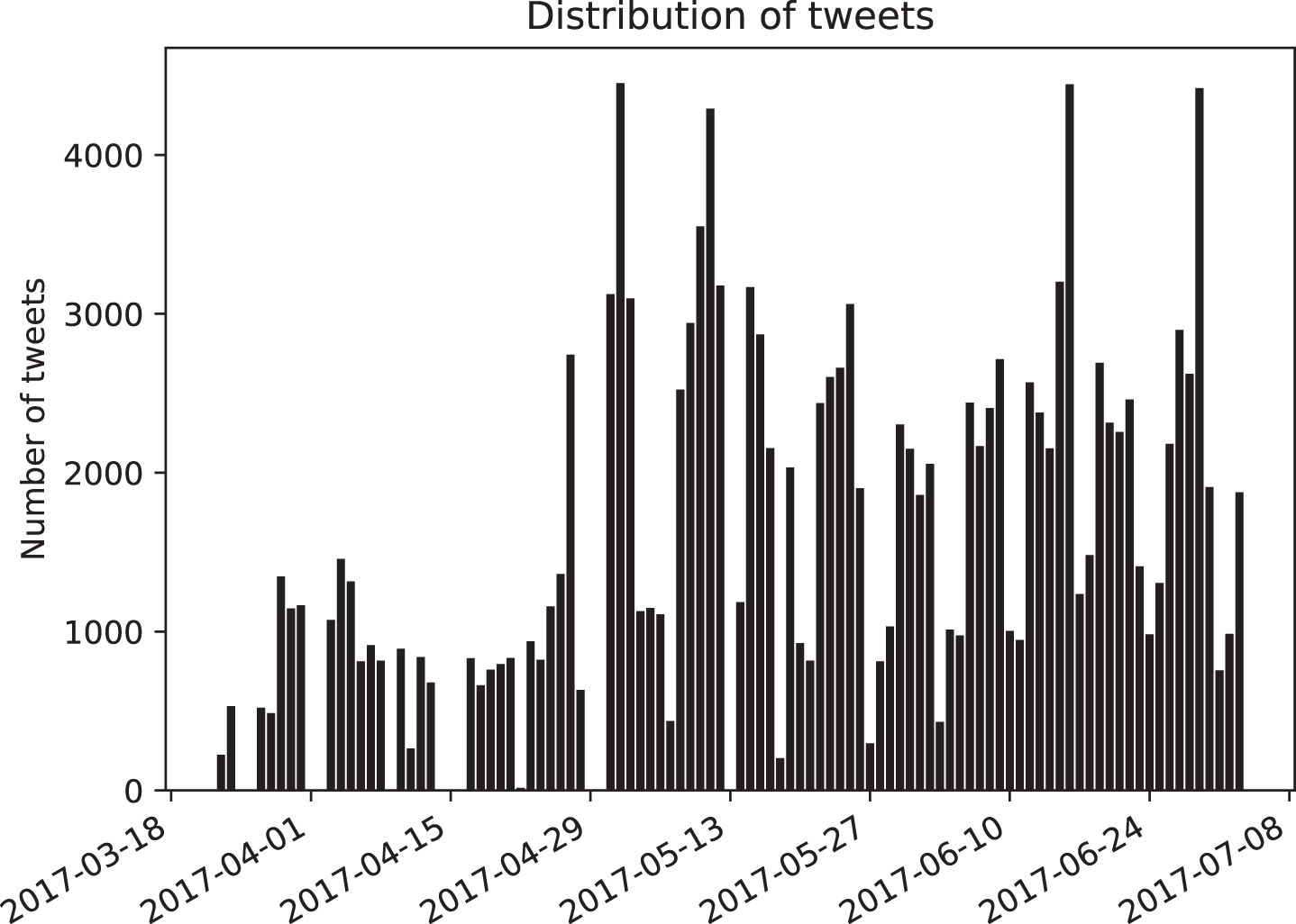
Distribution of tweets through the corpus.
Average of daily tweets per company
“$AMZN Amazon launches store-pick grocery service in Seattle <url> ”
“Signal is Positive upward for Apple! $AAPL #AAPL #stocks #DayTrade #AI”
“#Facebook Messenger Reaches 1.2B Monthly Active Users Milestone. Read more: <url> $FB”
“Insider Trading Activity Alphabet Inc (NASDAQ:GOOG) Director Sold 24 shares of Stock <url> $GOOG”
The daily stock prices at open and close market times and the volume were collected from Google Finance.4
BOW is a traditional approach that has been widely used in the literature, it is a subclass of n-gram representation in which a word represents one dimension in a document vector. A word is represented by the number of times that it appeared in the document.
Word embeddings is the representation of words as vectors, it is a recently proposed methodology by Mikolov [21]. We used the Word2Vec vectors5 obtained from a trained distributed representation on news with three million words, each word is represented by a 300-dimensional array. The semantics captured by this model allows operations among words, a popular example of such powerful operation of the trained model is: “king” - “man” + “woman” = “queen”.
It was tested a lagged correlation between the daily number of tweets per company against the company’s open price, close price, the difference between close and open prices, the absolute value of such difference, transaction volume, returns
The time series of the tweets is created with the days for which at least one tweet was collected. The days with zero tweets are not considered as point in the correlation even if it is a working day, this is because not for all companies we started downloading at the same time.
In Table 2 we show the results for |ρ|>0.5, where ρ is the Pearson’s correlation coefficient. Although we compared with all the indicators mentioned above volume was the indicator that appeared the most. The column Days indicates the total number of points of the time series, for each lag a point is lost. High correlation with a lag 1 indicates that the number of tweets may cause the price or transaction volume fluctuation of the next day. High correlation with lag -1 indicates that the price or transaction volume may cause the next day’s tweet volume.
Higher results for lagged correlation between tweet volume and financial indicators using a lag from -3 to 3
The time series shown on the Figs. 1 and 2 are z-normalized using
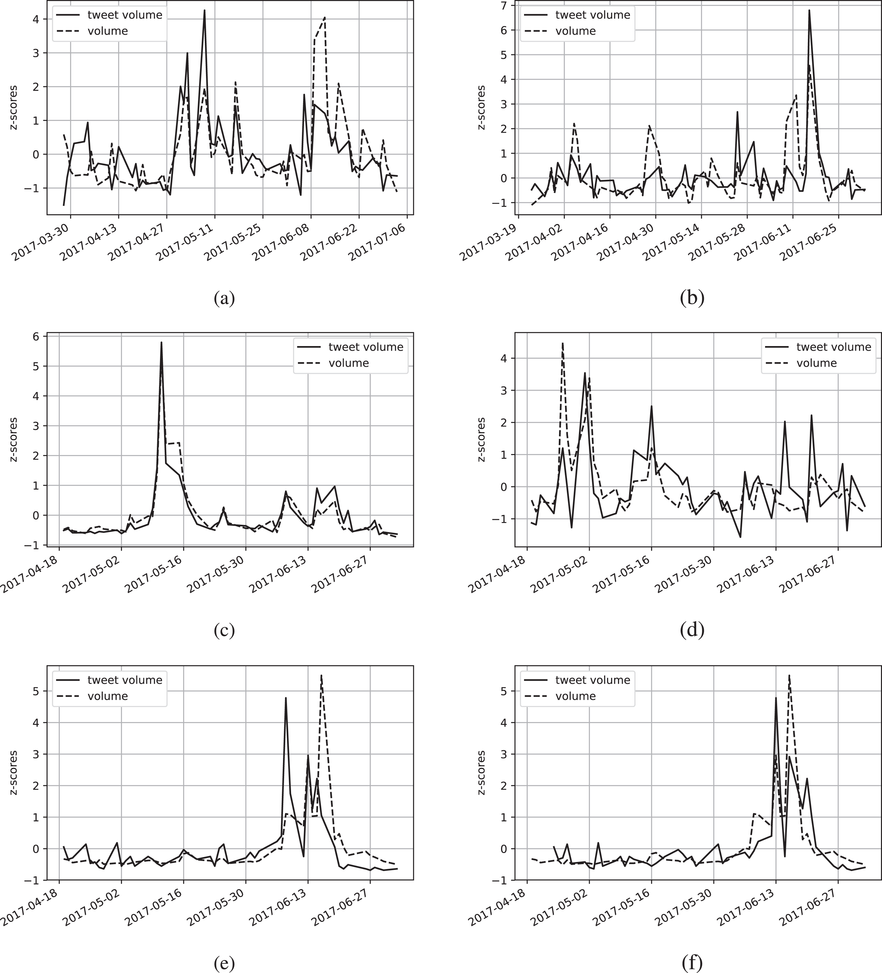
(a) Correlation between Apple’s tweet volume and transaction volume lag = 0, ρ = 0.61; (b) Correlation between Amazon’s tweet volume and transaction volume lag = 0, ρ = 0.64; (c) Correlation between Snapchat’s tweet volume and transaction volume lag = 0, ρ = 0.96; (d) Correlation between Twitter’s tweet volume and transaction volume lag = 0, ρ = 0.51; (e) Correlation between Yahoo’s tweet volume and transaction volume lag = 0, ρ = 0.60; (f) Correlation between Yahoo’s tweet volume and transaction volume lag = 3, ρ = 0.77. For Figures
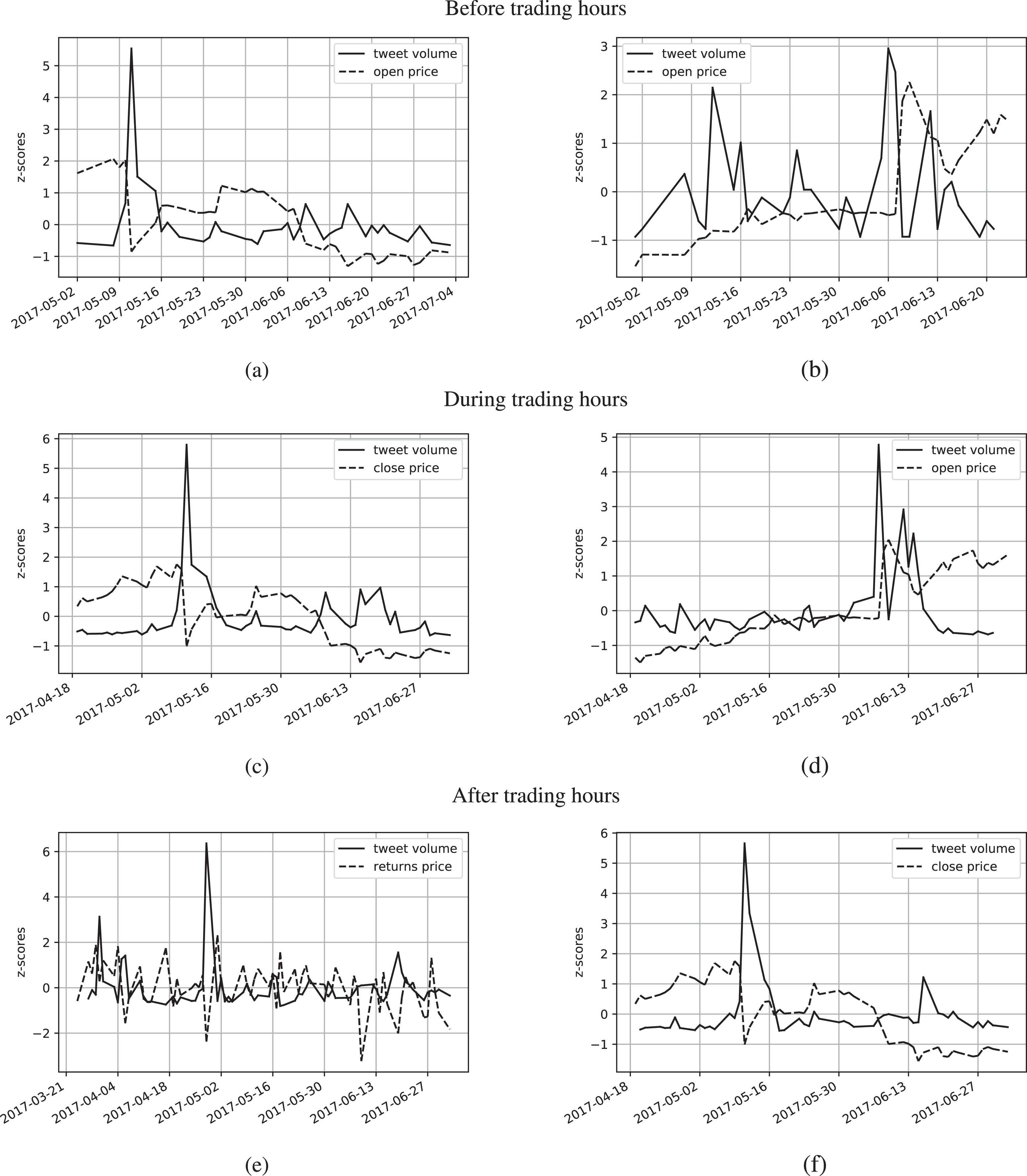
Associations between (a) Snapchat’s tweet volume and open price lag = 0, ρ = -0.17, LTAM = -0.74; (b) Yahoo’s tweet volume and open price lag = -2, ρ = -0.22, LTAM = -0.58; (c) Snapchat’s tweet volume and close price lag = 0, ρ = -0.19, LTAM = -0.61; (d) Yahoo’s tweet volume and open price lag = -1, ρ = 0.14, LTAM = -0.57; (e) Amazon’s tweet volume and returns lag = 1, ρ = -0.34, LTAM = -0.55; (f) Snapchat’s tweet volume and close price lag = 1, ρ = -0.19, LTAM = -0.75. For Figures
We can observe from Table 2 that tweet volume and trading volume showed more correlation at lag 0. This is consistent with [35], where the greatest correlation on average was ρ = 0.4728 at lag 0 and between tweets and trading volume. However they use the total number of tweets during the day, the daily change in close prices and daily traded volume. We also tried the total number of tweets during the day achieving similar results. Another interesting observation is the case of the company Snapchat, the result indicates that the volume of tweets the night before and the morning before are highly correlated with the transaction volume during the following trading hours.
The Moving Approximation (MAP) transform [2, 3] is the transformation of a time series of size n into a series of n - k + 1 local slopes. In order to obtain the slopes a linear least squares regression is passed through the time series using a sliding window of size k. The Local Trend Association Measure (LTAM) is the measure of cosine similarity between the series of slopes of two time series. The MAP transform and the LTAM use the time series trends instead of point to point comparison as in correlation analysis. The higher results of LTAM are shown on Table 3. Figure 2 depicts some of the associations found.
Higher results for lagged Local Trend Association measure between tweet volume and financial indicators using a lag from -3 to 3
Higher results for lagged Local Trend Association measure between tweet volume and financial indicators using a lag from -3 to 3
Using the LTAM we found negative associations not obtained by the correlation analysis.
The task of tweet classification is done by automatically tagging the tweets according to the price trend in which they were generated, upward, downward or neutral. Then, a machine learning classifier is trained on some portion of the tweets randomly selected to predict the tag of the remaining tweets.
We used two word representations, BOW and WE, and different machine learning classifiers included in the scikit-learn API [5].
Tweet and stock time series are labeled with different time zones. It was necessary to adjust the tweets UTC time-stamp to match financial time series ET time zone. NYSE and NASDAQ markets open at 9:30 ET and close at 16:00 ET.
We used two different thresholds, 0.3 (Leung’s tagging) and 0.5 (Wütrich’s tagging), for an automated binning procedure to tag the tweets in the following manner. If the price change is greater or equal than the threshold then the tweet is considered positive, if the price change falls beyond the threshold the tweet is considered negative, otherwise the tweet is considered neutral. This type of tagging for the prices was used in [17] and [43]. The distrubution of the different tagging schemes is depicted in Table 4.
Tag balance using different offsets
Tag balance using different offsets
We measure price change with Equation 1. For tweets generated within trading hours p t is the close price and pt-1 is the open price of the tweet date. For tweets generated outside trading hours p t is the next open price and pt-1 is the previous close price.
The preprocessing steps are as follows: (a) Lowercase the tweet. (b) Replace links by the word url. (c) Replace usernames by the word username. (d) Remove the stock symbol. (e) Replace some non-ambiguous english contractions e.g. “’m” with “am”. (f) Tokenization. (g) Remove stopwords. (h) Remove tokens that are numbers. (i) Remove tokens that do not contain letters. (j) Remove continuous repeated letters in each token if there are more than three, e.g. “haaaaaappy” is replaced by “happy”.
In the BOW approach we tried with different vocabulary sizes, a size of 1000, with the most common words gave the best results.
In the WE approach each word was transformed to their Word2Vec representation, i.e. a 300-dimensional vector. Tweets in which none of its words were found on the Word2Vec model are discarded. Then all retrieved vectors are averaged to obtain a single 300-dimensional vector that represents the tweet. The process of averaging all words returns a vector that is semantically similar to the tweet vectors [41].
Tweets are split randomly using 70% for train and the rest for test. We tested different classifiers, however the ones with greater accuracy are shown on Tables 5 and 6.
Results for Bag of Words, the baseline is majority vote (MV), the voting classifier (VC) considers the classifiers in the three previous columns
Results for Word Embeddings, the baseline is majority vote (MV), the voting classifier (VC) considers the classifiers in the three previous columns
We used majority vote (MV) as baseline, which consists on predicting always the class with more examples on the training set. We also implemented a voting classifier (VC), which votes among the classifier predictions.
Dickinson [10] and Pagolu [24] compare both word representations on the sentiment classification task of stock tweets, they manually tagged tweets from the time series, 1000 and 3216 tweets respectively. Dickson obtained an accuracy of 68.5% for n-gram model and 63.4% for WE model, Pagolu obtained 70.5% and 70.2%. Comparing with these works, our task is to classify the tweet according to the trend in which they were generated. In our case the W2V approach gave better results than BOW.
We tried different classifiers such as Naive Bayes, k-nearest-neighbors, logistic regression or multilayer perceptron however the top three classifiers were selected based on the accuracy results. Once the best classifiers were selected, their parameters were optimized. The best ones are shown next. The parameters of the BOW classifiers were: For support vector classifier (SVC) RBF kernel, γ = 10 and C = 10. For decision tree (DT) maximum depth of tree = 10. For random forest (RF) Trees = 10, maximum depth of tree = 10. The parameters of the W2V classifiers were: For support vector classifier (SVC) RBF kernel, γ = 2 and C = 1. For stochastic gradient descent classifier (SGD) Default parameters. For random forest (RF) Trees = 10, maximum depth of tree = 5.
Analyzing results from Table 6 we see that the threshold of 0.5 gave better results, this may be because such threshold generates a less balanced set. However using the threshold of 0.3 two out of the three classifiers are also able to learn and surpass the threshold. The amount of data did not play a significant role. The companies YHOO and ZNGA with the less tweets performed better than AMZN or AAPL. Also in the WE approach with Wütrich’s tagging the difference between baseline and SVC for the companies FB (32627 tweets) and YHOO (1777 tweets) is similar.
In Table 5 the accuracy results using the BOW representation mostly fall under the baseline. However in Table 6, using the WE representation, the classifiers are able to surpass the threshold and therefore to identify the tweets during different trends, positive, negative and neutral. For the four tables two different tagging schemes were used.
To test the statistical significance of the accuracy results with respect to baseline we applied the McNemar’s test with
Here, e01 is the number of examples that the baseline classified correctly and our classifier incorrectly and, correspondingly, e10 is the number of examples that our classifier classified correctly and the baseline incorrectly.
McNemar’s test is a measure of the significance between two classifiers considering the examples on the test set where the classifiers disagree. On Table 6 considering Leung’s tagging for the stock TWTR we observe that SGD and the baseline have the same accuracy but the difference is statistically significant. This can be explained because although the same number of sample were classified correctly, the samples were not the same ones. As expected we can see that companies with more tweets showed the higher statistical significance. In Tables 5 and 6 the p-values smaller than 0.01 are marked with ** and p-values smaller than 0.05 are marked with *. The accuracy results greater than the baseline are in bold.
We show that the tweet messages generated during a positive, negative and neutral trends of stock prices can be distinguished by state of the art classifiers. This means that the topics on social media depend on the price change of a company’s stock. We measure our results considering how the balance of the dataset may influence the results.
The results obtained using Word Embeddings representation of tweets significantly outperform the results obtained by Bag of Words. This may be caused by the significant reduction in the dimensionality.
For more than half of the considered companies, we found moderate correlation between tweet volume and trading volume, which is consistent with the findings in [35] and with the Efficient Market Hypothesis [19]. We showed that for two of the companies tweet volume can be used for prediction of transaction volume with lag of one or three days. Regarding the consideration of the trading hours we found for one company that the volume of tweets generated the day before after the close time is correlated with the volume during trading hours the next day.
We also used the MAP transform and the LTAM to find associations between the tweet volume different indicators. We found inverse relationships that were not discovered by correlation analysis. For this reason, LTAM can be used as complementary measure to the correlation coefficient.
As our future work, we will increase the corpus size, try different techniques on the textual representations (e.g. add dimensionality reduction for BOW model) and add semantic analysis of the tweets. We would also combine our text approaches with time series specific forecasting techniques such as regression or ARIMA, this combination has shown good results in the literature [23, 37]. We also aim to use deep learning-based approaches with hierarchical architectures to enhance scalability and increase accuracy of our method [25–29].
Footnotes
On June 19, 2017, Yahoo changed its stock symbol to AABA and although some tweets started to adopt the new symbol, YHOO was still used in Twitter.
There are less tweets at the beginning of the figure because we only considered at first the trading hours. This fact does not affect the experiments since we only consider the days where tweets are available per company.
Acknowledgments
This work was partially funded by CONACYT under the Thematic Networks program (Language Technologies Thematic Network project 281795), as well as by CONACYT Project 283778 and by Instituto Politécnico Nacional grants SIP 20171344, SIP 20172008, and SIP 20172044.