A comparison of fuzzy clustering algorithms for bearing fault diagnosis

Abstract

Bearings are one of the most omnipresent and vulnerable components in rotary machinery such as motors, generators, gearboxes, or wind turbines. The consequences of a bearing fault range from production losses to critical safety issues. To mitigate these consequences condition based maintenance is gaining momentum. This is based on a variety of fault diagnosis techniques where fuzzy clustering plays an important role as it can be used in fault detection, classification, and prognosis. A variety of clustering algorithms have been proposed and applied in this context. However, when the extensive literature on this topic is investigated, it is not clear which clustering algorithm is the most suitable, if any. In an attempt to bridge this gap, in this study four representative fuzzy clustering algorithms are compared under the same experimental realistic conditions: fuzzy c-means (FCM), the Gustafson-Kessel algorithm, FN-DBSCAN, and FCMFP. The study considers only real-world bearing vibration data coming from both a benchmark data set (CWRU) and from a lab setup where interference between bearing faults can be studied. The comparison takes into account the quality of the generated partitions measured by the external quality (Rand and Adjusted Rand) indexes. The conclusions of the study are grounded in statistical tests of hypotheses.

Keywords

Bearing fault detection fault diagnosis fault classification fuzzy rules fuzzy clustering FCM Gustafson-Kessel clustering FCMFP FN-DBSCAN

1 Introduction

Bearings are critical elements in rotating machinery as they are both essential elements and especially prone to faults given the environments in which they usually work. To recognize the importance of such mechanical elements, it is enough to recall that most of world energy production, consumption, and transformation relies on rotating machinery such as alternators, compressors or (wind) turbines and all of these use bearings.

The health degradation of a bearing is a continuous irreversible process. Once the bearing is installed it should enjoy a long-term healthy working period. Eventually, minor incipient faults start appearing gradually at first and then acceleratedly grow with operation time leading to a complete failure. Therefore, to allow for suitable maintenance fault diagnosis, i.e., health condition assessment becomes a fundamental activity.

Generally speaking, bearing fault diagnosis consists of the following data pipeline: data acquisition and conditioning, feature generation, feature selection, and classification. The literature on bearing fault diagnosis is extensive. This paper focus on the employment of fuzzy clustering. Clustering is a fundamental data analysis tool aiming at segmenting a finite, unlabeled, multivariate data set into a set of homogeneous groups, categories or clusters [1]. In a recent review [2], fuzzy clustering has been identified as the second most applied fuzzy formalism for fault diagnosis. Fuzzy clustering has been used as i) an unsupervised fault classification tool, e.g., [3 –7]; ii) to estimate data membership values in fuzzy support vector machines, e.g., [8]; iii) for identifying the centers of radial basis functions neural networks acting as bearing fault classifiers [9, 10], and iv) for identifying the antecedent of the rule in fault classifier probablistic fuzzy systems [11]. In [12] FCM was used as the first step in a sparse component analysis procedure for feature extraction for fault detection.

A variety of clustering algorithms have been proposed and applied in the context of bearing fault diagnosis. As noticed in [2], when the extensive literature on this topic is investigated, it is not clear which clustering algorithm is the most suitable, if any. In an attempt to bridge this gap, in this study four representative fuzzy clustering algorithms are compared under the same experimental realistic conditions. The algorithms are: i) The Fuzzy C-Means (FCM) clustering algorithm. In this study FCM acts as the reference clustering algorithm – actually FCM is used in more than 77% of the works on fuzzy clustering for bearing fault diagnosis [2]; ii) The Gustafson-Kessel algorithm (GK) [13]. GK can be viewed as a variant of FCM that employs an adaptive Mahalanobis norm and a clustering covariance matrix which enables the algorithm to deal with ellipsoidal clusters with independent orientations and volumes; iii) FCMFP [14, 15] where a regularization term based on a focal point representing the position of a data observer is embodied into the cost functional of FCM. By changing the regularization hyper-parameters, different regions of the feature space are analyzed with different levels of detail; and iv) FN-DBSCAN [16, 17], a density based, cluster shape independent algorithm.

To ensure operating conditions as realistic as possible, only real-world bearing vibration data coming from mechanical experimental setups are used. The first setup is the well-known Case Western Reserve University (CWRU) setup [18]. The second setup is a more realistic experimental apparatus developed by our research group where fault interferences, different loading conditions, and high levels of noise can be studied.

The paper is structured as follows. Section 2 describes the selected clustering algorithms. Section 3 describes the materials and methods used. The results and discussion are presented in Section 4. A section on conclusions ends the paper.

2 Background: The clustering methods

Clustering is a tool of exploratory data analysis aiming at segmenting a finite, unlabeled, multivariate data set into a set of homogeneous groups, categories or clusters. Alternatively, clustering can be seen as the process of identifying groups in data so that data in one group are similar to each other, and are as different as possible from data in other groups [1].

2.1 FCM

FCM aims at minimizing the objective function (1) for a specified number of cluster c and a given set of observations (data points) X = {x_j|j = 1, …, N} with x_j ∈ R^d,

$\begin{matrix} J & = & \sum_{i = 1}^{c} \sum_{j = 1}^{N} u_{ij}^{m} D_{ij} \\ = & \sum_{i = 1}^{c} \sum_{j = 1}^{N} u_{ij}^{m} | | x_{j} - v_{i} | |^{2} \end{matrix}$ (1) under the constraints u_ij ∈ [0, 1], $\sum_{j = 1}^{N} u_{ij} > 0$ , and $\sum_{i = 1}^{c} u_{ij} = 1$ , where u_ij represents the membership of observation x_j (j = 1, …, N) in the i-th cluster (i = 1, …, c), v_i refers to the centroid of the i-th cluster, ||.|| stands for a norm distance in $ℝ^{d}$ , m > 1 being the so-called fuzzifier parameter. Increasing m increases the overlapping among the clusters. On the other hand, when m → 1 FCM degenerates into k-means. FCM optimizes J through an iterative process where in each iteration, the centroid of the i-th cluster is updated using: $v_{i} = \frac{\sum_{j = 1}^{N} u_{ij}^{m} x_{j}}{\sum_{j = 1}^{N} u_{ij}^{m}}$ (2)

The elements of the partition matrix, u_ij, i.e., the membership degrees are computed as follows: $u_{ij} = \frac{1}{\sum_{k = 1}^{c} (\frac{| | x_{j} - v_{i} | |}{| | x_{j} - v_{k} | |})^{\frac{1}{m - 1}}}$ (3)

Although well-known FCM is presented in Algorithm 1 for easy reference and completeness.

Algorithm 1: The fuzzy C-means clustering algorithm

input: An unlabeled multivariate data set X $\subset ℝ^{d}$ ; the number of clusters, c; the fuzzifier, m > 1;

output: The partition matrix, U = [u_ij]; the prototypes V = [v_i]∥Initialize the cluster prototypes $V \in ℝ^{d \times c}$

repeat

fori = 1tocdo

forj = 1to | X | do

update u_ij using (3);

end

fori = 1 to c do

update v _i using (2);

end

untila termination criterion has been met;

2.2 The Gustafson-Kessel clustering algorithm

The algorithm proposed by Gustafson-Kessel (GK) [13] can be viewed as a FCM variant employing an adaptive norm distance to find ellipsoidal shaped clusters. In (1) the distance D_ij between the centroid of the i-th cluster, v_i ∈ ^Rd, and the j-th observation in the data set, x_j ∈ ^Rd, is defined as: $D_{ij} = (x_{j} - v_{i})^{T} M_{i} (x_{j} - v_{i})$ (4) where M_i ∈ ^{Rd ×d} is a symmetric positive definite matrix. Often it is assumed that |M_i| = ρ_i which can be interpreted as fixing the volume of each cluster to a positive constant. The optimization of (1) with the metric (4) and the latter constraint can be accomplished by optimizing the following Lagrangian:

$\begin{matrix} J_{GK} & = & \sum_{i = 1}^{c} \sum_{j = 1}^{N} u_{ij}^{m} D_{ij} + λ_{j} (\sum_{i = 1}^{c} u_{ij} - 1) \\ + β_{i} (| M_{i} | - ρ_{i}) \end{matrix}$ (5)

From the necessary conditions for optimizing the above functional, one can obtain the updating expression for each type of hyper-parameter, i.e., $M_{i} = | F_{i} |^{1 / d} ρ_{i}^{1 / d} F_{i}^{- 1}$ (6) with F_i being the so-called fuzzy covariance matrix of the i-th cluster: $F_{i} = \frac{\sum_{j = 1}^{N} u_{ij}^{m} (x_{j} - v_{i}) (x_{j} - v_{i})^{T}}{\sum_{j = 1}^{N} u_{ij}^{m}}$ (7)

Similartly, the updating expression for the partition matrix elements is: $u_{ij} = \frac{1}{\sum_{k = 1}^{c} {(\frac{D_{ij}}{D_{kj}})}^{\frac{2}{m - 1}}}$ (8) while the updating expression for the centroids is also given by (2). Algorithm 2 specifies the whole process.

Algorithm 2 The GK clustering algorithm [13]

input: An unlabeled multivariate data set X $\subset ℝ^{d}$ ; the number of clusters, c; the fuzzifier, m > 1; The volume of each cluster, ρ_i

output The partition matrix, U = [u_ij]; the prototypes V = [v_i]

Initialize the clusters’ prototypes $V \in ℝ^{d \times c}$

Repeat

fori = 1to c do

Compute Fi using (7);

Compute Mi using (6);

forj = 1 to | X | do

Compute D_ij using (4);

Update u_ij using (8);

end

fori = 1tocdo

update v _i using (2);

end

untila termination criterion has been met;

2.3 FCMFP

The Fuzzy C-Means with Focal Point algorithm (FCMFP) [14, 15] is a new clustering algorithm that was recently applied to bearing fault diagnosis [6] and is inspired in the following metaphor. An observer perception of a group of objects depends, among other things, on the observer position. The closer the observer is to a set of objects the clearer the set is perceived. Inversely, the farthest the observer is from the objects less details are visualized. When close enough each object is clearly visible, when too far all objects are visualized as a single entity. This metaphor is substantiated as follows.

The observer position is modeled by a (focal) point P based on which a regularization term is introduced in (1) as follows:

$\begin{matrix} J_{FCMFP} & = & \sum_{i = 1}^{C_{max}} \sum_{j = 1}^{N} u_{ij}^{m} | | x_{j} - v_{i} | |^{2} \\ + ζ \sum_{i = 1}^{C_{max}} | | P - v_{i} | |^{2} \end{matrix}$ (9)

The regularization coefficient is ζ ≥ 0 and allows one to adjust between the unbiased algorithm (FCM) for ζ = 0 and a biased one. Notice that $J_{FCMFP}$ is the sum of two non-negative terms. The second term (i.e., the regularization term) will be zero (minimum) when ζ = 0 or when all prototypes are equal to P. If P is far enough from the data points, as the ith-cluster approaches P there is no data belonging to it and thus the corresponding membership values u_ij will tend to zero. In practice this is equivalent to remove the prototype v_i. This allows one to obtain different reasonable clusters, depending on the position of the observer. We use the term reasonable cluster in the MacQueen’ sense. A reasonable cluster is a cluster that merely belongs to a partition revealing “reasonably good similarity groups” [19], as validated by a given internal cluster validity index. This should not be confused with a meaningful cluster that actually represents a data structure as recognized by a domain expert.

Consider for instance an unconstrained setup with as many prototypes as data points (C_max = N). We can think of ζ = 0 as the case where the observer is so close to data that each datum is regarded as a cluster; as ζ increases some prototypes are subsumed by P resulting in less and less clusters each one of which with more and more elements.

Once again we can resort to alternating optimization to minimize (9). The optimization problem can then be converted into an unconstrained one using Lagrange multipliers, yielding the updating expressions: $u_{ij} = \frac{(1 / | | x_{j} - v_{i} | |)^{1 / (m - 1)}}{\sum_{k = 1}^{N} (1 / | | x_{k} - v_{i} | |)^{1 / (m - 1)}}$ (10) $v_{i} = \frac{\sum_{j = 1}^{N} u_{ij}^{m} x_{j} + ζ P}{\sum_{j = 1}^{N} u_{ij}^{m} + ζ} .$ (11)

According to [15], no restrictions apply to the point P. This is a most convenient feature of the algorithm as P can be placed in $ℝ^{w}; w \geq d$ facilitating the above described formation of empty clusters.

The number of clusters c is one of the most important parameters of a partitioning clustering algorithm. Only if c equals the (usually unknown) number of subgroups in the data there is a possibility that the clustering process effectively reveals the existent structure of the data. Often, the merit of selecting a given c is evaluated by a cluster validity analysis. One possibility consists in running the clustering algorithm several times for a sequence of c values. The number c which optimizes the validity measure is elected as the best one.

Algorithm 3: Fuzzy C-means with focal point [14, 15]

input: An unlabeled multivariate data set X $\subset ℝ^{d}$ ; the max number of clusters, C_max; the fuzzifier, m > 1; the focal point, $P \in ℝ^{w} (w \geq d)$ ; and the zoom factor, ζ ≥ 0.

output: The partition matrix, U = [u_ij]; the prototypes V = [v_i]

Initialize the clusters’ prototypes $V \in ℝ^{d \times C_{\max}}$ Extend X and V into $ℝ^{w}$ by introducing (w − d) null coordinates per element;

repeat

fori = 1 to C_maxdo

forj = 1 to | X | do

update u_ij using (10);

end

fori = 1 to Cmax do

update v _i using (11);

end

untila termination criterion has been met;

Project the prototypes into the original feature space $ℝ^{d}$ by computing the intersection of the lines defined by the focal point P and each v_i cluster, with the original data space.

In order to find a number of reasonable clusters we employ an iterative algorithm which consists of successive runs of FCMFP with increasing values of ζ given that P is enough distant from data. To ensure this last assumption the focal point P is placed in a higher dimensional space $ℝ^{(d + 1)}$ . In this way, the algorithm begins by representing both data and the prototypes, initially located in the original input space $ℝ^{d}$ , into $ℝ^{(d + 1)}$ – a simple way of providing this transformation is by introducing one extra null coordinates both in the data and in the prototypes. Afterwards, the number of clusters is overestimated and denoted by C_max. This results in a reduced influence on the overall weights of the partition matrix by those prototypes that are attracted to the focal point. In each iteration of this meta-process the number of candidate clusters is determined and the Xie-Beni validity index (12) is calculated. Some of the prototypes may have been attracted to the neighborhood of the focal point, in the $ℝ^{(d + 1)}$ space, and can be removed. This meta-process finalizes by producing the best partitions obtained regarding the validity index employed. $XB = \frac{\sum_{i = 1}^{c} \sum_{j = 1}^{n} u_{ij}^{m} | | x_{j} - v_{i} | |^{2}}{n min_{i \neq j} | | v_{i} - v_{j} | |^{2}}$ (12)

Algorithm 4: Iterative fuzzy C-means with focal point [15, 20]

input: The max number of clusters, C_max; the min number of clusters c′,

(1 < c′ < C_max; ζ ≥ 0, and Δζ > 0

output: A set of reasonable partitions and their validity measures

repeat

Apply Algorithm 3;

Remove neglectable clusters (clusters without any typical datum);

Compute the validity measure for the remaining candidate clusters using (12);

Update ζ ← ζ + Δζ.

untilthe number of candidate clusters is smaller than c′;

2.4 FN-DBSCAN

The fuzzy neighborhood density-based spatial clustering of applications with noise algorithm (FN-DBSCAN) [16, 17] is a density based, cluster shape independent algorithm that does not require an initial guess for the number of the clusters nor their initial parameters; it has its own set of hyper-parameters though. The algorithm belongs to the family of DBSCAN algorithms whose inductive bias is that a cluster center has a high density of nearby data samples and is relatively distant from other cluster centers.

A central notion in the DBSCAN family of algorithms is that of a core data point. Informally, a core point has a minimum number of other data samples within a given neighborhood. Two closed enough core points are clustered together. In FN-DBSCAN the degree to which y belongs to the neighborhood of x, (x, y ∈ X) can be characterized by a continuous convex membership function. One of the simplest ways of characterizing that membership function is: $N_{x} (y) = \frac{1}{z} exp [- d (x, y)^{2}]$ (13) where d (x, y) stands for a distance between the two points, and z is a normalizing factor. Moreover, in FN-DBSCAN y only belongs to a fuzzy neighborhood FN of x if the membership degree of y is higher than a given user-defined threshold ε, i.e, $FN (x; ε) = {(y, N_{x} (y)) | y \in X, N_{x} (y) \geq ε}$ (14) with ε ∈ [0, 1]. For facilitating parameter setting, in the following we define x ∈ X as a core point relatively to ε iff $| FN (x; ε) | \geq ν$ (15) where |.| denotes fuzzy cardinality and ν can be viewed as the required minimum set of points in the fuzzy neighborhood. Using these notions the FN-DBSCAN is specified below as Algorithm 5.

Algorithm 5: The FN-DBSCAN algorithm [16].

input: An unlabeled multivariate normalized dataset: X; A min membership degree, ∈(0 ≤ ∈ ≤ 1); A minimum number of points, v;

output:P, A partition, i.e., a set of clusters.

c = 0; % current cluster number;

P ← 0;

foreach x ∈ X do

if (x not visited yet)then mark x as visited;

neighbours = FN(X,x,∈, v);

if (x not a core point) then mark x as noise;

else

c = c + 1;

P(c) ← x;

foreach nb ∈ neighbours do

if (nb not visited yet)then mark nb as visited;

nn = FN(X, nb, ∈, v);

if (nb is a core point) then

neighbours ← nn;

end

if (nb not member of any cluster) thenP(c) ← nb ;

end

Find the centers of each cluster by averaging its members;

FN-DBSCAN was applied recently to a bearing fault diagnosis problem [21].

3 Material and methods

Vibration analysis is by far the most used and cost-effective technique for bearing fault diagnosis. Consequently, it will be used in this study. In brief, vibration analysis consists of three major steps: i) vibration signals acquisition using accelerometers, ii) feature extraction; and iii) fault diagnosis based on the selected features. This section presents the material and methods used in theses steps.

3.1 Experimental apparatus

Two experimental setups are used. The first one is a simple but widely used benchmark setup from the Case Western Reserve University (CWRU) Bearing Data Centre [18]. The second is a more realistic experimental apparatus developed by our group where fault interferences, different working conditions, and high levels of noise can be studied. These are briefly described next.

3.1.1 The CWRU setup

In the CWRU setup [18] the 6202-2RS JEM SKF deep groove ball bearing is employed to support the motor shaft at the fan end side. Vibration signals acquired by accelerometers placed at 12 o’clock on the bearing housing, sampled at 12 KHz, were measured under 0-load at four successive rotation speeds, i.e., 1730, 1750, 1772, and 1797 rpm. Four health conditions were observed: 0,1778 single fault in i) inner race, ii) outer race, iii) ball, and iv) no fault. For each of the above operating conditions, 20 data acquisition experiments were performed. The vibration signal data set includes 320 samples of 2000 points each.

3.1.2 The GIDTEC setup

The GIDTEC setup was developed by our research group and has been used in a series of studies dealing with different aspects of the bearing fault diagnosis problem [2 , 22– 25].

In brief, the GIDTEC experimental setup consists of the following. Two SKF 1207 Ektn9/C3 bearings are installed in a ø 30 mm shaft and mounted in their SKF Snl 507-606 housings. One accelerometer PCB Icp 353c03 is installed in each bearing housing for measuring the vibration signals that are collected by the data acquisition card NI Cdaq-9234. The shaft is driven by a Siemens 1LA7 090-4YA60 2Hp motor that is controlled by a Danfoss VLT 1.5 kw driver inverter. Flywheels are mounted on the shaft when load is required. See the above references for photos and schemes of this setup.

A total of 63 × 5 =315 experiments were performed. Each experiment is characterized by a tuple 〈speed, load, bs〉 where speed is the shaft speed, load is the total load on the shaft, and bs stands for the bearing status. Given the low variability of the results, each experiment is only repeated 5 times. Three discrete speeds are tested: 8, 10, and 15 Hz. Also, three different types of loads are essayed: zero, one, and two flywheels. The essayed bearing status are described in Table 1. The sampling frequency is 50 kHz being determined considering the following. High frequency band signals, between 1 to 20 kHz, are indicators of faults in bearings. According to the Nyquist-Shannon theorem the sampling frequency should be at least twice the signal highest frequency (20 kHz). Therefore we choose 50 kHz for securely meeting this requirement. The duration of each sample (measurement time) is 20 s.

Table 1
Health states of the essayed bearings for the GIDTEC setup

Id Bearing 1 Bearing 2

P1 healthy healthy

P2 inner race fault healthy

P3 outer race fault healthy

P4 ball fault healthy

P5 inner race fault outer race fault

P6 inner race fault ball fault

P7 outer race fault ball fault

Id	Bearing 1	Bearing 2
P1	healthy	healthy
P2	inner race fault	healthy
P3	outer race fault	healthy
P4	ball fault	healthy
P5	inner race fault	outer race fault
P6	inner race fault	ball fault
P7	outer race fault	ball fault

3.2 Feature generation

From the vibration signals time, frequency, and time-frequency domain features are computed. A total of 1634 features are computed as follows. Seven time domain features (including root mean square, variance, kurtosis, skewness, crest factor), 730 frequency domain, and 80 time-frequency features. The vibration signals are converted to frequency signals using Fast Fourier Transform (FFT). The frequency signals were divided in 80 bands of 20 KHz each. Afterwards features are computed for each one of these bands. A band is identified by a number between 1 to 80. Also, Wavelet Packet Transform (WPT) are used to extract time-frequency features. More concretely five mother wavelets are used: Coifier (coif4), Symlet (sym), Biorthogonal (bior6.8), Reverse Biorthogonal (rbior6.8), and Daubechies (db7). For each mother wavelet, wavelet decomposition has been performed up to four levels. Thereafter 24 coefficients are obtained for each mother wavelet. See [6] for further details.

3.3 Features selection

Feature selection or dimensionality reduction is a critical step for optimizing efficiency, accuracy and for mitigating overtraining. After all and in a first observation, one can notice that generated features can be redundant and highly correlated. See [26] for a comprehensive comparison of the main available methods for feature selection in rotating machinery fault diagnosis.

In this study, a decision tree-like entropy based criterion is used. In brief, a feature x_j is selected so that it yields the maximum information gain on the data set X, or equivalently that maximizes the reduction in entropy, i.e., that maximizes I (X, x_j) = H (X) - H (X, x_j) where H (X) is the entropy of the data set before selecting any feature, $H (X) = - \sum_{i = 1}^{C} p_{i} {log}_{2} p_{i}$ with the probability of i-th class, p_i = n_i/N where n_i is the number of samples belonging to class i ; (i = 1, …, c) and N is the cardinality of X. Moreover, the conditional entropy (i.e., the entropy after selecting the j-th feature is H (X, x_j) = - ∑_xp (x_j = x) ∑_yp (X = y|x_j = x) log ₂p (X = y|x_j = x). This method was found to be faster and more discriminative than others for bearing fault diagnosis [6, 11].

4 Results and discussion

In this section, the results of the four selected clustering algorithms are compared. The comparison measures the quality of the resulting partitions using the external quality Rand and Adjusted Rand indices presented in the Apprendix. For each scenario each algorithm is ran 30 times under the same initial conditions, including the same random generator seed. Afterwards the quality of the resulting partitions were statistically evaluated using non-parametric statistical Friedman and Wilcoxon signed-rank tests [27]. The significance level considered was α = 0.05 corresponding to a confidence interval of 95% , i.e., if p-value <0.05 it is considered that there is a statistical significant difference among the results being analyzed (rejection of the null hypothesis). There is no statistical significant difference among results, otherwise.

For each algorithm and each experimental setup, two cases are worth study. The case with 2 clusters corresponding to the fault/no fault scenario, and the case with the number of clusters equal to the number of truth health conditions. These are the cases presented below.

4.1 Results for the CWRU setup

When the proposed methodology is applied to the data set acquired with the CWRU setup only 2 out of 805 features are selected as the most relevant ones: the time domain rms, and the linear amplitude rms of the FFT band 4. Figure 1 shows ground truth partitions represented in this reduced feature space for (a) 2 clusters, i.e., fault/no fault case, and (b) for 4 clusters corresponding to the 4 health conditions.

Fig.1

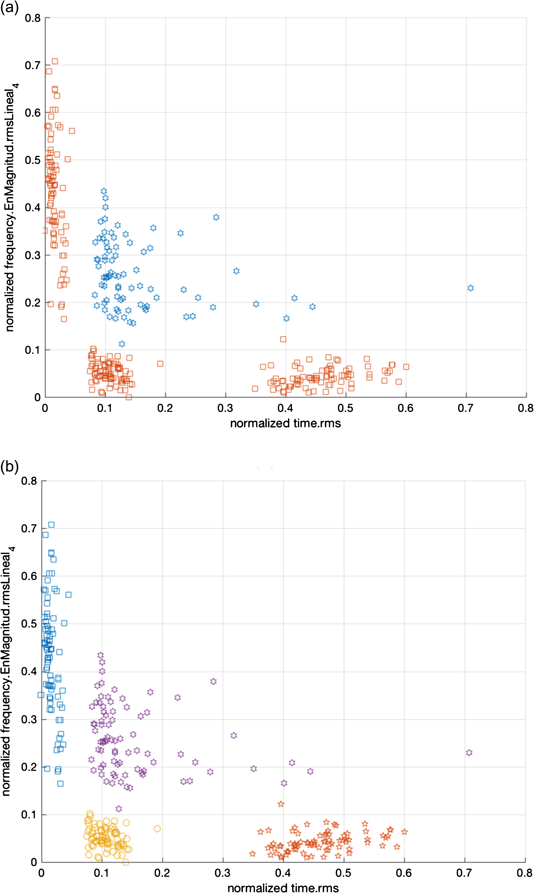
Ground truth partitions for (a) 2 clusters, i.e., fault/no fault case, and (b) for 4 clusters corresponding to the 4 health conditions of the CWRU setup. Data points represented with the same graphical symbol belong to the same cluster.

Fig.2

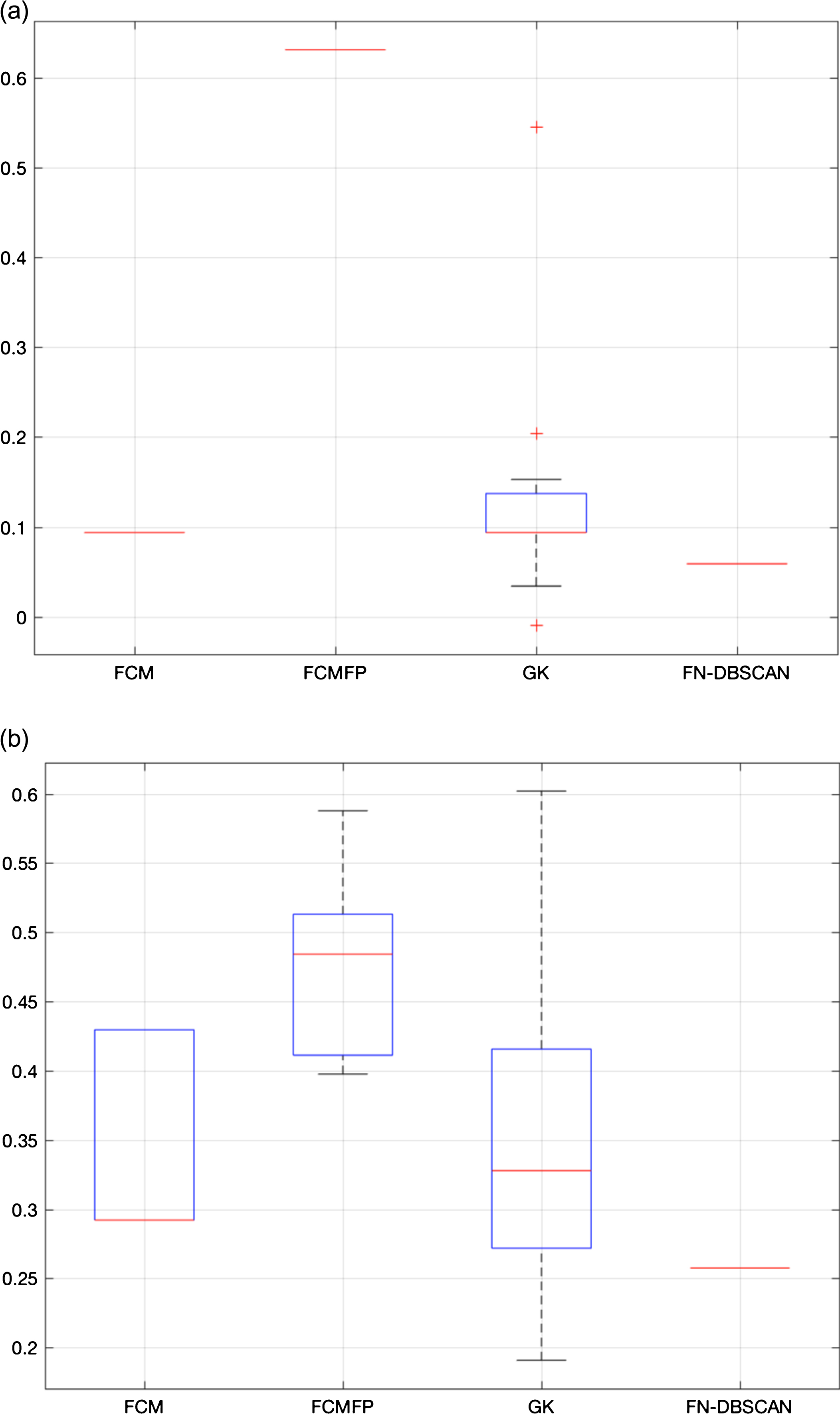
Boxplots showing the dispersion of the Rand Index values obtained by the algorithms over 30 independent runs for (a) 2 and (b) 4 clusters – CWRU setup.

Table 2

The hyper-parameters used in the algorithm comparison for the CWRU setup. $\bar{X}$ stands for the data baricenter

Ground	FCM		GK			FCMFP			FN-DBSCAN
truth	m	C	m	C	ρ _i	m	P	ζ	ε	ν
2 clusters	2.0	2	2.0	2	1.0	2.0	$[\bar{X} 10]$	0.5	0.98	20
4 clusters	2.0	4	2.0	4	1.0	2.0	$[\bar{X} 10]$	0.08	0.9976	1

The four algorithms were compared against external validation and the observed dispersion of Rand Index values are displayed in Fig. 4. A pf = 1.7e - 17 and pf = 1.2e - 18 were obtained for (a) 2 and (b) 4 clusters, respectively, meaning that there is a statistical significant difference among the results of the algorithms in both cases. Further analysis reveals that for (a) the best performance was due to FN-DBSCAN and the worst to FCM. For (b) the best was GK while the worst was FN-DBSCAN. The hyper-parameters used by the algorithms in the comparison are presented in Table 3. FCM and GK were the easiest algorithms to configured while the other two were the hardest. As no systematic method was available for tuning the algorithms, no claim can be made on the optimality of used hyper-parameters is made. The FN-DBSCAN algorithm is the only one the ability to detect outliers in the dataset and is immune to initial conditions.

Fig.3

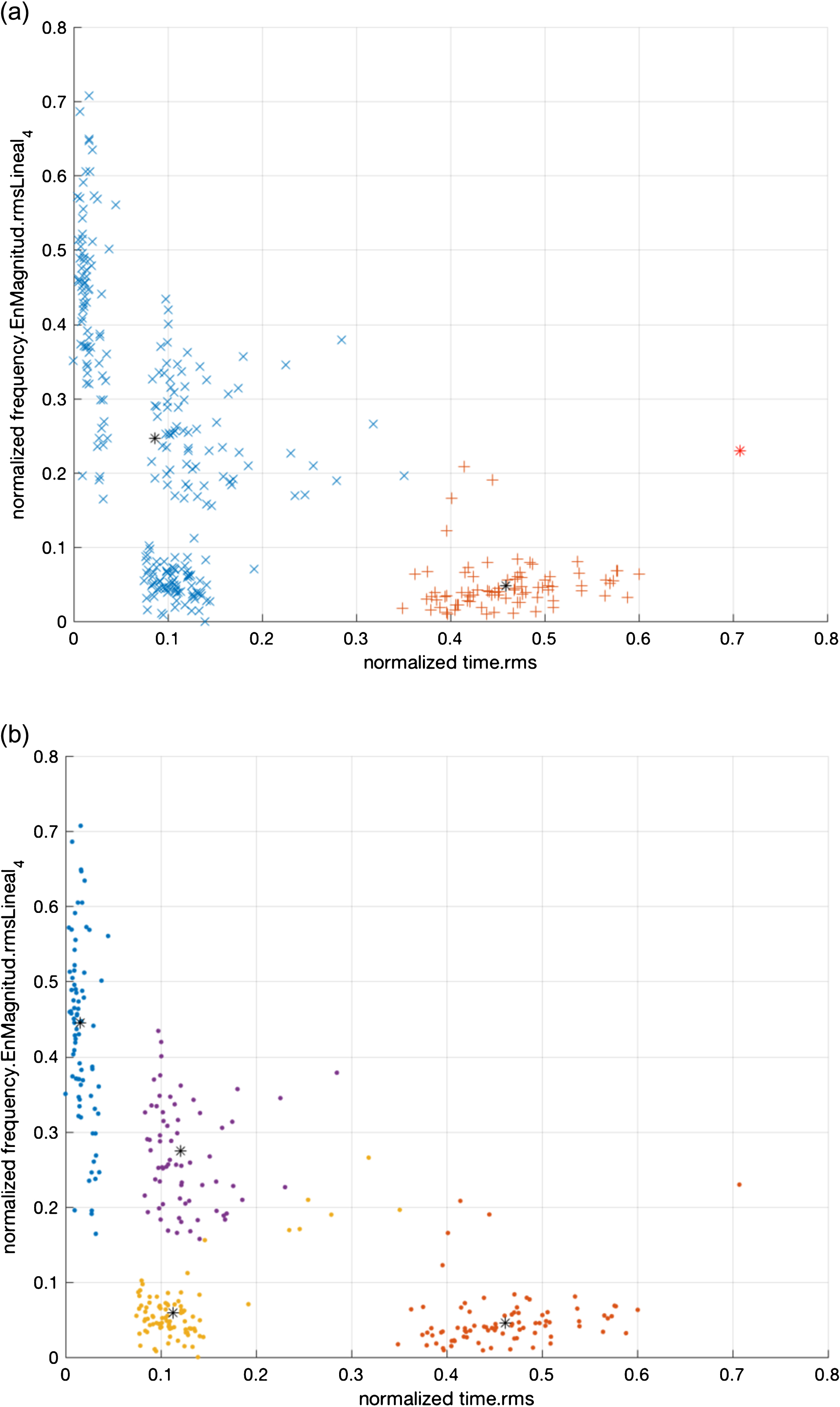
Best clustering results as evaluated by the Rand Index for the CWRU setup: (a) FN-DBSCAN 2 clusters and (b) GK with 4 clusters. Cluster centers are identified by the symbol * and outliers by *. Otherwise, each cluster is identified by data points represented by the same graphical symbol.

Figure 3 shows the best clustering results obtained for (a) 2 clusters (FN-DBSCAN) and (b) 4 clusters (GK).

4.2 Results for the GIDTEC setup

Fig.4

Boxplots showing the dispersion of the Adjusted Rand Index values obtained by the algorithms over 30 independent runs for (a) 2 and (b) 7 clusters – GIDTEC stepup.

Table 3

The hyper-parameters used in the algorithm comparison for the GIDTEC setup. $\bar{X}$ stands for the data baricenter

Ground	FCM		GK			FCMFP			FN-DBSCAN
truth	m	C	m	C	ρ _i	m	P	ζ	ε	ν
2 clusters	2.0	2	2.0	2	1.0	2.0	$[\bar{X} 10]$	0.95	0.9683	10
7 clusters	2.0	7	2.0	7	1.0	2.0	$[\bar{X} 10]$	0.13	0.992	10

Fig.5

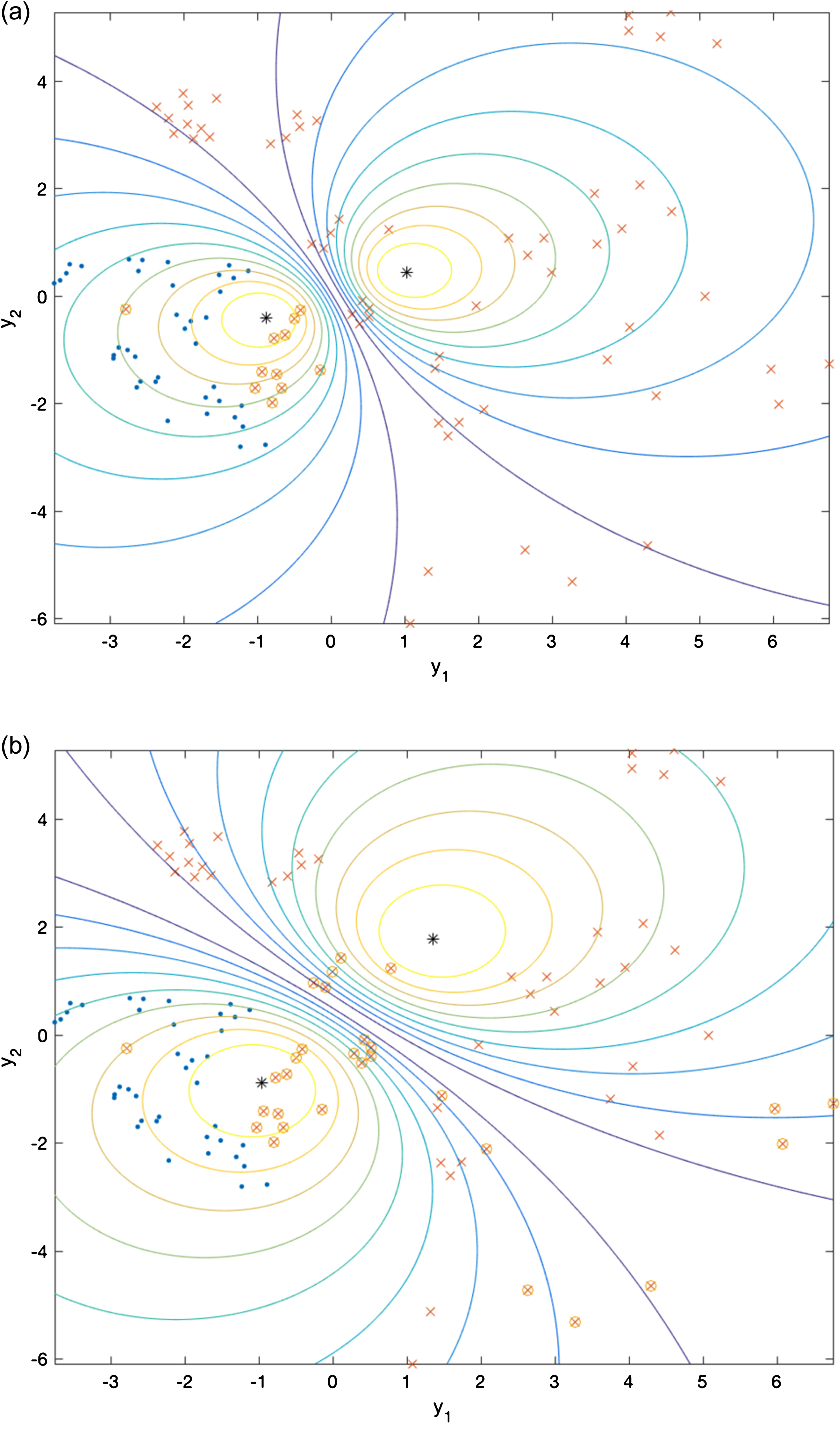
Sammon projections of the 12 dimensions feature space into the plane showing the best clustering results for the GIDTEC setup with 2 clusters obtained by (a) FCMFP and (b) GK. Cluster centers are identified by the symbol *. Otherwise, each cluster is identified by the same graphical symbol.

Fig.6

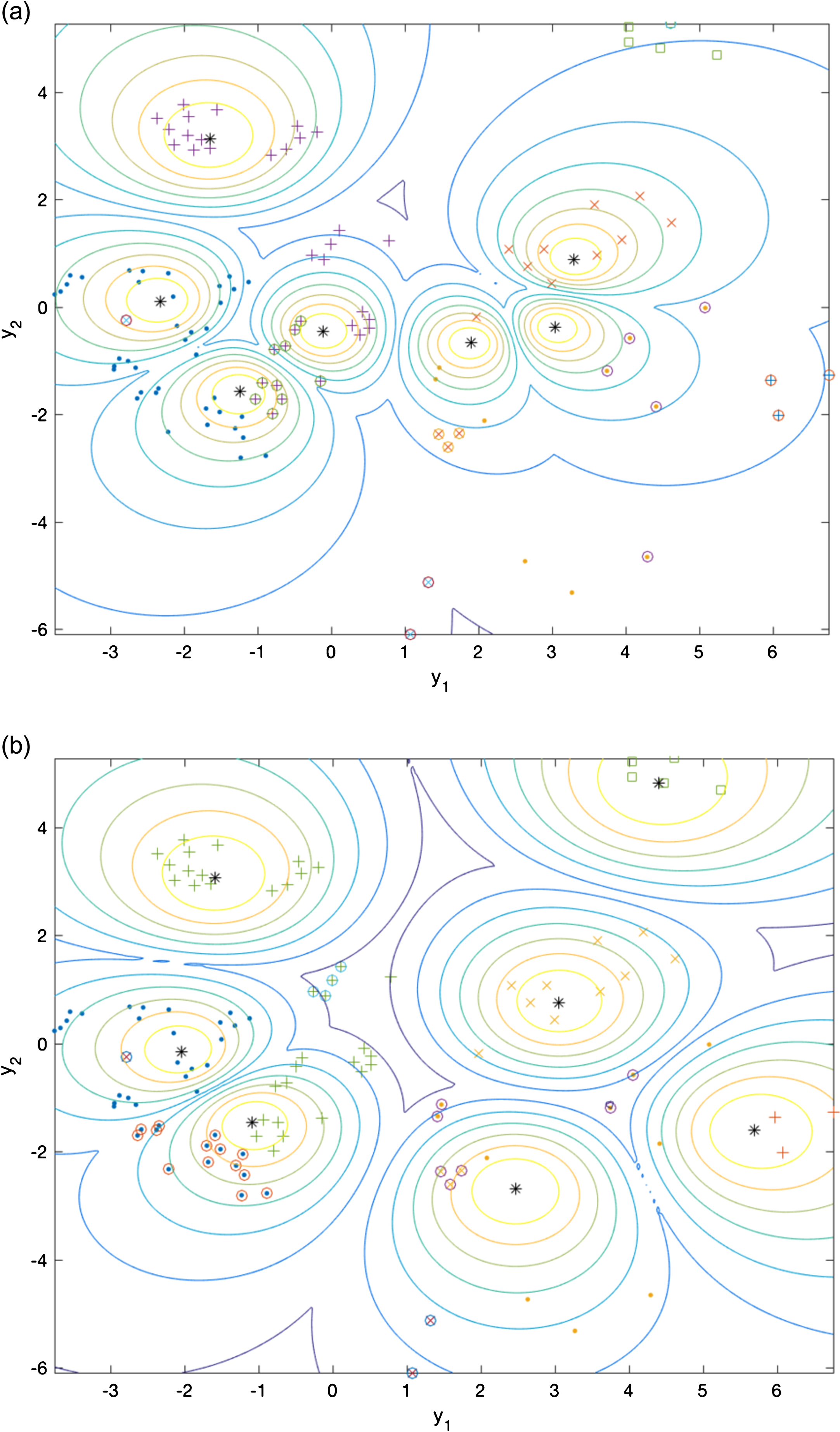
Sammon projections of the 12 dimensions feature space into the plane showing typical clustering results obtained by FCMFP for the GIDTEC setup with 7 clusters. Cluster centers are identified by the symbol *. Otherwise, each cluster is identified by the same graphical symbol. The focal point is located in (a) the baricenter of the data and (b) over the point where features are maximal. Different levels of detail are observed depending on the position of the focal point.

When the proposed methodology is applied to the data set acquired with this setup only 12 relevant features out of 1634 are selected as the most relevant. Other methods such as those based on genetic algorithms selected a number of features one order of magnitude higher typically. From the selected features one can see that Accelerometer 1 is responsible for capturing 9 out of the 12 selected features. Wavelets, i.e., time-frequency domain features correspond to 5 of the total number of selected features; In addition, five time domain and three frequency domain features have been selected. See [6, 11] for details. The four algorithms were compared against external validation and the observed dispersion of Adjusted Rand Index values are displayed in Fig. 4. A pf = 1.35e - 16 and pf = 1.8e - 12 were obtained for (a) 2 and (b) 7 clusters, respectively, meaning that there is a statistical significant difference among the results of the algorithms in both cases. Further analysis reveals that for both (a) and (b) the best performance was due to FCMFP.

The hyper-parameters used are presented in Table 3. As before, FCM and GK were the easiest to configured algorithms while the FCMFP and FN-DBSCAN were the hardest. Again, no claim on the optimality of used hyper-parameters can be made.

Figure 5 shows Sammon projections of the 12-dimensional feature space into the plane. In this figure, the centers of each cluster are denoted by the symbol *. Around each cluster center there are ten solid line curves with different colors ranging from yellow to dark blue, each one of them representing a contour of equal membership value; the farthest the curve from the center the lower the membership value (the darker the blue the lower the membership). Each one of the other colored symbols represents to the truth classification of a sample. Samples in the same class are represented by the same color and symbol. In this figure one can see the best partition produced by (a) FCMFP and (b) by GK for 2 clusters.

Figure 6 shows typical clustering results obtained by FCMFP for 7 clusters. In (a) the focal point is located in over the data baricenter and in (b) it is located over the point where all features attain their maximum values. As it can be seen by changing the focal point it is possible to obtain different levels of detail in different regions of the feature space.

It seems than the shrinkage technique based on which FCMFP is designed plays an important role in multi-dimensional features spaces as is the case of this setup. Curiously enough, this type of performance improvement was not the primary goal beyond FCMFP but appears as a convenient side-effect [15].

It is likely that the relative poor performance of FN-DBSCAN is due to the difficulty of finding a convenient parametrization of the algorithm for this particular data set. It is well-known that the algorithm is highly sensitive to the employed membership function (13) as well as to the thresholds ε and ν.

5 Conclusions

Bearing fault diagnosis is recognized as both an economically relevant and technical challenging problem. Fuzzy clustering has been extensively exploited in the bearing fault diagnosis literature, especially by resorting to the well-known FCM algorithm. However, up to now no study on the comparison of the rich variety of clustering algorithms has been conducted in bearing diagnosis. In order to bridge this gap, this paper has presented a first-time comparison of four representative algorithms: FCM, GK, FCMFP, and FN-DBSCAN.

To ensure operating conditions as realistic as possible, the studied considered only real-world bearing vibration data coming from both the CWRU benchmark data set and from a more challenging GIDTEC setup specially developed by our research group where fault interferences, different loading conditions, and high levels of noise can be studied.

The comparison takes into account the quality of the generated partitions measured by the external quality Rand and Adjusted Rand indexes. Statistical tests of hypothesis revealed that for the CWRU setup where only two features were used to characterize the bearing healthy state, FN-DBSCAN and GK exhibit the best performance for 2 clusters (fault/no fault case) and for 4 clusters, respectively.

In the GIDTEC setup 12 features were used to identify seven different bearings states. In this case, FCMFP outperformed all the other for both the fault/no fault case and for 7 clusters. The design principle beyond this algorithm is to allows the user to select a suitable level of granularity in a given region of the feature space. However results shown that FCMFP produces partitions exhibiting better external validity index values than the corresponding unbiased algorithm (FCM) for any number of clusters. The improvement is viewed as a convenient side effect of the shrinkage technique employed in the design of the algorithm. From this perspective, one can claim that works currently employing FCM in bearing fault diagnosis would benefit from the use of FCMFP. This also suggests that extension of GK and FN-DBSCAN algorithms with the same design principle and shrinkage technique could also improve the performance of that algorithms in this type of problem.

Footnotes

Acknowledgments

The work was sponsored in part by the Prometeo Project of the Secretariat for Higher Education, Science, Technology and Innovation (SENESCYT) of the Republic of Ecuador, the National Key Research & Development Program of China (2016YFE0132200), and by Fundação para a Ciência e Tecnologia (FCT), Portugal. The experimental work was developed at the GIDTEC research group lab of UPS, Cuenca, Ecuador.

Appendix

References

Valente de Oliveira

, and Pedrycz

, Advances in Fuzzy Clustering and Its Applications. New York, NY, USA: John Wiley & Sons, Inc, 2007.

, Valente de Oliveira

, Cerrada

, Pacheco

, Cabrera

, Vinicio Sanchez

and Zurita

, A systematicreview of fuzzy formalisms for bearing fault diagnosis,, Submitted, 2017.

Jiang

, Liu

, Li

and Chen

, Degradation assessment and fault diagnosis for roller bearing based on armodel and fuzzy cluster analysis, Shock and Vibration18(1-2) (2011), 127–137.

Lotfan

, Salehpour

, Adiban

and Mashroutechi

, Bearingfault detection using fuzzy C-means and hybrid C-means-subtractivealgorithms, 2015 IEEE International Conference on FuzzySystems (FUZZ-IEEE)2015, 1–7.

Han

, Li

, Zhan

and Li

X.L.

, Rolling bearing fault diagnosis method based on EEMD permutation entropy andfuzzy clustering, in pp, 2015 Fifth International Conference on Instrumentation and Measurement, Computer, Communication and Control (IMCCC)2015, 470–474.

, Valente de Oliveira

, Cerrada

, Pacheco

, Cabrera

, V. Sanchez and Zurita

, Observer-biasedbearing condition monitoring: From fault detection to multi-fault classification, Engineering Applicationsof Artificial Intelligence. 287–301. 50 (2016), http://www.sciencedirect.com/science/article/pii/S0952197616000427.

, Lin

T.R.

and Tan

J.W.

, A bearing fault diagnosis technique based on singular values of EEMD spatial condition matrix and gath-geva clustering, http://www.sciencedirect.com/science/article/pii/S682X, Applied Acoustics121180433–45.

Zhang

, Ma

and He

, Fault diagnosis model based on fuzzy support vector machine combined with weighted fuzzy clustering, Transactions of Tianjin University19(3) (2013), 174–181.

Vijay

, Pai

, Sriram

and Rao

, Bearing diagnostics - a radial basis function neural network approach, Proceedings of the International Conference on Condition Monitoring and Diagnostic Engineering Management(COMADEM)2011, 843–854.

10.

Vijay

, Pai

, Sriram

and Rao

, Radial basis function neural network based comon of dimensionality reduction techniquesfor effective bearing diagnostics, Proceedings of the Institution of Mechanical Engineers, Part J: ParisJournalof Engineering Tribology227(6) (2013), 640–653.

11.

, Ledo

, Delgado

, Cerrada

, Pacheco

, Cabrera

, Sanchez

and Valente

, de Oliveira, A bayesianapproach to parameter estimation in probabilistic fuzzy systems and its application to bearing fault diagnosis, [Online]. Knowledge-Based Systems2017, Knowledge-Based Systems2017, 10.1016/j.knosys.2017.05.007

12.

Pan

Y.S.N.

and Yi

, Rolling bearing faults detection based on improved sparse component analysis, in pp, 2016 IEEE International Conference on Information and Automation (ICIA)2016, 772–775.

13.

Gustafson

and Kessel

, Fuzzy clustering with a fuzzy covariance matrix, IEEE Conference on Decisionand Control Including the 17th Symposium on Adaptive Processes, 1978, 761–766.

14.

Fazendeiro

and Valente de Oliveira

, A fuzzy clustering algorithm with a variable focal point, 2008 IEEE International Conference on Fuzzy Systems (IEEE World Congress on Computational Intelligence), 2008, 1049–1056.

15.

Fazendeiro

and Valente de Oliveira

, Observer-biased fuzzy clustering, Fuzzy Systems, IEEE Transactions on23(1) (2015), 85–97.

16.

Nasibov

E.N.

and Ulutagay

, Robustness of density-based clustering methods with various neighborhood relations, Fuzzy Sets and Systems160(24) (2009), 3601–3615.

17.

Ulutagay

and Nasibov

, Fuzzy and crisp clustering methods basedon the neighborhood concept: A comprehensive review, J IntellFuzzy Syst23(6) (2012), 271–281.

18.

Loparo

, Bearings vibration data set. The Case Western Reserve University Bearing Data Center, http://www.eecs.cwru.edu/laboratory/bearing/download.htm, 2011].

19.

MacQueen

, Some methods for classification and analysis ofmultivariate observations, L.M. Le Cam and J. Neyman, Eds. Berkeley,CA, USA, Proceedings of the 5th Berkeley Symposium on Mathematical Statistics and Probability1University of California Press, Berkeley, CA, USA, 1967, 281–297.

20.

Fazendeiro

, Valente de Oliveira

, Fuzzy clustering as a datadriven development environment for information granules, Handbook of Granular ComputingW. Pedrycz, A. Skowron and V. Kreinovich, John Wiley & Sons, Ltd, 2008, 153–169.

21.

Farajzadeh-Zanjani

, Razavi-Far

, Saif

, Zarei

and Palade

, Diagnosis of bearing defects in induction motors by fuzzy neighborhood density-based clustering, in pp, 2015 IEEE 14th International Conference on Machine Learning and Applications (ICMLA)2015, 935–940.

22.

, Sanchez

, Zurita

, Lozada

M.C.

and Cabrera

, Rolling element bearing defect detection using thegeneralized synchrosqueezing transform guided by time-frequency ridge enhancement, ISA Transactions602487, 274–284. http://www.sciencedirect.com/science/article/pii/

23.

, Cabrera de Oliveira

, Valente

, Sanchez

R.-V.

, Cerrada

and Zurita

, Extracting repetitivetransients for rotating machinery diagnosis using multiscale clustered grey infogram, Mechanical Systems andSignal Processing7677 (2016), 157–173. [Online]. Available: http://www.sciencedirect.com/science/article/pii/S0888327016001151

24.

, Valente de Oliveira

, Sánchez

, Cerrada

, G. Zurita and Cabrera

, Fuzzy determination ofinformative frequency band for bearing fault detection, Journal of Intelligent and Fuzzy Systems30(6) (2016), 3513–3525. http://dx.doi.org/10.3233/IFS-162097

25.

Cerrada-Lozada

, Sánchez

R.-V.

, Li

, Pacheco

, Cabrera

and Valente

, de Oliveira, A review ondata-driven fault severity assessment in bearings, Mechanical Systems and Signal Processing, submitted.

26.

Pacheco

, Valente de Oliveira

, Snchez

R.-V.

, Cerrada

, Cabrera

, Li

, G. Zurita and Arts

, Astatistical comon of neuroclassifiers and feature selection methods for gearbox fault diagnosis underrealistic conditions, http://www.sciencedirect.com/science/article/pii/, Neurocomputing1942016, 192–206.

27.

Sheskin

, Handbook of Parametric and Nonparametric Statistical Procedures, Fifth Edition, ser. A Chapman & Hall book. Taylor & Francis2011, https://books.google.com.ec/books?id=YDd2cgAACAAJ.

28.

Hubert

and Arabie

, Comparing partitions, Journal of Classification2(1) (1985), 193–218. http://dx.doi.org/10.1007/BF01908075

A comparison of fuzzy clustering algorithms for bearing fault diagnosis

Abstract

Keywords

1 Introduction

2 Background: The clustering methods

2.1 FCM

3.1 Experimental apparatus

3.1.1 The CWRU setup

3.1.2 The GIDTEC setup

Table 1 Health states of the essayed bearings for the GIDTEC setup Id Bearing 1 Bearing 2 P1 healthy healthy P2 inner race fault healthy P3 outer race fault healthy P4 ball fault healthy P5 inner race fault outer race fault P6 inner race fault ball fault P7 outer race fault ball fault

3.3 Features selection

4 Results and discussion

4.1 Results for the CWRU setup

Footnotes

Acknowledgments

Appendix

References

Table 1
Health states of the essayed bearings for the GIDTEC setup

Id Bearing 1 Bearing 2

P1 healthy healthy

P2 inner race fault healthy

P3 outer race fault healthy

P4 ball fault healthy

P5 inner race fault outer race fault

P6 inner race fault ball fault

P7 outer race fault ball fault