A dual-objective vendor-managed inventory model for a single-vendor multi-retailersupply chain with fuzzy random demand

Abstract

This paper develops a dual-objective vendor-managed inventory model with a single supplier and multiple retailers in a supply chain in which the retailer’s demand is assumed as a fuzzy random variable and the supplier incurs a constant deterioration rate. The model is optimized to simultaneously minimize the total cost and maximize the service level under capital budget and storage constraints, in which ordering cost, holding cost, deterioration cost and transportation cost are considered in the total cost of the vendor. To solve the proposed model in an imprecise environment, the expected value and pessimistic value are used to change the fuzzy random model into a determined model. Three fuzzy random simulations are presented to obtain the optimal replenishment quantities of the expectation model and the pessimistic model. A numerical study with a single vendor and three retailers in the supply chain is provided to demonstrate the efficiency of the models and algorithms, which gives the optimal results for the expectation model and pessimistic model. Furthermore, recommendations for the replenishment policy for different types of decision makers in the pessimistic model are provided based on the analysis of inventory costs with different parameter values.

Keywords

Vendor-managed inventory supply chain fuzzy random demand expected value pessimistic value

1 Introduction

In the 21st century, competition is no longer among individual enterprises, it is among supply chains. As a vital part of supply chain management, effective inventory management and stock control have attracted increasing attention. Vendor-managed inventory (VMI) is an efficient method which makes the inventories of the supplier and retailer integrally managed through information sharing and cooperation. The retailers share sale data and inventory information using an information system such as Electronic Data Interchange and Internet-based XML protocols. The supplier undertakes the responsibility of replenishment, inventory management and distribution of retailers based on the information. VMI system is a complicated business entity and has a high degree of uncertainty. There are three different sources of uncertainty, including supplying, process and demand uncertainty. This article considers the demand uncertainty in modeling which aims to reduce the impact of fluctuations on suppliers and whole supply chain and find an optimal stock strategy in a VMI system with a single vendor and multi-retailer.

Most scholars studied stock control problem considering the retailer’s demand as a random variable [1 –3]. Kiesmuller [4] developed a two-echelon inventory system for a single supplier and a single retailer. The demand of the retailer was assumed as a random variable, and the aim was to obtain the minimum total cost of supply chain with an economic order quantity. Lan [5] had a deep research in stock control problem of deteriorating products in the VMI model with multiple retailers and considered the stochastic demand. A bi-level programming model was established with minimal cost and delivery time.

With the development of uncertainty theory, the fuzzy variable was used to study the inventory model for the VMI problem. Tong [6] proposed a VMI model consisted of a single factory and a single customer with a triangular fuzzy demand and obtained the maximum profit of the supply chain. Sadeghi [7] constructed an economic production quantity VMI model in multi-retailer single-supplier supply chain management under storage capacity, replenishment quantity and average stock capacity limitations. Sadeghi [8] developed a bi-objective model where the demand was a fuzzy variable and the supplier managed the retailer’s inventory in a middle stockroom. The optimal result was to determine the replenishment frequency, minimizing stock cost and storage area of the retailer. In a study by Nia [9], the retailers’ demand, supplier’s storage capacity and ordering quantity were considered fuzzy, and the proposed model was intended to obtain the minimal total cost of the supply chain.

The uncertain random theory was introduced in inventory management and stock control considering the fuzzy and random features of demand. In a study by Li [10], there were optimistic, pessimistic and risk-neutral decision indexes when making replenishment decision. And retalier’s demand was recognized as a fuzzy random variable in a supply chain coordinated by a buyback contract. Zhang [11] conducted a model based on the study [10], and the cost of backorder was added to the profit model. A realistic case was introduced to demonstrate the efficiency of supply chain coordination and the effect of mixed imprecise and uncertain demand. Hu [12] studied a two-stage supply chain system including a single customer and a single vendor for deteriorating items where the demand was considered a triangular fuzzy variable. Expectation theory and signed distance were applied to change the fuzzy random model into a deterministic model, which maximized the total profit with the optimal initial order quantity. Nagar [13] established a multi-objective two-echelon stochastic programming supply chain model with uncertain producing rate, imprecise vendor productivity and fuzzy random demand. The maximum return, maximum customer service level, and minimum decision risk were determined at the end of the paper. Chakraborty [14] considered the following factors to be fuzzy random and bifuzzy: the price of product, holding cost, procurement cost, transportation cost, storage area and capital budget. A model with stock deterioration for a multi-item supply chain was optimized to determine the credit periods and total time of the supply chain cycle with limited storage space and budget.

Table 1 summarizes the related literatures for the supply chain modeled in an imprecise environment. As is shown in Table 1, many domestic and international scholars only considered random demand or fuzzy demand when it came to the VMI problem in an imprecise environment; Only a few literatures established the multi-objective model and considered deterioration in modeling. In this article, a dual-objective VMI model is developed where retailers demand is assumed as a fuzzy random demand and the deterioration is considered in the calculation process of stock status and costs related to inventory. The proposed model is optimized to obtain the appropriate replenishment quantity which intends to get the minimum total cost and the maximum service ability.

Table 1
Summary of related literature for the supply chain model in an imprecise environment

Author IE IP O V/R C D ST T

Mateen [1] Only Random Demand S S/M No No Yes No

Lee [2] Only Random Demand S S/S No No Yes No

Nagarajan [3] Only Random Demand S S/S No No Yes No

Kiesmuller [4] Only Random Demand S S/S No No Yes Yes

Lan [5] Only Random Demand M S/M No Yes No Yes

Tong [6] Only Fuzzy Demand S S/S No No No No

Sadeghi [7] Only Fuzzy Demand S S/M Yes No No Yes

Sadeghi [8] Only Fuzzy Demand M S/M Yes No No No

Nia [9] Only Fuzzy Demand S S/S Yes No Yes No

Storage area

Oder quantity

Li [10] Fuzzy Random Demand S S/S No No No No

Zhang [11] Fuzzy Random Demand S S/S No No Yes No

Hu [12] Fuzzy Random Demand S S/S No Yes Yes No

Nagar [13] Fuzzy Random Demand M M/M Yes No Yes Yes

Production rate

Supplier capacity

Chakraborty [14] Fuzzy Random&Bifuzzy Cost S S/S Yes Yes Yes Yes

Storage area

Budget

Proposed model Fuzzy Random Demand M S/M Yes Yes Yes Yes

Author	IE	IP	O	V/R	C	D	ST	T
Mateen [1]	Only Random	Demand	S	S/M	No	No	Yes	No
Lee [2]	Only Random	Demand	S	S/S	No	No	Yes	No
Nagarajan [3]	Only Random	Demand	S	S/S	No	No	Yes	No
Kiesmuller [4]	Only Random	Demand	S	S/S	No	No	Yes	Yes
Lan [5]	Only Random	Demand	M	S/M	No	Yes	No	Yes
Tong [6]	Only Fuzzy	Demand	S	S/S	No	No	No	No
Sadeghi [7]	Only Fuzzy	Demand	S	S/M	Yes	No	No	Yes
Sadeghi [8]	Only Fuzzy	Demand	M	S/M	Yes	No	No	No
Nia [9]	Only Fuzzy	Demand	S	S/S	Yes	No	Yes	No
		Storage area
		Oder quantity
Li [10]	Fuzzy Random	Demand	S	S/S	No	No	No	No
Zhang [11]	Fuzzy Random	Demand	S	S/S	No	No	Yes	No
Hu [12]	Fuzzy Random	Demand	S	S/S	No	Yes	Yes	No
Nagar [13]	Fuzzy Random	Demand	M	M/M	Yes	No	Yes	Yes
		Production rate
		Supplier capacity
Chakraborty [14]	Fuzzy Random&Bifuzzy	Cost	S	S/S	Yes	Yes	Yes	Yes
		Storage area
		Budget
Proposed model	Fuzzy Random	Demand	M	S/M	Yes	Yes	Yes	Yes

IE: Imprecise Environment; IP: Imprecise Parameter; O: Objective; V/R: Vendor/Retailer; C: Constraint; D: Deterioration; ST: Shortage; T: Transportation; S: Single; M: Multi.

The rest of the article is structured as following five parts. Section 2 represents the definitions and theorems in the developed model. The problem description and principal assumptions are provided in Section 3. Section 4 illustrates the dual-objective VMI model in detail, and three fuzzy random simulation algorithms are proposed in Section 5. Section 6 includes a numerical study for the expectation model and pessimistic model, and the optimal result is presented. Finally, the conclusion and future research are discussed at the end of this paper.

2 Theory

In the paper, a dual-objective VMI model with fuzzy random demand is proposed and uncertainty theory developed by Liu is applied to the process of model constructing and solving. The definitions and theorems needed in this paper are as followings.

Definition 1. An uncertain random variable is function ξ. From a chance space (Γ, L, M) × (Ω, A, Pr) to the set of real numbers, such that ξ ∈ B is an event in L × A for any Borel set B of real numbers.

Definition 2. [15] Let ξ_i be uncertain random variables in the probability space (Ω_i, A_i, Pr _i), i = 1, 2, ⋯ n, and let f : Rⁿ → R be a measurable function. Then, ξ = f (ξ₁, ξ₂, ⋯, ξ_n) is an uncertain random variable in the product probability spaces (Ω₁ × Ω₂ × ⋯ × Ω_n, A₁ × A₂ × ⋯ × A_n, Pr ₁ × Pr ₁ × ⋯ × Pr _n), and $\begin{matrix} ξ (ω_{1}, ω_{2}, \dots, ω_{n}) \\ = f (ξ_{1} (ω_{1}), ξ_{2} (ω_{2}), \dots, ξ_{n} (ω_{n})) \end{matrix}$ for all (ω₁, ω₂, ⋯, ω_n) ∈ Ω₁ × Ω₂ × ⋯ × Ω_n.

Definition 3. [15] Let ξ be an uncertain random variable. Then, its expected value is defined by $\begin{matrix} E [ξ] & = & \int_{0}^{\infty} Pr {ω \in Ω | E [ξ (ω)] \geq r} d r \\ - \int_{- \infty}^{0} Pr {ω \in Ω | E [ξ (ω)] \leq r} d r \end{matrix}$ if at least one of the two integrals is finite.

Theorem 1. [15] Letξandηbe uncertain random variables with finite expected values. ξ (ω) andη (ω) are independent; for allω ∈ Ω, a and b are real numbers; then $E [a ξ + b η] = aE [ξ] + bE [η]$

Definition 4. [16] Let ξ be an uncertain random variable, and γ, δ ∈ (0, 1]; then $ξ_{inf} = inf {r | Ch {ξ \leq r} (γ) \geq δ}$ is defined as (γ, δ) pessimistic value of uncertain random variable ξ.

Definition 5. [17] Let ξ be an uncertain random variable in the probability space (Ω, A, Pr) and B be a Borel set of real numbers; then $Ch {ξ \in B} (α) = sup_{Pr {A} \geq α} inf_{ω \in A} Cr {ξ (ω) \in B}$ is defined as the chance value of event ξ ∈ B.

Theorem 2. [17] Letξbe a n uncertain random variable in the probability space (Ω, A, Pr) and B be a Borel set of real numbers, for allα^* ∈ (0, 1], setβ^* = Ch {ξ ∈ B} (α^*); then $Pr {ω \in Ω | Cr {ξ (ω) \in B} \geq β^{*}} \geq α^{*}$

3 Problem definition and assumptions

The vendor-managed inventory system with a single supplier and multi-retailer is proposed in Fig. 1. The supply chain includes a single supplier and multiple retailers who face multiple sale seasons. The vendor provides a single product to all customers according to their orders and undertakes the responsibility of replenishment, stock management and distributions. The model only considers the process of procurement, storage and distribution; the manufacturing procedure is neglected.

Fig.1

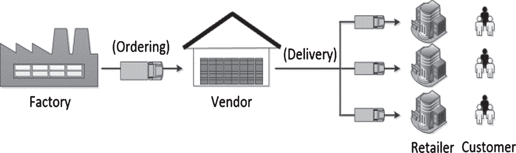
An illustration of a supply chain.

The amounts of vendor’s inventory and retailer’s inventory are presented in Fig. 2, where the retailer’s demand is considered fuzzy random and the supplier’s stock deteriorates at a fixed rate. The supplier’s demand is equal to the accumulation of all retailer demand in the supply chain in a replenishment interval, and the supplier satisfies m replenishment cycles of retailers with the initial ordering quantity.

Fig.2

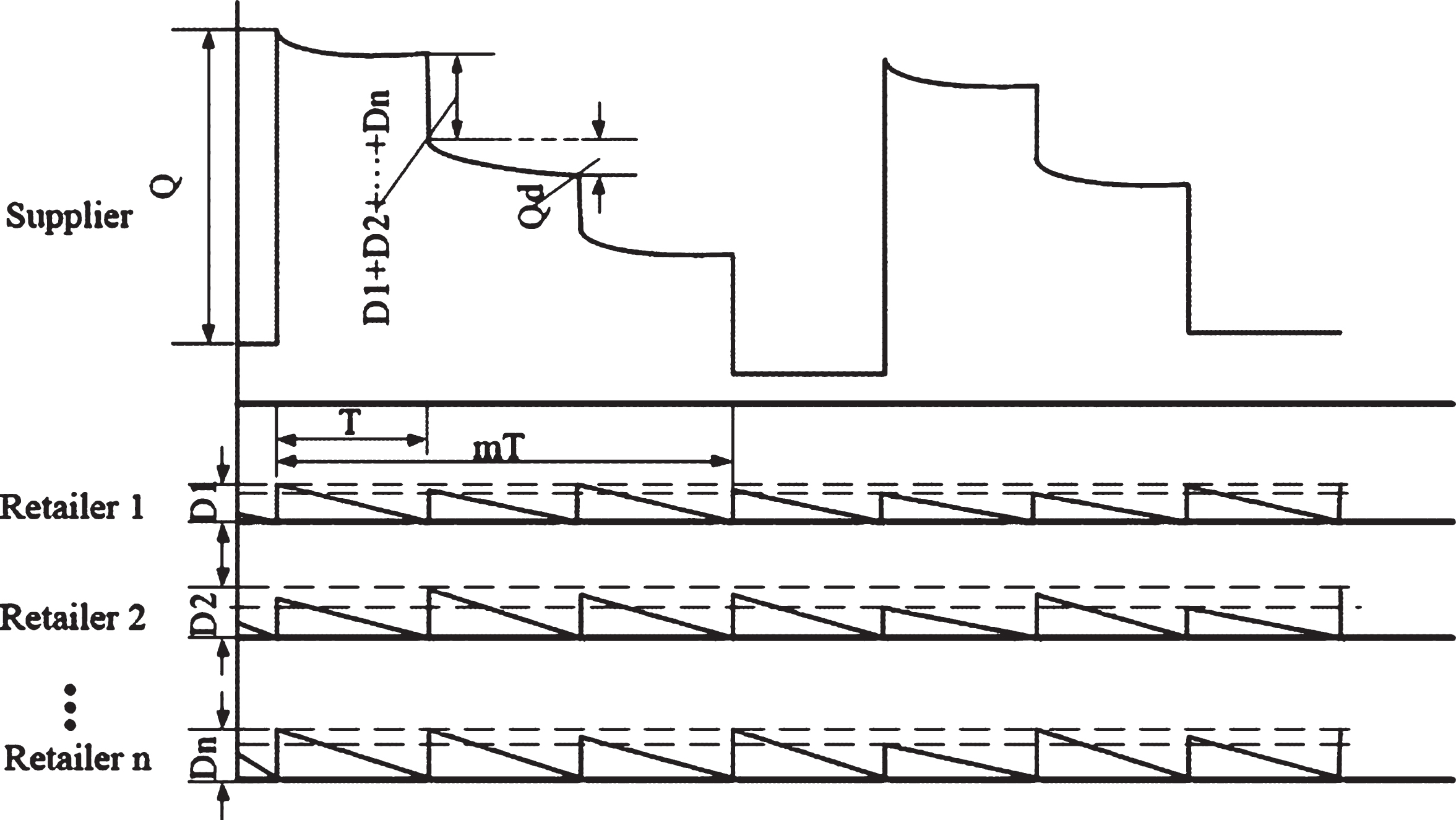
Inventory levels with single vendor and multiple retailers.

The principal assumptions which the proposed VMI model with the fuzzy random demand considered is based on are as follows:

There is a supply chain, which consists of a single supplier and multi-retailer, and the supplier only provides a single item for all retailers.

The retailer’s demands are independent, and the supplier replenishes retailers at the same time.

All products are owned by the supplier until the delivery is completed, and all retailers have no inventory.

The storage time of the retailer is notably short, and holding cost can be neglected.

The vendor is responsible for the deterioration of products in the process of procurement, storage and distribution.

The ordering quantity of the supplier should satisfy multiple replenishments of retailers and the reorder point is zero.

Shortages are only permitted in the last replenishment cycle, which corresponds to the supplement period of the vendor.

The price of the product, fixed cost of ordering and shipment, variable cost of shipment, holding cost per unit, existing inventory, deteriorated rate, capital budget and storage space are constant.

4 VMI model formulation

4.1 Notations and demand descriptions

Notations involved in this paper are shown as followings.

C_O replenishment cost of the vendor

$\tilde{\bar{C_{H}}}$ stock holding cost of the vendor

$\tilde{\bar{C_{D}}}$ deterioration cost of the vendor

$\tilde{\bar{C_{T}}}$ delivery cost of the vendor

${\tilde{\bar{C}}}_{Total}$ total cost of the vendor

R_cost maximum amount of financial resources

R_space maximum amount of spatial resources

$\tilde{\bar{D_{i}}}$ actual demand for retailer i

$\tilde{\bar{S_{j}}}$ supplied quantity of the vendor in period j

Q ordering quantity per time of the vendor

I_e existing inventory of the vendor

$\tilde{\bar{I_{j}}}$ amount of inventory of vendor before period j

$\tilde{\bar{Q_{d}^{j}}}$ deterioration of products of the vendor in period j

$\tilde{\bar{Q_{d}}}$ deteriorated quantity of products in all replenishment cycles

$\tilde{\bar{Q_{s}}}$ shortage of products of the vendor

h holding cost per unit during one period

θ deterioration rate of the item

c price of commodity per unit

c_o fixed cost per order of vendor

c_f fixed cost per shipment

c_v transportation cost per unit

n number of retailers in supply chain

m replenishment cycles for retailers

The retailer’s demand fluctuates in practical situations and it’s always not completely consistent with supplier’s prediction. Because of the lead time of production, there are many cases when the supplier cannot satisfy the actual demands of the retailers. The demands might be less, equal or more than expected, and the probability of these cases can be obtained from historical data. However, there are little or no available data to support decision and two reasons are accountable for this phenomenon. For one thing, the environment always changes in the supply chain. for another, the existing data cannot accurately estimate the probability distribution of the retailer actual need in the supply chain [18]. Hence, the demand described with a single random variable or a single fuzzy variable is not suited. To solve the uncertainties of the retailer’s demand and quickly respond to the diverse demand, a fuzzy random variable is applied to the proposed model and it is much more accurate to reflect environment changes in this complicated situation.

The fuzzy random demand of retailer i is denoted by ${\tilde{\bar{D}}}_{i}$ as Equation (1), the fuzzy demand of retailer i in case ω_n is denoted by $\tilde{d_{i}^{n}}$ , and the probability is p_n ${\tilde{\bar{D}}}_{i} = {\begin{matrix} \tilde{d_{i}^{1}} & ω = ω_{1} & p_{1} \\ \tilde{d_{i}^{2}} & ω = ω_{2} & p_{2} \\ ⋮ & ⋮ & ⋮ \\ \tilde{d_{i}^{n}} & ω = ω_{n} & p_{n} \end{matrix}$ (1)

4.2 Objectives and constraints

The supplier undertakes the costs of management and deterioration in the process of procurement, storage and distribution in the proposed model. The vendor may lose sale opportunities and even customers when a shortage is incurred. Therefore, a dual-objective VMI model is composed according to the assumptions and derivations in Section 3. The objectives are as follows: (1) minimization of the total cost of the supplier; (2) maximization of the service ability for the retailers. The model aims to obtain the optimal replenishment quantity under the budget and space constraints.

The inventory level with deterioration can be described by Equation (2) according to [5] when the demand is zero. $\frac{dI (t)}{dt} = - θ I (t)$ (2)

The amount of inventory of the vendor at time t in the replenishment cycle j of retailers is shown in Equation (3). $I (t) = I ((j - 1) T) e^{- θ (t - (j - 1)) T} t \in [(j - 1) T, jT]$ (3)

The stock status and deteriorated quantities at the end of the replenishment periods of retailers are expressed in the following segmented Equations (4 and 5), respectively. Then, j < m, $\tilde{\bar{S_{j}}} = \sum_{i = 1}^{n} \tilde{\bar{D_{i}}}$ ; j = m, $\tilde{\bar{S_{j}}} = min {\sum_{i = 1}^{n} \tilde{\bar{D_{i}}}, {\tilde{\bar{I}}}_{j - 1}}$ .

$I_{j} = {\begin{matrix} (Q + I_{e}) e^{- θ} & j = 1 \\ (Q + I_{e}) e^{- 2 θ} - \tilde{\bar{S_{1}}} e^{- θ} - \tilde{\bar{S_{2}}} & j = 2 \\ ⋮ \\ (Q + I_{e}) e^{- m θ} - \sum_{k = 1}^{m} \tilde{\bar{S_{k}}} e^{- (m - k) θ} & j = m \end{matrix}$ (4) ∥ $Q_{d}^{j} = {\begin{matrix} (Q + I_{e}) (1 - e^{- θ}) & j = 1 \\ [(Q + I_{e}) e^{- θ} - \tilde{\bar{S_{1}}}] (1 - e^{- θ}) & j = 2 \\ ⋮ \\ [(Q + I_{e}) e^{- (m - 1) θ} - \sum_{k = 1}^{m - 1} \tilde{\bar{S_{k}}} e^{- (m - 1 - k) θ}] (1 - e^{- θ}) & j = m \end{matrix}$ (5) ∥The total cost of the vendor is shown in Equation (6), which includes the ordering cost, holding cost, delivery cost and deterioration cost. ${\tilde{\bar{C}}}_{Total} = C_{O} + \tilde{\bar{C_{H}}} + \tilde{\bar{C_{T}}} + \tilde{\bar{C_{D}}}$ (6) ∥The replenishment cost per cycle for the vendor is expressed in Equation (7), which includes fixed replenishment costs and transportation cost from the factory to the warehouse. $C_{O} = c_{o} + c_{v} \times Q$ (7) ∥The holding cost is given in Equation (8).∥ $\tilde{\bar{C_{H}}} = h \times (\tilde{\bar{I_{1}}} + \tilde{\bar{I_{2}}} + \dots + \tilde{\bar{I_{m}}}) = \frac{h}{(1 - e^{- θ})} [(Q + I_{e}) (1 - e^{- m θ}) - \sum_{j = 1}^{m} \tilde{\bar{S_{j}}} (1 - e^{- (m - j + 1) θ})]$ (8) ∥The distribution cost is given in Equation (9), which consists of the fixed cost of the vehicle and the variable aspect; t is the number of retailers whose demand can be satisfied.∥ $\begin{matrix} \tilde{\bar{C_{T}}} & = & \sum_{j = 1}^{m} (n^{'} c_{f} + c_{v} \tilde{\bar{S_{j}}}) \\ = & [(m - 1) \times n + t] c_{f} + c_{v} \sum_{j = 1}^{m} \tilde{\bar{S_{j}}} \end{matrix}$ (9) ∥The deterioration cost is expressed with the value of deteriorated products in Equation (10) based on the deteriorated quantity proposed in Equation (5). $\tilde{\bar{C_{D}}} = c \times \sum_{j = 1}^{m} \tilde{\bar{Q_{d}^{j}}} = c \times [(Q + I_{e}) (1 - e^{- m θ}) - \sum_{j = 1}^{m - 1} \tilde{\bar{S_{j}}} (1 - e^{- (m - j) θ})]$ (10) ∥Finally, the total cost is given in Equation (11). $\begin{matrix} {\tilde{\bar{C}}}_{Total} \\ = C_{O} + {\tilde{\bar{C}}}_{H} + {\tilde{\bar{C}}}_{T} + {\tilde{\bar{C}}}_{D} \\ = c_{o} + [c_{v} + \frac{h (1 - e^{- m θ})}{(1 - e^{- θ})} + c (1 - e^{- m θ})] Q \\ + [\frac{h (1 - e^{- m θ})}{(1 - e^{- θ})} + c (1 - e^{- m θ})] I_{e} \\ - \frac{h}{(1 - e^{- θ})} \sum_{j = 1}^{m} \tilde{\bar{S_{j}}} (1 - e^{- (m - j + 1) θ}) + c_{v} \sum_{j = 1}^{m} \tilde{\bar{S_{j}}} \\ - c \sum_{j = 1}^{m - 1} \tilde{\bar{S_{j}}} (1 - e^{- (m - j) θ}) + [(m - 1) \times n + t] c_{f} \end{matrix}$ ∥The service level is commonly measured by the availability of the product. The supplier may permanently lose the sale opportunities and customer in the case of shortage. The quantity of supplier’s shortage is selected to evaluate the service level as shown in Equation (12). $\begin{matrix} Q_{s} \end{matrix} & & = max {0, \sum_{j = 1}^{m} \sum_{i = 1}^{n} \tilde{\bar{D_{i}}} - Q - I_{e} + \sum_{j = 1}^{m} \tilde{\bar{Q_{d}^{j}}}} & & = max {0, \sum_{j = 1}^{m} \sum_{i = 1}^{n} (\begin{matrix} \tilde{\bar{D_{i}}} - (Q + I_{e}) e^{- m θ} - \\ \sum_{j = 1}^{m - 1} \tilde{\bar{S_{j}}} (1 - e^{- (m - j) θ}) \end{matrix})} & &$ ∥With these derivations, the VMI model with fuzzy random demand under the budget and space constraints is shown in Equation (13).∥ $\begin{matrix} min {\tilde{\bar{C}}}_{Total} \\ min \tilde{\bar{Q_{s}}} \\ s . t \\ c \times Q + {\tilde{\bar{C}}}_{Total} \leq R_{cost} \\ \sum_{j = 1}^{m - 1} (\tilde{\bar{S_{j}}} + \tilde{\bar{Q_{d}^{j}}}) \leq I_{e} + Q \leq R_{space} \end{matrix}$ (11) ∥

4.3 Expectation model (Model_1)

The expectation model of uncertain random variable proposed by Liu [19] is applied to obtain the optimal solutions of the proposed VMI model. Since the objectives are conflicting, there are no optimal solution which simultaneously minimizes the total cost and shortage. With the increment of replenishment quantity, the shortage will decrease. However, the total cost of the vendor will increase. To obtain the optimal result, the second objective is converted into a constraint of the first objective; then, λQ expresses the allowable shortage of the supplier, and λ ∈ [0, 1]. The minimum expected total cost for the VMI problem under the budget and space constraints is expressed in Equation (14).∥ $\begin{matrix} min E [{\tilde{\bar{C}}}_{Total}] \\ s . t \\ c \times Q + E [{\tilde{\bar{C}}}_{Total}] \leq R_{cost} \\ E [\tilde{\bar{Q_{s}}}] \leq λ Q \\ \sum_{j = 1}^{m - 1} (E [\tilde{\bar{S_{j}}}] + E [\tilde{\bar{Q_{d}^{j}}}]) \leq I_{e} + Q \leq R_{space} \end{matrix}$ (12) ∥∥ $E [\tilde{\bar{Q_{s}}}]$ and $E [{\tilde{\bar{C}}}_{Total}]$ are denoted in Equations (15 and 16), respectively; then, j < m, $E [\tilde{\bar{S_{j}}}] = \sum_{i = 1}^{n} E [\tilde{\bar{D_{i}}}]$ ; otherwise, $E [\tilde{\bar{S_{j}}}] = min {\sum_{i = 1}^{n} E [\tilde{\bar{D_{i}}}], E [{\tilde{\bar{I}}}_{j - 1}]}$ .∥ $\begin{matrix} E [\tilde{\bar{Q_{s}}}] \\ = max {0, \sum_{j = 1}^{m} \sum_{i = 1}^{n} E [\tilde{\bar{D_{i}}}] - Q - I_{e} + \sum_{j = 1}^{m} E [\tilde{\bar{Q_{d}^{j}}}]} \\ = max {0, \sum_{j = 1}^{m} \sum_{i = 1}^{n} (\begin{matrix} E [\tilde{\bar{D_{i}}}] - e^{- m θ} (Q + I_{e}) - \\ \sum_{j = 1}^{m - 1} E [\tilde{\bar{S_{j}}}] (1 - e^{- (m - j) θ}) \end{matrix})} \end{matrix}$ (13) ∥ $\begin{matrix} E [{\tilde{\bar{C}}}_{Total}] \\ = E [C_{O}] + E [{\tilde{\bar{C}}}_{H}] + E [{\tilde{\bar{C}}}_{T}] + E [{\tilde{\bar{C}}}_{D}] \\ = c_{o} + [c_{v} + \frac{h (1 - e^{- m θ})}{(1 - e^{- θ})} + c (1 - e^{- m θ})] Q \\ + [\frac{h (1 - e^{- m θ})}{(1 - e^{- θ})} + c (1 - e^{- m θ})] I_{e} + c_{v} \sum_{j = 1}^{m} E [\tilde{\bar{S_{j}}}] \\ - \frac{h}{(1 - e^{- θ})} \sum_{j = 1}^{m} E [\tilde{\bar{S_{j}}}] (1 - e^{- (m - j + 1) θ}) \\ - c \sum_{j = 1}^{m - 1} E [\tilde{\bar{S_{j}}}] (1 - e^{- (m - j) θ}) + [(m - 1) \times n + t] c_{f} \end{matrix}$ (14) ∥

4.4 Pessimisticmodel (Model_2)

The chance constraint model with the minimum pessimism value of the fuzzy random variable, which was proposed by Liu, is used to get the optimal solutions of the VMI problem [16]. The original model is converted to achieve the minimum pessimistic value of the total cost, where the second objective of shortage becomes a chance constraint at the allowable shortage quantity; λQ is the allowable shortage quantity of the supplier, and λ ∈ [0, 1]. The pessimistic model under the chance constraint is expressed in Equation (17). This model aims to determine the minimum total cost under budget and space constraints, where the chance of shortage is less than the permitted value which is greater than σ.∥∥ $\begin{matrix} min C_{inf} \\ s . t \\ Ch {{\tilde{\bar{C}}}_{Total} ⩽ C_{inf}} (γ) ⩾ δ \\ Ch {\tilde{\bar{Q_{S}}} ⩽ λ Q} (α) ⩾ σ \\ c \times Q + C_{inf} ⩽ R_{cost} \\ \sum_{j = 1}^{m - 1} (\tilde{\bar{S_{j}}} + \tilde{\bar{Q_{d}^{j}}}) ⩽ I_{e} + Q ⩽ R_{space} \end{matrix}$ (15) indent According to the definition of the pessimistic value and α - chance in literatures [16, 17].∥Equation (17) is equivalent to Equation (18). $\begin{matrix} min C_{inf} \\ s . t \\ Pr {ω_{1} \in Ω | Cr {{\tilde{\bar{C}}}_{Total} ⩽ C_{inf}} ⩾ δ} ⩾ γ \\ Pr {ω_{2} \in Ω | Cr {\tilde{\bar{Q_{S}}} - λ Q ⩽ 0} ⩾ β} ⩾ α ⩾ σ \\ c \times Q + C_{inf} ⩽ R_{cost} \\ \sum_{j = 1}^{m - 1} (\tilde{\bar{S_{j}}} + \tilde{\bar{Q_{d}^{j}}}) ⩽ I_{e} + Q ⩽ R_{space} \end{matrix}$ (16)

5 Fuzzy random simulations

To solve the proposed models, three algorithms are developed:

Fuzzy random simulation for the expected value

Fuzzy random simulation for the pessimistic value

Fuzzy random simulation for the α - chance value

f (ω_{i}) = \sum_{k = 1}^{n} D_{k} (ω_{i})

is a fuzzy random variable; if D_k (ω_i) is a fuzzy random variable, then f (ω_i) = (l₁, l₂, l₃) and its membership function is expressed in Equation (19).

μ (f (ω_{i})) = {\begin{matrix} \frac{f - l_{1}}{l_{2} - l_{1}} & if l_{1} \leq f \leq l_{2} \\ \frac{f - l_{3}}{l_{2} - l_{3}} & if l_{2} \leq f \leq l_{3} \\ 0 & otherwise \end{matrix}

(17)

5.1 Algorithm 1 Fuzzy random simulation for the expected value

Step 1. Set E = 0;

Step 2. Randomly generate sample ω_i according to the probability distribution Pr;

Step 3. Calculate E [f (ω_i)];

Set e = 0;

Randomly generate fuzzy variables f_j (ω_i) with membership degrees μ_j, j = 1, 2 ⋯ N;

Calculate the minimum and maximum values $\begin{matrix} a & = & min {f_{j} (ω_{i}) | 1 \leq j \leq N}, \\ b & = & max {f_{j} (ω_{i}) | 1 \leq j \leq N}; \end{matrix}$

Uniformly generate r from the range [a, b];

If r ≥ 0 set $\begin{matrix} e = e + Cr {f_{j} (ω_{i}) \geq r}, \\ Cr {f_{j} (ω_{i}) \geq r} \\ = \frac{1}{2} (max_{f_{j} (ω_{i}) \geq r} μ_{j} + 1 - min_{f_{j} (ω_{i}) < r} μ_{j}) \end{matrix}$

If r < 0 $\begin{matrix} e = e - Cr {f_{j} (ω_{i}) \leq r}, \\ Cr {f_{j} (ω_{i}) \leq r} \\ = \frac{1}{2} (max_{f_{j} (ω_{i}) \leq r} μ_{j} + 1 - min_{f_{j} (ω_{i}) > r} μ_{j}) \end{matrix}$

Repeat (4) and (5) N times; the expected value is $\begin{matrix} E [f (ω_{i})] \\ = max {a, 0} + min {b, 0} + e \times (b - a) / N \end{matrix}$

Step 4. Set E = E + E [f (ω_i)]; and

Step 5. Repeat Steps 2–4 N times; the expected value of the fuzzy random variable is E [f (ω)] = E/N.

5.2 Algorithm 2 Fuzzy random simulation for the pessimistic value

Step 1. Randomly generate sample $ω_{i} = {ω_{i 1}, ω_{i 1}, \dots, ω_{im}}$ according to the probability distribution Pr;

Step 2. Calculate $\bar{F_{i}} = inf {F_{i} | Cr {F (f (ω_{i})) \leq \bar{F_{i}}} \geq δ}$ apply the fuzzy simulation;

Initialize ɛ, which is a small positive number;

Randomly generate the fuzzy vectors $f (ω_{i 1}), f (ω_{i 2}), \dots, f (ω_{im})$ with membership degrees μ_i1, μ_i2, ⋯, μ_im;

Let the fuzzy variable be $F (ω_{i}) = F (f (ω_{i 1}), f (ω_{i 2}), \dots, f (ω_{im}))$ with membership degree μ_i = min {μ_i1, μ_i2, ⋯, μ_im};

Repeat (2) and (3) N times;

Calculate the minimum and maximum values: $\begin{matrix} a & = & min {F_{j} (ω_{i}) | 1 \leq j \leq N}, \\ b & = & max {F_{j} (ω_{i}) | 1 \leq j \leq N} . \end{matrix}$

Set r = (a + b)/2;

Calculate the credibility $L (r) = \frac{1}{2} (max_{F_{j} (ω_{i}) \leq r} μ_{j} + 1 - min_{F_{j} (ω_{i}) > r} μ_{j})$

If L (r) ≥ δ, set b = r; otherwise, set a = r;

If b - a ≥ ɛ, go to step (6); and

Return r as the δ pessimistic value of variable F (ω_i).

Step 3. Repeat Steps 1 and 2 N times, let N′ be the integer portion of γN; and

Step 4. Return sequence ${\bar{F_{1}}, \bar{F_{2}} \dots \bar{F_{N}}}$ ; the N′ largest element is considered the (γ, δ) pessimistic value of fuzzy randomvariable F.

5.3 Algorithm 3 Fuzzy random simulation for the α - chance value

Step 1. Randomly generate samples ω₁, ω₁, ⋯, ω_N according to the probability distribution Pr;

Step 2. Calculate $β_{i} = Cr {g (\tilde{Q_{S}} (ω_{i})) \leq 0}, i = 1, 2 \dots N;$ apply the fuzzy simulation; then $g (\tilde{Q_{S}} (ω_{i})) = \tilde{Q_{S}} (ω_{i}) - λ Q$

Set j = 1;

Randomly generate the fuzzy vectors $g (\tilde{Q_{S}} (ω_{i}))$ with membership degrees μ_j;

j = j + 1; if j ≤ N, go to step (2); otherwise, go to step (4); and

Calculate and return β_i; then $\begin{matrix} β_{i} & = & \frac{1}{2} (max {μ_{j} | g (\tilde{Q_{S}} (ω_{i})) \leq 0} \\ + min {1 - μ_{j} | g (\tilde{Q_{S}} (ω_{i})) > 0}) \end{matrix}$

Step 3. Let be intact part of αN; and

Step 4. Return the N′ largest element in ${β_{1}, β_{2}, \dots β_{N}} .$

6 Numerical Study

To illustrate the application of the proposed model and algorithms and investigate its performances, a supply chain with a single supplier and three retailers is assumed. The cost of different procedures and resource constraints are shown in Table 2 and demands of retailers are shown in Table 3. Model_1 is solved by Algorithm 1, and Model_2 is solved by Algorithm 2 and Algorithm 3. All the solutions are obtained by thesoftwareMATLAB2012a on a personal computer.

Table 2
Input data in a fuzzy random environment

Prameter Value Prameter Value

R _cost 2.500,000 c _o 5,000

R _space 260,000 c _f 500

I _e 1,000 c _v 1

c 100 θ 0.01

h 1 m 5

Prameter	Value	Prameter	Value
R _cost	2.500,000	c _o	5,000
R _space	260,000	c _f	500
I _e	1,000	c _v	1
c	100	θ	0.01
h	1	m	5

Note: The unit of all kinds of cost is yuan (RMB).

Table 3

Demands of retailers in a fuzzy random environment

Retailer_1		Retailer_2		Retailer_3
1,000	1,200	2,000	2,400	600	900
1,100	1,300	2,200	2,500	800	1,000
1,200	1,400	2,400	2,600	900	1,100
0.8	0.2	0.6	0.4	0.7	0.3

6.1 Optimal result of Model_1

The optimal result of Model_1 is shown in Fig. 3. The expected total cost is an increasing function of replenishment quantity, whereas the expected shortage is a decreasing function of the initial order quantity. The expected quantity of shortage is zero if the replenishment quantity is greater than 21,263 units. The ordering quantity of the supplier is optimal if the shortage quantity is equal to the allowance. The allowable quantity of shortage is decided by decision maker. In the case of λ = 0.1, the optimal replenishment quantity is 19,241 units at the intersection point of the left vertical line and the x-axis, and the expected shortage is 1,924 units. Additionally, the minimum expected total cost is 144,751 yuan. Similarly, the optimum initial quantity occurs at the intersection point of the right vertical line and the x-axis in the case of λ = 0.05, and the optimum order quantity, minimum expected total cost and expected shortage of products are 20,202 units, 154,780 yuan and 1,009 units, respectively. The optimal result is shown in Table 4.

Fig.3

Optimal result of model_1.

Table 4

Optimal result of Model_1

λ	Order Quantity	Total Cost	Shortage
0.5	20,202	154,780	1,009
0.1	19,241	144,751	1,924

Note: The unit of total cost is yuan (RMB).

6.2 Optimal result of Model_2

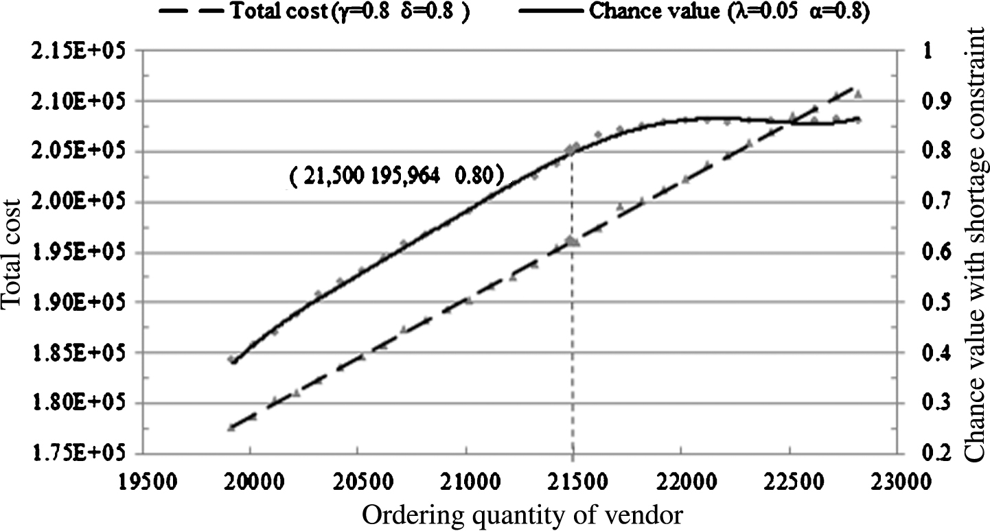
The optimal result of Model_2 is shown in Fig. 4 for γ = 0.8, δ = 0.8, α = 0.8 and λ = 0.1. With the increase in initial ordering quantity, the total cost increases nearly linearly, whereas the chance value first increases and gradually remains stable. The intersection point of the vertical line and total cost curve represents the minimum cost of the supplier when σ is equal to 0.8. The optimal replenishment quantity is 20,470 units, the minimum total cost of the supplier is 184,211 yuan. Similarly, the supplier’s total cost curve and the chance value curve with the shortage constraint when λ = 0.05 is shown in Fig. 5, where the optimum ordering quantity and total cost of σ = 0.8 are 21,500 units and 195,964 yuan, respectively. The optimal result of Model_2 for various values of parameters λ and σ is shown in Table 5.

Fig.4

Optimal result of model_2 (λ = 0.1).

Fig.5

Optimal result of model_2 (λ = 0.05).

Table 5

Optimal result of Model_2

γ= 0.8 δ= 0.8 α= 0.8	ChanceValue	Order Quantity	Total Cost
λ= 0.1	σ= 0.85	20,792	187,954
	σ= 0.80	20,470	184,211
	σ= 0.75	20,254	181,556
	σ= 0.70	20,095	180,029
λ= 0.05	σ= 0.85	21,770	199,830
	σ= 0.80	21,500	195,965
	σ= 0.75	21,320	193,819
	σ= 0.70	21,087	191,157

Note: The unit of total cost is yuan (RMB).

The result of Model_2 when γ = 0.8, δ = 0.8 and α = 0.8 is more reliable than the other model with smaller parameter values. There is a slight possibility that the shortage is greater than the permitted value with the optimal replenishment quantity, but the total cost is relatively higher. As a result, it is suitable for risk-averse entrepreneurs. The values of parameters γ and δ can decrease to reduce the total cost for a risk-preference decision maker. As is shown in Figs. 6 and 7, the total cost decreases when the values of parameters γ and δ are reduced. The functions of the total cost with various values of δ are shown in Fig. 6, where γ is equal to 0.8. Similarly, the functions of the total cost with various values of γ are shown in Fig. 7, where δ is equal to 0.8. With the decrease in α, the optimal replenishment quantity and total cost decrease because of the increase in α - chance. The optimal results of the α - chance value with the shortage constraint for various α values are shown in Figs. 8 and 9. Although the optimal ordering quantity and total cost decrease with smaller values of parameters γ, δ and α for Model_2, the credibility of the model is undermined, and the shortage risk increases.

Fig.6

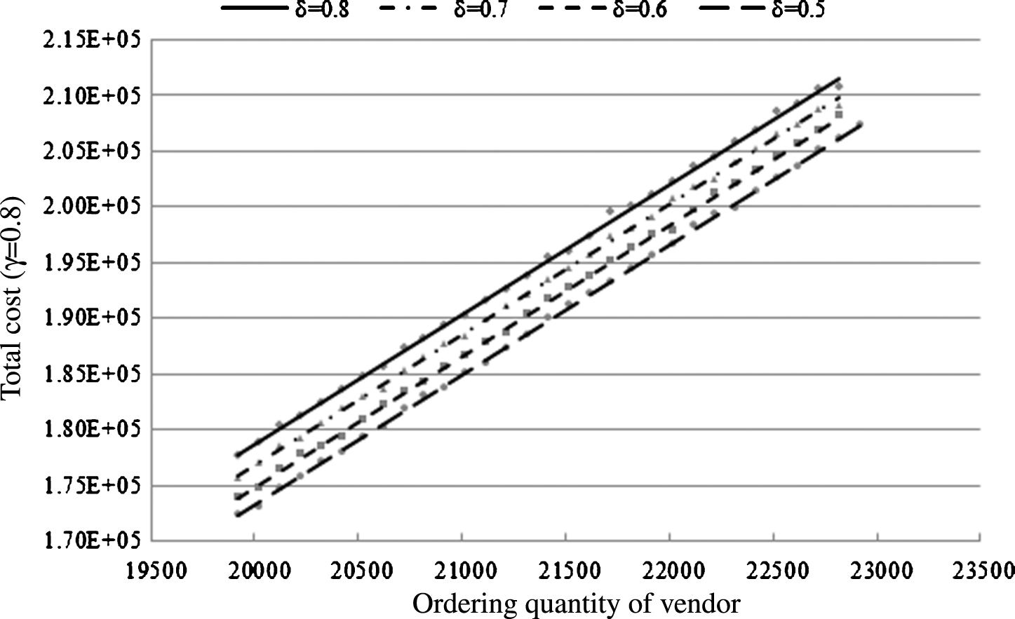
Pessimistic value of the total cost (γ = 0.8).

Fig.7

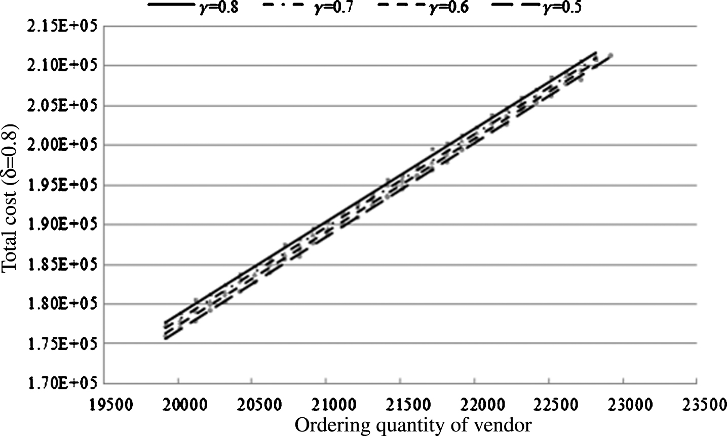
Pessimistic value of the total cost (δ = 0.8).

Fig.8

Chance value with shortage constraint (λ = 0.1).

Fig.9

Chance value with shortage constraint (λ = 0.05).

7 Conclusion

In this paper, a vendor-managed inventory model for a single supplier and multiple retailers with fuzzy random demand is proposed. The proposed model aims to obtain the minimal total cost and maximal degree of service under budget and space constraints. The expectation model and pessimistic model are used to obtain the optimal solutions. The fuzzy random model for the VMI problem is transformed into a deterministic model with expectation in which the replenishment quantity of the supplier is determined by the historical sale data of retailers and realistic environment. Therefore, the simulation results are more suitable for the practical situation. The pessimism model provides the optimal replenishment quantity and minimal pessimistic value of the total cost in terms of the retailer’s demand under budget, space and shortage constraints in case of credibility δ and probability γ. Some features of this model are as follows: (1) It is a dual-objective VMI model with total cost minimization and service ability maximization for multiple retailers under multiple constraints. (2) The retailer’s demand, which is described with the fuzzy random variable, exactly reflects real life. (3) The stock deterioration and delivery process are considered in this model, meanwhile the deterioration cost and distribution cost are included in the total cost. The present model can be extended to a multi-supplier and multi-retailer model with multiple items in future studies, and the deterioration rate can be considered a variable value.

References

Mateen

, Chatterjee

A.K.

and Mitra

, VMI for single-vendor multi-retailer supply chains under stochasticdemand[J], Computers & Industrial Engineering79 (2015), 95–102.

Lee

J.Y.

and Ren

, Vendor-managed inventory in a global environment with exchange rate uncertainty[J], International Journal of Production Economics130 (2011), 169–174.

Nagarajan

and Rajagopalan

, Contracting under vendor managed inventory systems using holding cost subsidies[J], Production & Operations Management17 (2008), 200–210.

Kiesmüller

G.P.

and Broekmeulen

R.A.C.M.

, The benefit of VMI strategies in a stochastic multi-product serial two echelon system[J], Computers & Operations Research37 (2010), 406–416.

Lan

H.J.

, Li

R.X.

, Liu

Z.G.

, Study on the inventory control of deteriorating items under VMI model based on bi-level programming[J], Expert Systems with Applications38 (2011), 9287–9295.

Tong

and Zhao

D.Z.

, A Supply Chain Model of Vendor Managed Inventory with Fuzzy Demand[C], International Conference on System Science, Engineering Design and Manufacturing Informatization IEEE Computer Society2 (2010), 15–18.

Sadeghi

, Sadeghi

and Niaki

S.T.A.

, Optimizing a hybrid vendor-managed inventory and transportation problem with fuzzy demand: An improved particle swarm optimization algorithm[J], Information Sciences272 (2014), 126–144.

Sadeghi

and Niaki

S.T.A.

, Two parameter tuned multi-objective evolutionary algorithms for a bi-objective vendor managed inventory model with trapezoidal fuzzy demand[J], Applied Soft Computing Journal30 (2015), 567–576.

Nia

A.R.

, Far

M.H.

and Niaki

S.T.A

, A fuzzy vendor managed inventory of multi-item economic order quantity modelunder shortage: An ant colony optimization algorithm[J], International Journal of Production Economics155 (2014), 259–271.

10.

and Zhao

, Supply Chain Real Time Coordination Method Based on Buyback Contract with Fuzzy Random Demand[C], IEEE International Conference on Fuzzy Systems IEEE (2006) pp.1543–1549.

11.

Zhang

, Lu

, Zhang

, Supply chain coordination based on a buyback contract under fuzzy random variable demand[J], Fuzzy Sets & Systems255 (2014), 1–16.

12.

J.S.

, Zheng

, Xu

R.Q.

, Supply chain coordination for fuzzy newsboy problem with imperfect quality[J], International Journal of Information & Management Sciences51 (2010), 771–784.

13.

Nagar

, Dutta

and Jain

, An integrated supply chain model for new products with imprecise production and supply under scenario dependent fuzzy random demand[J], International Journal of Systems Science45 (2012), 873–887.

14.

Chakraborty

, Jana

D.K.

and Roy

T.K.

, Multi-item integrated supply chain model for deteriorating items with stock dependent demand under fuzzy random and bifuzzy environments [J], Computers & Industrial Engineering88 (2015), 166–180.

15.

Liu

Y.K.

and Liu

B.D.

, Fuzzy random variables: A scalar expected value operator[J], Fuzzy Optimization & Decision Making2 (2003), 143–160.

16.

Liu

B.D.

, Fuzzy random chance-constrained programming[J], IEEE Transactions on Fuzzy Systems9 (2001), 713–720.

17.

Gao

J.W.

and Liu

B.D.

, New primitive chance measures of fuzzy random event[J], International Journal of Fuzzy Systems3 (2001), 527–531.

18.

Xie

, Petrovic

and Burnham

, A heuristic procedure for the two-level control of serial supply chains under fuzzy customer demand[J], International Journal of Production Economics102 (2006), 37–50.

19.

Liu

Y.K.

and Liu

B.D.

, A class of fuzzy random optimization: Expected value models[J], Information Sciences An International Journal155 (2003), 89–102.

A dual-objective vendor-managed inventory model for a single-vendor multi-retailersupply chain with fuzzy random demand

Abstract

Keywords

1 Introduction

3 Problem definition and assumptions

4.1 Notations and demand descriptions

5.2 Algorithm 2 Fuzzy random simulation for the pessimistic value

5.3 Algorithm 3 Fuzzy random simulation for the α - chance value

6 Numerical Study

Table 2 Input data in a fuzzy random environment Prameter Value Prameter Value R cost 2.500,000 c o 5,000 R space 260,000 c f 500 I e 1,000 c v 1 c 100 θ 0.01 h 1 m 5

References

Table 2
Input data in a fuzzy random environment

Prameter Value Prameter Value

R _cost 2.500,000 c _o 5,000

R _space 260,000 c _f 500

I _e 1,000 c _v 1

c 100 θ 0.01

h 1 m 5