An intelligent approach for curve filling

Abstract

In this paper, we highlight an intelligent system to properly construct a function between a pair of generalized-fractal spaces: the d-cube [0, 1] ^d endowed with its natural fractal structure, and the closed unit interval endowed with a natural-like fractal structure. Such a function allows the definition of space-filling curves by levels as well as the calculation of the box dimension of higher dimensional subsets through the box dimension of subsets on the real line.

Keywords

Fractal fractal dimension box-counting dimension fractal structure space-filling curve Hilbert curve Sierpinśki gasket

1 Introduction

There are several results in the mathematical literature allowing the calculation of the box dimension of subsets of $ℝ^{d}$ by means of the box dimension of 1-dimensional subsets. Among them, we can quote Theorem 4.1 in [9], based on the existence of a δ-uniform curve from [0, 1] to the d-cube as well as Theorem 1 in [13], which lies on the existence of a quasi-inverse function from [0, 1] ^d to the closed unit interval for some space-filling curves including the Peano, Hilbert, and Sierpinśki ones.

Recently, a result in this line has been provided in the context of fractal structures, a kind of uniform spaces (c.f. Definition 2.1). In this case, such a theorem depends on a function α which allows linking the elements of the natural fractal structure on [0, 1] ^d (c.f. Definition 2.2), Δ, with the elements of a certain fractal structure defined on [0, 1] under the assumption that Δ = α (Γ) (c.f. either Theorem 2.4 or Corollary 2.5). Given this, along this paper we shall highlight an intelligent procedure to properly construct such a curve α, see [6] for more details.

As such, the structure of this work remains as follows. Section 2 contains the mathematical framework Theorem 3.3 is based on. The main result in this paper appears in Section 3. Finally, Section 4 illustrates some applications of Theorem 2.4 to curve filling.

2 Mathematical framework

Firstly, recall that a covering of a set X is a collection of subsets, Γ, such that X = ∪ {A : A ∈ Γ}. Next, we provide the powerful concept of a fractal structure.

Definition 2.1. (c.f., e.g., Definition 2.1 in [8]) Let $Γ = {Γ_{n} : n \in ℕ}$ be a countable family of coverings of X. We shall understand that Γ is a fractal structure provided that the two following statements hold:

for each A ∈ Γ_n+1, there exists B ∈ Γ_n such that A ⊆ B.

B = ∪ {A ∈ Γ_n+1 : A ⊆ B} for all B ∈ Γ_n.

If Γ is a fractal structure on X, we say that the pair (X, ef) is a generalized-fractal space (GF-space, for short).

Below, the natural fractal structure on each Euclidean space $ℝ^{d}$ , which stands as a particular case from Definition 3.1 in [7], is described.

Definition 2.2. The natural fractal structure on the $ℝ^{2}$ is the countable family of coverings, $Δ = {Δ_{n} : n \in ℕ}$ , with levels given by $\begin{matrix} Δ_{n} & = & {[\frac{k_{1}}{2^{n}}, \frac{1 + k_{1}}{2^{n}}] \times \dots \times [\frac{k_{d}}{2^{n}}, \frac{1 + k_{d}}{2^{n}}] : \\ k_{1}, \dots, k_{d} \in ℤ} . \end{matrix}$

It is worth pointing out that the natural fractal structure just provided in Definition 2.2 can be induced on the d-cube [0, 1] ^d as follows.

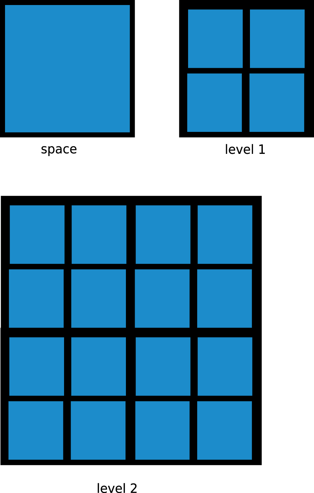
Remark 2.3. The natural fractal structure on [0, 1] ^d is the family of coverings $Δ = {Δ_{n} : n \in ℕ}$ whose levels are defined as $\begin{matrix} Δ_{n} & = & {[\frac{k_{1}}{2^{n}}, \frac{1 + k_{1}}{2^{n}}] \times \dots \times [\frac{k_{d}}{2^{n}}, \frac{1 + k_{d}}{2^{n}}] : \\ k_{1}, \dots, k_{d} = 0, 1, \dots, 2^{n} - 1} \end{matrix}$ for all $n \in ℕ$ (c.f. Fig. 1).

Fig. 1

The figure above illustrates the first two levels in the natural fractal structure on [0, 1] × [0, 1]. Observe that the first level consists of four squares with sides equal to, Γ₂ contains 4² squares with sides equal to $\frac{1}{2^{2}}$ , and in general, level n consists of 4ⁿ squares with sides equal to $\frac{1}{2^{n}}$ .

Interestingly, the following approach becomes especially appropriate to deal with the effective calculation of the box dimension of Euclidean subsets, since it allows applying the already existing procedures to calculate the box dimension of 1-dimensional subsets.

Theorem 2.4.(c.f. Theorem 2.8 in [5]) Let Δ be the natural fractal structure on [0, 1] ^d, and assume that [0, 1] is endowed with the fractal structure Γ whose levels are $Γ_{n} = {[\frac{k}{2^{nd}}, \frac{1 + k}{2^{nd}}] : k = 0, 1, \dots, 2^{nd} - 1}$ . Moreover, let F be a subset of [0, 1] ^d, and α : [0, 1] → [0, 1] ^d a function such that Δ = α (Γ). Then the (lower/upper) box dimension of F equals the (lower/upper) box dimension of α^-1 (F) ⊆ [0, 1] up to a factor, namely, the embedding dimension, d. In particular, if dim_B(F) exists, then dim_B(α^-1 (F)) also exists (and reciprocally), and it holds that $\dim_{B} (F) = d \cdot \dim_{B} (α^{- 1} (F))$ (1)

Alternatively, a more operational version of previous Theorem 2.4 can be stated in the following terms.

Corollary 2.5.(c.f. both Theorem 4.1 and Remark 4.4 in [5]) Let Δ be the natural fractal structure on [0, 1] ^d, and assume that [0, 1] is endowed with the fractal structure Γ with levels $Γ_{n} = {[\frac{k}{2^{nd}}, \frac{1 + k}{2^{nd}}] : k = 0, 1, \dots, 2^{nd} - 1}$ for all $n \in ℕ$ . In addition, let F be a subset of [0, 1] ^d, and α : [0, 1] → [0, 1] ^d a function such that Δ = α (Γ). Then the lower and upper box dimensions of F can be calculated throughout the following expressions, respectively: $\begin{array}{l} {\underline{\dim}}_{B} (F) = d \cdot {\lim_{¯}}_{δ \to 0} \frac{\log N_{δ} (α^{- 1} (F))}{- \log δ} . \\ {\bar{\dim}}_{B} (F) = d \cdot {\lim^{¯}}_{δ \to 0} \frac{\log N_{δ} (α^{- 1} (F))}{- \log δ} . \end{array}$

In particular, if the box dimension of F exists, then $\dim_{B} (F) = d \cdot \lim_{δ \to 0} \frac{\log N_{δ} (α^{- 1} (F))}{- \log δ},$ (2) where $N_{δ} (α^{- 1} (F))$ is the number of δ-cubes that intersect α^-1 (F) ⊆ [0, 1], and a δ-cube in $ℝ^{d}$ is a set of the form $[δ k_{1}, δ (1 + k_{1})] \times \dots \times [δ k_{d}, δ (1 + k_{d})] : k_{1}, \dots, k_{d} \in ℤ$ .

As such, the previous results involve a fractal structure Δ on [0, 1] ^d (i.e., the natural one), another fractal structure Γ on the closed unit interval, and a function α : [0, 1] → [0, 1] ^d such that Δ = α (Γ) to guarantee both Equations (1) and (2). Though there are no restrictions regarding that the α apart from the condition Δ = α (Γ), along upcoming Section 3 we shall highlight an intelligent construction based on a sequence of stages to properly apply Theorem 2.4 (resp. Corollary 2.5) to calculate the box dimension in higher dimensional spaces.

3 The theorem

In this section, we state the key result in this paper. First, we would like to mention that the concept of a starbase fractal structure plays a key role to construct that function α.

Definition 3.1. ([1], Section 2.2) Let Γ be a fractal structure on X. We say that Γ is starbase if $St (x, Γ_{n}) = {St (x, Γ_{n}) : n \in ℕ}$ is a neighborhood base of x for all x ∈ X, where St (x, Γ_n) = ∪ {A ∈ Γ_n : x ∈ A}.

A sequence ${A_{n} : n \in ℕ}$ is said to be decreasing provided that A_n+1 ⊆ A_n for all $n \in ℕ$ .

Definition 3.2. ([2], Definition 3.1.1) Let $Γ = {Γ_{n} : n \in ℕ}$ be a fractal structure on X. We say that Γ is Cantor complete if for each decreasing sequence ${A_{n} : n \in ℕ}$ with A_n ∈ Γ_n, it holds that $\cap_{n \in ℕ} A_{n} \neq \emptyset$ .

Following the concepts above, we have the following

Theorem 3.3. ([4], Theorem 3.6) Let $Γ = {Γ_{n} : n \in ℕ}$ be a starbase fractal structure on a metric space X, $Δ = {Δ_{n} : n \in ℕ}$ a Cantor complete starbase fractal structure on a complete metric space Y, and ${α_{n} : Γ_{n} \to Δ_{n} : n \in ℕ}$ a collection of functions. Consider the following list of statements:

if A∩ B ≠ ∅ with A, B ∈ Γ_n for some $n \in ℕ$ , then α_n (A)∩ α_n (B) ≠ ∅.

If A ⊆ B with A ∈ Γ_n+1 and B ∈ Γ_n for some $n \in ℕ$ , then α_n+1 (A) ⊆ α_n (B).

α_n is onto.

α_n (A) = ∪ {α_n+1 (B) : B ∈ Γ_n+1, B ⊆ A} for all A ∈ Γ_n,

The two following hold for all A ∈ Γ_n and $n \in ℕ$ :

If both conditions (i) and (ii) stand, there exists a unique continuous function α : X → Y such that α (A) ⊆ α_n (A).

If Γ is Cantor complete and conditions (i)–(iv) stand, then α is also onto and we have α (A) = α_n (A).

Proof. Firstly, we shall define the function α : X → Y. For each x ∈ X, there exists a decreasing sequence ${A_{n} : n \in ℕ}$ such that A_n ∈ Γ_n for all $n \in ℕ$ with $x \in \cap_{n \in ℕ} A_{n}$ . Thus, ${α_{n} (A_{n}) : n \in ℕ}$ is also decreasing with α_n (A_n) ∈ Δ_n for all $n \in ℕ$ . Moreover, it holds that ∩_nα_n (A_n) is a single point, since Δ is starbase and Cantor complete. Therefore, we shall define $α (x) = \cap_{n \in ℕ} α_{n} (A_{n})$ . As such, we affirm that α is well-defined. In fact, let x ∈ X and assume that there exist a pair of decreasing sequences of subsets of X, ${A_{n} : n \in ℕ}$ and ${A_{n}^{'} : n \in ℕ}$ , such that $A_{n}, A_{n}^{'} \in Γ_{n}$ for all $n \in ℕ$ with $x \in \cap_{n \in ℕ} A_{n}$ and $x \in \cap_{n \in ℕ} A_{n}^{'}$ , as well. Suppose, in addition, that $\cap_{n \in ℕ} α_{n} (A_{n}) = {y}$ and $\cap_{n \in ℕ} α_{n} (A_{n}^{'}) = {z}$ with y ≠ z. Then there exists a natural number n such that St (y, Δ_n)∩ St (z, Δ_n) = ∅, since Δ is starbase. Hence, $α_{n} (A_{n}) \cap α_{n} (A_{n}^{'}) = \emptyset$ . However, on the other hand, we have that $x \in A_{n} \cap A_{n}^{'}$ for all $n \in ℕ$ . Thus, $α_{n} (A_{n}) \cap α_{n} (A_{n}^{'}) \neq \emptyset$ by condition (i), a contradiction. Accordingly, y = z.

Under both conditions (i) and (ii), the following statements hold:

α (A) ⊆ α_n (A) for all A ∈ Γ_n and $n \in ℕ$ . This is clear from the definition of α.

α is continuous. Let $n \in ℕ$ and x ∈ X. Assume that y ∈ St (x, Γ_n). Then there exists A ∈ Γ_n such that x, y ∈ A. Thus, α (x), α (y) ∈ α (A) ⊆ α_n (A) by condition (3). Hence, α (y) ∈ St (α (x), Δ_n).

α is unique. Let β : X → Y be a continuous function such that β (A) ⊆ α_n (A) for all A ∈ Γ_n and $n \in ℕ$ . Let x ∈ X. Then there exists a decreasing sequence of subsets of X, ${A_{n} : n \in ℕ}$ , such that A_n ∈ Γ_n for all $n \in ℕ$ with $x \in \cap_{n \in ℕ} A_{n}$ , since Γ is starbase and Cantor complete. Hence, $β (x) \in \cap_{n \in ℕ} α_{n} (A_{n}) = {α (x)}$ , so β (x) = α (x) for all x ∈ X.

In addition, assume that Γ is Cantor complete and also that all conditions (i)–(iv) stand. We shall prove that α_n (A) ⊆ α (A) for all A ∈ Γ_n and $n \in ℕ$ , since it implies that α is onto. In fact, let $n \in ℕ, A \in Γ_{n}$ , and y ∈ α_n (A). Let also B_n = α_n (A) and A_n = A. Then by condition (iv), there exists A_n+1 ∈ Γ_n+1 such that A_n+1 ⊆ A_n with y ∈ α_n+1 (A_n+1) ⊆ α_n (A_n). Let B_n+1 = α_n+1 (A_n+1). As such, we can iteratively construct sequences {B_k : k ≥ n} and {A_k : k ≥ n} such that A_k ∈ Γ_k, α_k (A_k) = B_k ∈ Δ_k, y ∈ B_k for k ≥ n, A_n = A, and B_n = α_n (A), as well. Since Γ is starbase and Cantor complete, it holds that ∩_k≥nA_k = {x} for some x ∈ X. Hence, the construction of such sequences leads to y = f (x) with x ∈ A, so y ∈ α (A). □

4 Applications to curve filling

The main goal in this section is to show how Theorem 3.3 allows the construction of space-filling curves with a different nature. As such, while Subsection 4.1 deals with the definition of the Hilbert’s curve by levels, Subsection 4.2 tackles with the construction of a curve filling an attractor. These functions allow defining appropriate connections among the elements in each level of both fractal structures, Γ and gf, and hence, enable the application of Theorem 2.4 (resp., Corollary 2.5) to calculate the box dimension of subsets of $ℝ^{d}$ by means of the box dimension of 1-dimensional subsets.

4.1 A curve filling the Hilbert’s curve

First, let us show how the classical Hilbert’s plane-filling curve (c.f. [10]) can be iteratively described by levels.

Example 4.1. (c.f. Example 1 in [4]) Let (Y, Δ) be a GF-space with Y = [0, 1] × [0, 1] and Δ being the natural fractal structure on [0, 1] × [0, 1] as a Euclidean subset, i.e., $Δ = {Δ_{n} : n \in ℕ}$ , where $Δ_{n} = {[\frac{k_{1}}{2^{n}}, \frac{1 + k_{1}}{2^{n}}] \times [\frac{k_{2}}{2^{n}}, \frac{1 + k_{2}}{2^{n}}] : k_{1}, k_{2} = 0, 1, \dots, 2^{n} - 1}$ for each $n \in ℕ$ . In addition, let (X, ef) be another GF-space where X = [0, 1] and $= {Γ_{n} : n \in ℕ}$ with $Γ_{n} = {[\frac{k}{2^{2 n}}, \frac{1 + k}{2^{2 n}}] : k = 0, 1, \dots, 2^{2 n} - 1}$ . It is worth pointing out that each level n of Γ (resp., of Δ) contains 2²ⁿ elements. Next, we explain how to construct a function α : X → Y such that Δ = α (Γ). To deal with, we shall define the image of each element in level n of Γ through a function α_n : Γ_n → Δ_n. For instance, let $α ([0, \frac{1}{4}]) = {[0, \frac{1}{2}]}^{2}, α ([\frac{1}{4}, \frac{1}{2}]) = [\frac{1}{2}, 1] \times [0, \frac{1}{2}], α ([\frac{1}{2}, \frac{3}{4}]) = {[\frac{1}{2}, 1]}^{2}$ , and $α ([\frac{3}{4}, 1]) = [0, \frac{1}{2}] \times [\frac{1}{2}, 1]$ , as well (c.f. Fig. 2). Thus, the whole level Δ₁ = α (Γ₁) = {α (A) : A ∈ Γ₁} has been defined. It is worth mentioning that this approach provides additional information regarding α as deeper levels of both Γ and Δ are reached via α_n under the two following conditions (c.f. Theorem 3.3):

If A∩ B ≠ ∅ with A, B ∈ Γ_n for some $n \in ℕ$ , then α_n (A)∩ α_n (B) ≠ ∅.

If A ⊆ B with A ∈ Γ_n+1 and B ∈ Γ_n for some $n \in ℕ$ , then α_n+1 (A) ⊆ α_n (B).

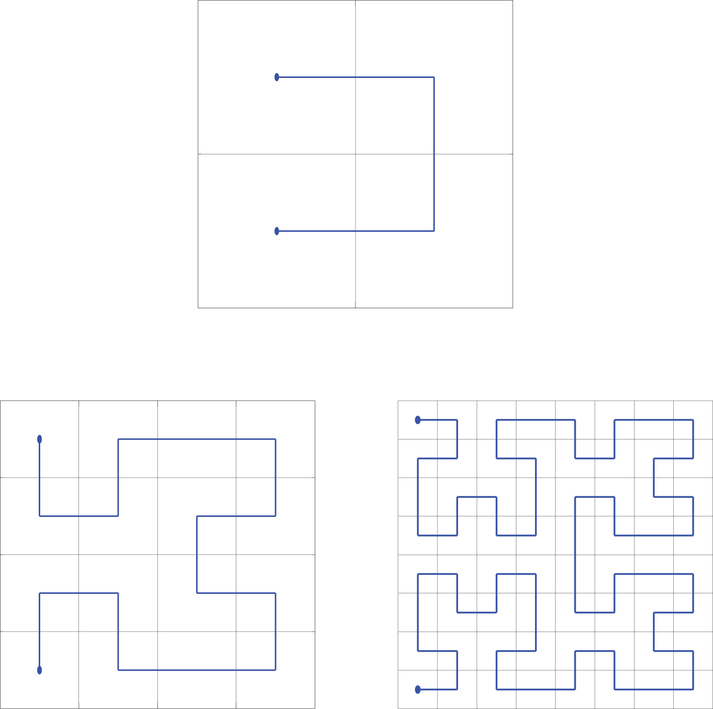
For instance, if A ∈ Γ_n, then we can calculate its image via α_n, α_n (A). Going beyond, let B ∈ Γ_n+1 be so that B ⊆ A. Then α_n+1 (B) ⊆ α_n (A) refines the definition of α_n (A), and so on. This allows us to think of the Hilbert’s curve as the limit of the maps α_n (c.f. Fig. 3). This example illustrates how Theorem 3.3 allows the construction of (continuous) functions and in particular, space-filling curves.

Fig. 2

The two plots above arrange how each element in level n of Γ is sent to some element in level n of Δ via α_n for n = 2, 3.

Fig. 3

First three levels in the construction of the Hilbert’s curve according to Theorem 3.3.

4.2 A curve filling the Sierpinśki gasket

Let k ≥ 2. By an iterated function system, we shall understand a finite collection of similitudes on $ℝ^{d}$ , $ℱ = {f_{1}, \dots, f_{k}}$ , where each self-map $f_{i} : ℝ^{d} \to ℝ^{d}$ satisfies the following identity: $d (f_{i} (x), f_{i} (y)) = c_{i} \cdot d (x, y), for all x, y \in ℝ^{d},$ where d denotes the Euclidean distante and c_i ∈ (0, 1) is the similarity ratio associated with each f_i. Under the previous assumptions, there always exists a unique (nonempty) compact subset $K \subseteq ℝ^{d}$ such that $K = ⋃ {f_{i} (K) : i = 1, \dots, k} .$

The previous equality is usually known as Hutchinson’s equation (c.f. [11]) and $K$ is named the attractor (also the self-similar set) generated by $F$ .

Next, we define the natural fractal structure that each attractor can be always endowed with.

Definition 4.2. (c.f. [3], Definition 4.4) Let $F$ be an IFS whose attractor is $K$ . The natural fractal structure on $K$ as a self-similar set is given by the countable family of coverings $Γ = {Γ_{n} : n \in ℕ}$ , where $Γ_{1} = {f_{i} (K) : i = 1, \dots, k}$ , and Γ_n+1 = {f_i (A) : A ∈ Γ_n, i = 1, …, k} for each $n \in ℕ$ .

It is worth mentioning that such a fractal structure is starbase (c.f. [3, Theorem 4.7]).

Interestingly, it holds that Theorem 3.3 also allows the construction of maps filling a whole attractor. Next, we shall illustrate it by generating a curve that crosses (once) each element of the natural fractal structure which the Sierpiński gasket (c.f. [12]) can be endowed with as a self-similar set (c.f. Definition 4.2).

Example 4.3. (c.f. Example 4 in [4]) Let I = [0, 1] endowed with the fractal structure $Γ = {Γ_{n} : n \in ℕ}$ with levels given by $Γ_{n} = {[\frac{k}{3^{n}}, \frac{1 + k}{3^{n}}] : k = 0, 1, \dots, 3^{n} - 1}$ for each $n \in ℕ$ . In addition, let $K$ be the Sierpiński triangle contained in the equilateral triangle with set of vertices given by ${(0, 0), (\frac{1}{2}, 1), (1, 0)}$ . Let $K$ be endowed with its natural fractal structure as a self-similar set, namely, let $Δ = {Δ_{n} : n \in ℕ}$ with $Δ_{1} = {f_{i} (K) : i \in I}$ and Δ_n+1 = {f_i (A) : A ∈ Δ_n, i ∈ I} for all $n \in ℕ$ , where I = {1, 2, 3} and the three similitudes $f_{i} : ℝ^{2} \to ℝ^{2}$ leading to $K$ are defined as follows: $f_{i} (x, y) = {\begin{array}{l} (\frac{x}{2}, \frac{y}{2}) & if i = 1 \\ f_{1} (x, y) + (\frac{1}{2}, 0) & if i = 2 \\ f_{1} (x, y) + (\frac{1}{4}, \frac{1}{2}) & if i = 3 \end{array}$ for all $(x, y) \in ℝ^{2}$ . Thus, the Sierpiński gasket is fully determined as the unique non-empty compact subset $K$ satisfying the Hutchinson’s equation $K = \cup_{i \in I} f i (K)$ . Observe that each piece $f_{i} (K)$ is a self-similar copy of the whole Sierpiński triangle. Similarly to Example 4.1, next we construct a map γ such that Δ = γ (Γ). Let $n \in ℕ$ . Next, we shall provide further refinements of γ by defining the image of each element A ∈ Γ_n via γ_n : Γ_n → Δ_n. Thus, we can define $γ ([0, \frac{1}{3}])$ as the equilateral triangle whose set of vertices is ${(0, 0), (\frac{1}{2}, 0), (\frac{1}{4}, \frac{1}{2})}, γ ([\frac{1}{3}, \frac{2}{3}])$ , as the equilateral triangle with set of vertices ${(\frac{1}{2}, 0), (\frac{3}{4}, \frac{1}{2}), (1, 0)}$ , and $γ ([\frac{2}{3}, 1])$ is the equilateral triangle with set of vertices ${(\frac{1}{4}, \frac{1}{2}), (\frac{1}{2}, 1), (\frac{3}{4}, \frac{1}{2})}$ , as well. This allows to define Δ₁ = γ (Γ₁) = {γ (A) : A ∈ Γ₁}. Similarly, the next levels of Δ can be defined. Fig. 4 illustrates such a construction. It is worth mentioning that the polygonal line shows the path followed to cross (once) all the elements in each level of the natural fractal structure in $K$ . Thus, $γ = K$ with γ being equal to the limit of the maps γ_n as n→ ∞.

Fig. 4

First two levels in the construction of a curve filling the whole Sierpiński gasket.

Conflict of Interests

The authors declare that there is no conflict of interests regarding the publication of this paper.

Footnotes

Acknowledgments

We thank the reviewers for their constructive comments to improve the quality of this paper. We would like also to thank Prof. M.A. Sánchez-Granero for his insightful remarks concerning this study. He also enabled us the use of both Figs. 1 and .

References

Arenas

F.G.

and Sánchez-Granero

M.A.

, Directed GF-spaces, Applied General Topology2(2) (2001), 191–204.

Arenas

F.G.

and Sánchez-Granero

M.A.

, Completeness in GFspaces, Far East Journal of Mathematical Sciences (FJMS)3(10) (2003), 331–351.

Arenas

F.G.

and Sánchez-Granero

M.A.

, A characterization of self-similar symbolic spaces, Mediterranean Journal of Mathematics9(4) (2012), 709–728.

Fernández-Martínez

and Sánchez-Granero

M.A.

, A new fractal dimension for curves based on frl structures, Topology and its Applications203 (2016), 108–124.

Fernández-Martínez

and Sánchez-Granero

M.A.

, Calculating the fractal dimension in higher dimensional spaces, preprint.

Fernández-Martínez

, A survey on frl dimension for fractal structures, Applied Mathematics and Nonlinear Sciences1(2) (2016), 437–472.

Fernández-Martínez

and Sánchez-Granero

M.A.

, Frl dimension for fractal structures, Topology and its Applications163 (2014), 93–111.

Fernández-Martínez

and Sánchez-Granero

M.A.

, How to calculate the Hausdorff dimension using fractal structures, Applied Mathematics and Computation264 (2015), 116–131.

García

, Mora

and Redtwitz

D.A.

, Box-counting dimension computed by α–dense curves, Fractals25(5) (2017), 1750039 [11 pages].

10.

Hilbert

, Über die stetige Abbildung einer Linie auf ein Flächenstück, Math Ann38 (1891), 459–460.

11.

Hutchinson

J.E.

, Fractals and self-similarity, Indiana University Mathematics Journal30(5) (1981), 713–747.

12.

Sierpiński

, Sur une courbe dont tout point est un point de ramification, C R Math Acad Sci Paris160 (1915), 302–305.

13.

Skubalska-Rafajłowicz

, A new method of estimation of the box-counting dimension of multivariate objects using spacefilling curves, Nonlinear Analysis: Theory, Methods & Applications63(5–7) (2005), e1281–e1287.