An intelligent system to study the fractal dimension of trabecular bones

Abstract

In this paper, we explore the fractal dimension of Cone Beam Computed Tomography images to analyze the trabecular bone structure of healthy subjects. That quantity, computed throughout three distinct approaches, provided us accurate values of normality concerning the radiographic density of this kind of bones and will allow us to establish comparisons with respect to the fractal dimension from patients with different pathologies that may affect the density of trabecular bones.

Keywords

Fractal fractal pattern fractal dimension box-counting dimension fractal structure space-filling curve cone beam computed tomography scan periodontitis bone quality trabecular bone

1 Introduction

Since Dr. Frederic Otto Walkhoff first took a dental radiography in 1896, the radiological field has widely evolved, not only from the viewpoint of the apparatus but also due to the exposure times and the radiation doses. At the same time, William Herbert Rollins built the first dental X-ray unit. However, it was William J. Morton who really used this device, who also contributed to the scientific basis regarding the use of X-rays in the field of dentistry. Several years later, the intraoral radiographic film was used by Dr. Frank Van Woert. In 1913, William D. Coolidge created the first X-ray tube with tungsten filament, a revolution. In 1980, Fred M. Medwedeff, throughout the technique of collimation, managed to reduce exposure significantly. The devices have been improved over the years until the Cone Beam Computed Tomography (CBCT, hereafter) was introduced in 1996 in the European market. Such a method considerably reduces the dose of radiation and exposure and provides high resolution images, as well. In this paper, we have developed a detailed study from high quality CBCT images based on the analysis of their fractal dimensions. Unlike other approaches used in the literature, we have tested a novel approach, completely different from the standard methods usually applied to estimate the fractal dimension in the medical field. We should mention here that the so-called box-counting dimension constitutes the par excellence method to explore fractal patterns in radiographic projections (c.f. [8 –19]).

Next, we highlight two relevant novelties to what has been written so far regarding the present work:

We used CBCT as a unique radiographic study method.

We applied a novel procedure for fractal dimension estimation purposes, supported bytheoretical results, to accurately calculate the box dimension of CBCT images. Interestingly, it throws more accurate results than those obtained by the standard implementation of the box-counting approach. As such, we can specify to what is really happening inside the analyzed bone (c.f. [1]).

It is worth pointing out that the devices we used offered us the possibility of capturing high quality images. This facilitated the application of novel fractal dimension based methods of analysis so sensitive that the results became extremely accurate. In this way, the analyzed CBCT images were captured by the same Planmeca team, Planmeca ProMax 3-D Max (Planmeca Oy, Helsinki, Finland) duly calibrated. Radiographs were taken with the subjects in prone position, adjusting the position of their heads by using the laser guidance system of the device. The beam emission parameters were kV = 96, mA = 8, exposure time of ≃12s, and an image size equal to 501 × 501 × 466 voxels (with each voxel being equivalent to 200 μm). The evaluation software was the Romexis 2.5.1.R (Planmeca Oy, Helsinki, Finland), which allowed observation of the image in a multiple window where the axial, coronal, and sagittal planes can be visualized in 0.2mm intervals, together with a 3D vision. All the subjects taking part in our study were in general and oral health good conditions. They did not present any kind of dental or systemic pathology. They did not take any type of medication that could affect their bone density nor had they taken it in the past. The mean age of the subjects in the sample was 45 years and the same section of the bone, located according to the mental hole in the jaw bone, was analyses in all the cases.

Following the above, the structure of this article is as follows. First, Section 1 provides all the mathematical tools we applied to carry out the present study. More specifically, it contains the basics on the box-counting dimension (box dimension, hereafter) and describes the concept of fractal structure (which our theoretical results are based on). In particular, we define the natural fractal structure on the Euclidean plane. Since we are interested in the calculation of the box dimension for plane CBCT images, all our theoretical development lies in the context of subsets of ^R2. However, it is worth mentioning all of them can be extended to any Euclidean space, if needed. We also provide some theoretical results allowing the calculation of the box dimension of CBCT images in terms of the box dimension of 1-dimensional subsets via a certain function α. Interestingly, a constructive approach to define that function is also contributed at the end of that section. Next, Section 1 is devoted to comment on our computational results. In fact, we explain how the calculations regarding the box dimension of CBCT images have been carried out via three different approaches, namely, the standard box dimension algorithm and two novel approaches based on our theorems, as well. Finally, we provide several remarks to conclude the paper (c.f. Section 1).

2 Mathematical framework

Along this section, we shall provide all the mathematical content we applied to properly study the box dimension of CBCT images. As such, the structure of this section is as follows. In Subsection 2.1, we recall the basics on the box dimension model. Subsection 2.2 contains the foundations on fractal structures and provides the definition of the so-called natural fractal structure which any Euclidean subset can be always endowed with. Subsection 2.3 is devoted to theoretically tackle with the calculation of the box dimension of plane subsets. It is worth pointing out that a pair of results we contribute, namely, Theorem 2.5 and Corollary 2.6, allow the calculation of such a fractal dimension from the box dimension of a 1-dimensional subset. Since such a subset of [0, 1] depends on a function α : [0, 1] → [0, 1] × [0, 1] which relates a fractal structure Γ on [0, 1] with the natural fractal structure on the unit square, Δ, in Subsection 2.4, we provide a constructive approach to properly define it (c.f. Theorem 2.7).

2.1 The box dimension

Next, we recall the concept of box dimension. Its origins go back to the thrities when Pontrjagin and Schnirelman first provided its standard definition (c.f. [7]).

Let δ > 0. By a (plane) δ-cube we shall undertand a set of the form $[δ k_{1}, δ (1 + k_{1})] \times [δ k_{2}, δ (1 + k_{2})] with k_{1}, k_{2} \in ℤ .$ Definition 2.1. Let F be a plane subset. Its lower and upper box dimensions are defined throughout the following asymptotic expressions, resp.: ${\underline{\dim}}_{B} (F) = \underset{δ \to 0}{\lim_{_}} \frac{\log N_{δ} (F)}{- \log δ} .$ ${\bar{\dim}}_{B} (F) = \underset{δ \to 0}{\lim^{¯}} \frac{\log N_{δ} (F)}{- \log δ} .$ In particular, the box dimension of F is given by the following limit (provided that it exists): ${dim}_{B} (F) = lim_{δ \to 0} \frac{log N_{δ} (F)}{- log δ},$ (1) where $N_{δ} (F)$ can be calculated as the number of δ-cubes that intersect F.

The versatility of box dimension lies in the fact that it can be computed with easiness in the context of empirical applications (mainly on Euclidean spaces) involving fractal dimension. In fact, it can be estimated as the slope of the regression line of a graph comparing log δ vs. $log N_{δ} (F)$ plotted over a suitable collection of scales. We shall revisit this fact in forthcoming Remark 3.1.

2.2 Fractal structures

First of all, we recall that a covering of a set X is a collection of subsets, say Γ, such that X = ∪ {A : A ∈ Γ}. The main concept we shall apply along this article for fractal dimension calculation purposes is defined next.

Definition 2.2.[c.f. Definition 2.1 in [5]] Let Γ = {Γ_n : n ∈ ℕ be a countable family of coverings of a given set X. We shall understand that Γ is a fractal structure provided that the two following statements hold:

for each A ∈ Γ_n+1, there exists B ∈ Γ_n such that A ⊆ B.

B = ∪ {A ∈ Γ_n+1 : A ⊆ B} for all B ∈ Γ_n.

It is worth mentioning that covering Γ_n of Γ is called as leveln of that fractal structure. As such, Definition 2.2 states that level n + 1 is a strong refinement of level n of Γ, equivalently. Therefore, if Γ is a fractal structure on X, then we will say that the pair (X, Γ) is a generalized fractal-space (GF-space, for short).

Next, we define what it is understand by the natural fractal structure on the Euclidean plane. It is worth mentioning that such a concept stands as a particular case from Definition 3.1 in [4] or [3] for moredetails.

Definition 2.3. The levels of the natural fractal structure on the Euclidean plane ^R2, Δ = {Δ_n : n ∈ ℕ}, are given by $\begin{matrix} Δ_{n} = {[\frac{k_{1}}{2^{n}}, \frac{1 + k_{1}}{2^{n}}] \times [\frac{k_{2}}{2^{n}}, \frac{1 + k_{2}}{2^{n}}] : k_{1}, k_{2} \in ℤ} \end{matrix}$ for all n ∈ N.

We would like to highlight that the natural fractal structure just defined on ^R2 can be induced on the unit square as follows.

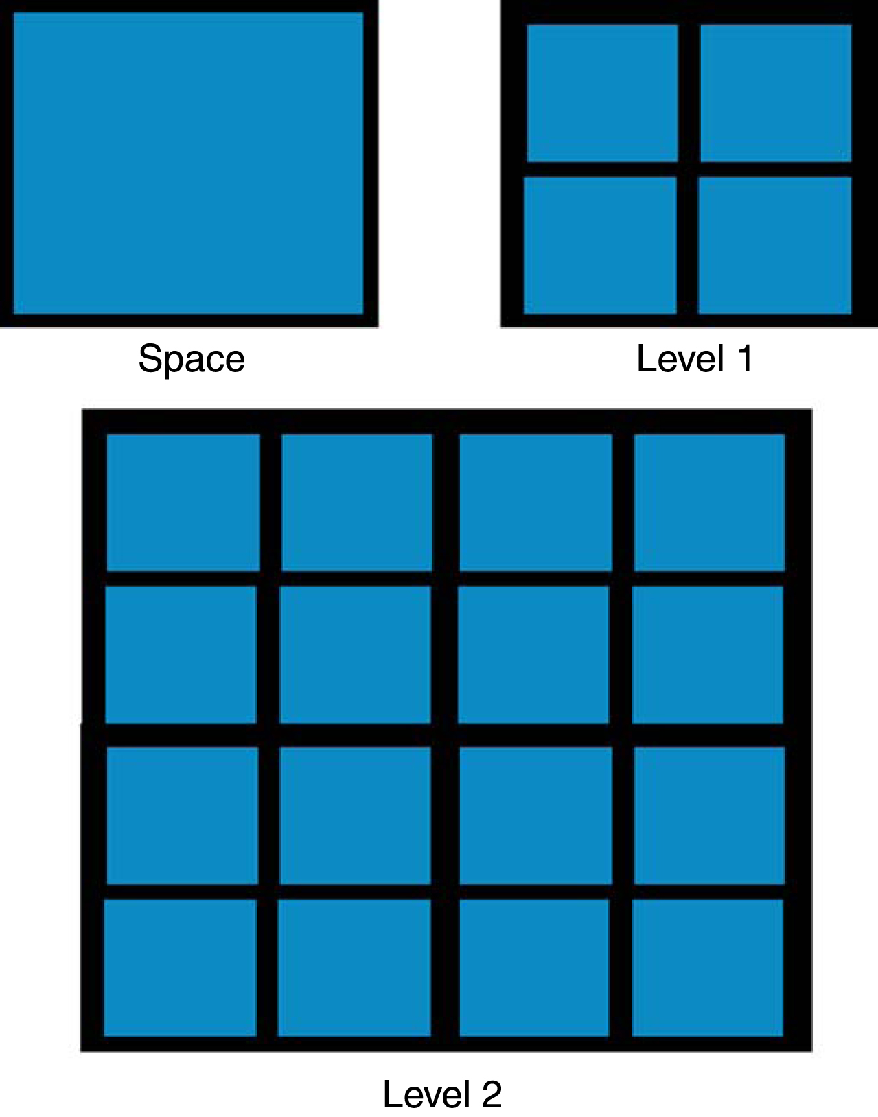
Remark 2.4. The natural fractal structure on the unit square [0, 1] × [0, 1] is the family of coverings Δ= {Δ_n : n ∈ ℕ with levels given by $\begin{matrix} Δ_{n} = & {[\frac{k_{1}}{2^{n}}, \frac{1 + k_{1}}{2^{n}}] \times [\frac{k_{2}}{2^{n}}, \frac{1 + k_{2}}{2^{n}}] : \\ k_{1}, k_{2} = 0, 1, \dots, 2^{n} - 1} \end{matrix}$ for each natural number n (c.f. Fig. 1).

Fig.1

The figure above graphically displays the first two levels in the natural fractal structure on the unit square, [0, 1] × [0, 1]. Observe that the first level consists of four squares with sides equal to, whereas Γ₂ contains 4² squares with sides equal to $\frac{1}{2^{2}}$ . As such, level n would consist of 4ⁿ squares with sides equal to $\frac{1}{2^{n}}$ .

2.3 The calculation of the fractal dimension

The key theoretical result, which supports all the computational calculations carried out along this paper regarding the box dimension of CBCT images (c.f. Section 3), is stated next.

Theorem 2.5. [c.f. Theorem 2.8 in [2]] Let Δ be the natural fractal structure on [0, 1] × [0, 1] and assume that [0, 1] is endowed with the fractal structure Γ with levels given by $Γ_{n} = {[\frac{k}{2^{2 n}}, \frac{1 + k}{2^{2 n}}] : k = 0, 1, \dots, 2^{2 n} - 1}$ for all n ∈ ℕ. In addition, let F be a subset of [0, 1] × [0, 1] and α : [0, 1] → [0, 1] × [0, 1] a function such thatΔ = α (Γ). Then the (lower/upper) box dimension of F equals the double of the (lower/upper) box dimension of α⁻¹ (F) ⊆ [0, 1]. In particular, if bca (F) exists, then bca (α⁻¹ (F)) also exists (and reciprocally), and it holds that $\dim_{B} (F) = 2 \cdot \dim_{B} (α^{- 1} (F)) .$ (2)

Interestingly, as a consequence of Equation (2), we have that the box dimension of each plane subset F (in particular, of each CBCT image we analyzed un upcoming Section 3) equals (up to a constant, namely, the embedding dimension) the box dimension of α⁻¹ (F), a subset of the closed unit interval. It is also worth pointing out that there are no further restrictions regarding the function α : [0, 1] → [0, 1] × [0, 1] apart from the condition Δ= αΓ. Even so, along upcoming subsection, we shall provide the reader a valid procedure to properly construct α.

Next, we state a more operational version of Theorem 2.5 to deal with the effective calculation of the box dimension of plane subsets. As such, we shall highlight that it suffices with calculating the number of δ-cubes that intersect α⁻¹ (F) ⊆ [0, 1] for (lower/upper) bca (F) estimation purposes.

Corollary 2.6. Let Δ be the natural fractal structure on [0, 1] × [0, 1] and assume that [0, 1] is endowed with the fractal structure Γ with levels given by $Γ_{n} = {[\frac{k}{2^{2 n}}, \frac{1 + k}{2^{2 n}}] : k = 0, 1, \dots, 2^{2 n} - 1}$ for all n ∈ ℕ. In addition, let F be a subset of [0, 1] × [0, 1] and α : [0, 1] → [0, 1] × [0, 1] a function such that Δ = α (Γ). Then the lower and upper box dimensions of F can be calculated throughout the following expressions, resp.: ${\underline{dim}}_{B} (F) = 2 \cdot {lim_{_}}_{δ \to 0} \frac{log N_{δ} (α^{- 1} (F))}{- log δ} .$ ${\bar{dim}}_{B} (F) = 2 \cdot {lim^{¯}}_{δ \to 0} \frac{log N_{δ} (α^{- 1} (F))}{- log δ} .$ In particular, if the box dimension of F exists, then $\dim_{B} (F) = 2 \cdot \lim_{δ \to 0} \frac{\log N_{δ} (α^{- 1} (F))}{- \log δ} .$ (3)

2.4 The construction of α

Though Theorem 2.5 gives that the box dimension of F ⊆ [0, 1] × [0, 1] is proportional to the fractal dimension of α⁻¹ (F) ⊆ [0, 1] with α : [0, 1] → [0, 1] × [0, 1] being a function between the GF-spaces ([0, 1], Γ) and ([0, 1] × [0, 1], Δ) so that Δ = αΓ, next we provide a theoretical result allowing a proper construction of α. It is worth pointing out this approach will result useful for box dimension calculation purposes regarding CBCT images (c.f. forthcoming Section 3). Thus, the next result, which involves the fractal structure defined in Remark 2.4, stands from Theorem 3.6 in [6].

Theorem 2.7.Let Γ = {Γ_n : n ∈ ℕ be the fractal structure on [0, 1] with levels given by $Γ_{n} = {[\frac{k}{2^{2 n}}, \frac{1 + k}{2^{2 n}}] : k = 0, 1, \dots, 2^{2 n} - 1}$ , Δ the natural fractal structure on [0, 1] × [0, 1], and α_n : Γ_n → Δ_n a collection of maps. In addition, let us consider the next list of statements:

if A∩ B ≠ ∅ with A, B ∈ Γ_n for some n ∈ N, then α_n (A)∩ α_n (B) ≠ ∅.

If A ⊆ B, where A ∈ Γ_n+1 and B ∈ Γ_n for some n ∈ N, then α_n+1 (A) ⊆ α_n (B).

α_n is onto.

α_n (A) = ∪ {α_n+1 (B) : B ∈ Γ_n+1, B ⊆ A} for all A ∈ Γ_n.

The two following hold:

if α_n satisfies both conditions (i) and (ii), there exists a unique continuous function α : [0, 1] → [0, 1] × [0, 1] so that α (A) ⊆ α_n (A) for each A ∈ Γ_n and all n ∈ N.

Moreover, if (iii)-(iv) also stand for all n ∈ N, then α is onto with α (A) = α_n (A) for all A ∈ Γ_n and each natural number n.

Let us illustrate how previous Theorem 2.7 can be applied to deal with the construction of our function α : [0, 1] → [0, 1] × [0, 1].

Example 2.8.[c.f. Example 1 in [6]] Let us consider the GF-space ([0, 1] × [0, 1], Δ) with Δ being the natural fractal structure on the unit square and let ([0, 1], Γ) be another GF-space with levels given by $Γ_{n} = {[\frac{k}{2^{2 n}}, \frac{1 + k}{2^{2 n}}] : k = 0, 1, \dots, 2^{2 n} - 1}$ . Observe that level n of each fractal structure contains 2²ⁿ elements. Next, we shall explain how to construct a function α : [0, 1] → [0, 1] × [0, 1] such that Δ = αΓ via Theorem 2.7. With this aim, we shall define the image of each element in level n of Γ by a function α_n : Γ_n → Δ_n. Thus, let $α ([0, \frac{14}{]}) = [0, \frac{12}{]} \times [0, \frac{12}{]}, α ([\frac{14}{,} \frac{12}{]}) = [\frac{12}{,} 1] \times [0, \frac{12}{]}, α ([\frac{12}{,} \frac{34}{]}) = [\frac{12}{,} 1] \times [\frac{12}{,} 1]$ , and $α ([\frac{34}{,} 1]) = [0, \frac{12}{]} \times [\frac{12}{,} 1]$ , as well (c.f. Fig. 2). As such, the first level, Δ₁ = α (Γ₁) = {α (A) : A ∈ Γ₁}, is defined. It is worth pointing out that this approach allows refining the definition of α as deeper levels of both fractal structures are reached provided that α_n satisfies both conditions (i) and (ii) in previous Theorem 2. For instance, if A ∈ Γ_n, then we can calculate its image α_n (A). Going beyond, let B ∈ Γ_n+1 be such that B ⊆ A. Then α_n+1 (B) ⊆ α_n (A) refines the definition of α_n (A), and so on. Hence, letting n→ ∞, we can think of the Hilbert’s curve as the limit of the maps α_n (c.f. Fig. 3). This example also highlights how Theorem 2.7 allows the construction of (continuous) functions between (Euclidean) GF-spaces and in particular, space-filling curves.

Fig.2

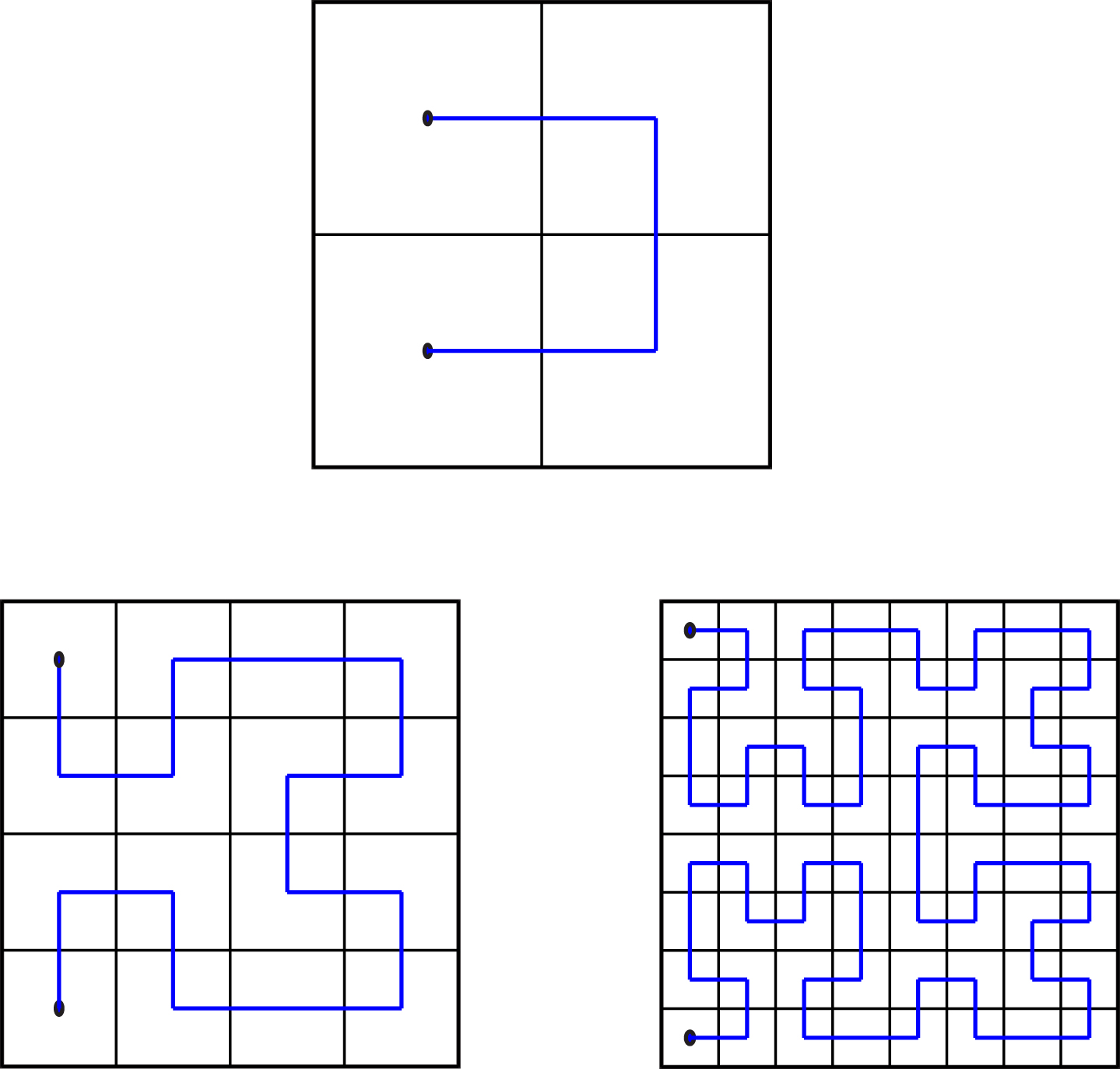
The two plots above arrange how each element in level n of the fractal structure Γ is sent to some element in level n ofΔvia α_n for n = 2, 3.

Fig.3

The figure above displays the first three levels in the construction of the Hilbert’s plane-filling curve according to Theorem 2.7.

3 Computational results

Along this section, we shall carry out some computational experiments regarding the calculation of the box dimension of CBCT images. First of all, we would like to highlight that three different approaches have been applied for box dimension estimation purposes. The first one basically consists of a standard implementation of the box dimension mainly used in computational applications involving fractal dimension. We shall denote it as “Standard box-counting” (SBC, hereafter) approach. It is worth pointing out that the functioning of such a procedure is based on the following expression (c.f. Eq. 1): $\dim_{B} (F) = \lim_{δ \to 0} \frac{\log N_{δ} (F)}{- \log δ},$ where $N_{δ} (F)$ is the number of δ-cubes in [0, 1] × [0, 1] that intersect the given CBCT image, F.

The second procedure tested along this paper deals with the calculation of $N_{δ} (α^{- 1} (F))$ instead of $N_{δ} (F)$ . Observe that $N_{δ} (α^{- 1} (F))$ coincides with the number of elements in each level of the fractal structure Γ that intersect α⁻¹ (F) ⊆ [0, 1]. Recall that level n in such a fractal structure is given by $Γ_{n} = {[\frac{k}{2^{2 n}}, \frac{1 + k}{2^{2 n}}] : k = 0, 1, \dots, 2^{2 n} - 1}$ (c.f. Corollary 2.6). As such, for box dimension estimation purposes, we have applied the following expression: $\dim_{B} (F) = 2 \cdot \lim_{δ \to 0} \frac{\log N_{δ} (α^{- 1} (F))}{- \log δ}$ (c.f. Eq. (1) in Corollary 2.6). We shall denote “box-counting method 1” (BC1, hereafter) that procedure.

Finally, the third algorithm applied herein consists of a slight modification of BC1. It contains several instructions with the aim to improve the calculation of $N_{δ} (α^{- 1} (F))$ . With this aim, they have been considered all the δ-cubes in a given level of Γ that contain at least one pixel of each CBCT image. Let us denote “box-counting method 2” (BC2, for short) this approach.

The next remark becomes necessary to deal with computational applications regarding the calculation of box dimension.

Remark 3.1. Though the box dimension is defined asymptotically provided that the corresponding limit exists (c.f. Eq. (1)), in empirical applications involving box dimension we shall always work by a finite range of scales. It is worth pointing out that, along this paper, we shall consider δ = 2^-n for n = 1, …, 8. Equivalently, fractal patterns will be explored in CBCT images from the first 8 levels of the natural fractal structure on the unit square. This allows us to calculate the slope of the regression line for a plot comparing log n vs. $log N_{2^{- n}} (F)$ , which provides an approach for the box dimension of F. The same arguments remain valid to estimate the box dimension of F via Eq. (1).

Following the above, and for each of the 19 subjects in our sample, we computed the box dimension (by means of each of the three approaches described above) of a pair of CBCT images captured via Romexis 2.5.1.R software: both a 513 × 513 pixel image (low resolution) and a 4364 × 2464 pixel image (original resolution). Fig. 4 has been provided for illustration purposes. It is worth pointing out that all the 19 CBCT images in both resolutions displayed self-similarity patterns in the whole range of 1 - 8 levels analyzed. In fact, all of them displayed linear correlation coefficients quite close to 1 when comparing each scale δ with respect to its corresponding quantity $N_{δ} (F)$ (resp., $N_{δ} (α^{- 1} (F))$ ) for SBC (resp., BC1/BC2) calculation purposes.

The obtained results were as follows. For low resolution images, the mean of the box dimensions of all the subjects was found to be equal to 1.55512 according to SBC with a standard deviation of 0.0578431 (a variance equal to 0.00334583). Regarding BC1, the mean box dimension was equal to 1.95578 and the standard deviation was found to be equal to 0.00627091 (a variance equal to 0.0000393243). On the other hand, BC2 procedure threw the following result: a mean box dimension of 1.9628 and a standard deviation equal to 0.0144581 (a variance equal to 0.000209037). As such, we obtained that both BC1 and BC2 approaches provided similar results in terms of the mean fractal dimension they provided with slight deviations. However, the SBC displayed a different value of the mean box dimension together with a larger deviation than the other methods. Regarding original resolution images, SBC provided a mean box dimension equal to 1.38447 and a standard deviation equal to 0.0758612 (a variance of 0.00575492). On the other hand, BC1 threw a mean fractal dimension equal to 1.98088 with a standard deviation of 0.004269 (a variance equal to 0.0000182244). Similarly, BC2 approach provided a mean box dimension of 1.86931 together with a standard deviation equal to 0.013183 (a variance of 0.000173792). It is worth noting that in this occasion, BC1 and BC2 procedures displayed mean box dimensions not so close among them as in the low resolution case though both of them provided slight deviations with respect to the mean. Again, SBC provided a lower mean box dimension with a larger deviation than the other approaches. It is also worth pointing out that BC2 became more computationally expensive than both SBC and BC1.

Fig.4

The plot above displays a representative CBCT image from a subject of the sample (left figure) as well as an enlargement of a region of the same capture containing a piece of trabecular bone.

4 Concluding remarks

Next, we shall highlight some concluding remarks concerning the study we carried out along this paper.

A priori, each CBCT image possesses a box dimension d with 1 ≤ d ≤ 2. In fact, each picture contains parts of trabecular bone (assumed to display a self-similar structure), so the geometry of such figures lies halfway between a smooth curve (with embedding dimension = 1) and a plane subset (embedding dimension = 2).

Regarding the estimation of the box dimension of such CBCT images, it holds that both approaches BC1 and BC2 behave similarly. However, the results they provided became distinct from those thrown by SBC algorithm.

The functioning of both BC1 and BC2 methods is based on Theorem 2.5 (resp., Corollary 2.6), and in particular, on Eq. (1). In particular, BC2 implements certain instructions to optimise the calculation of $N_{δ} (α^{- 1} (F))$ .

The fractal dimension values obtained via both BC1 and BC2 approaches are refined as higher resolution CBCT images are analyzed. However, the computation time increases, especially in the case of BC2 procedure. Given this, an option may consist of using the low resolution CBCT images to carry out a preliminary analysis regarding the existence of fractal patterns at a first stage. Afterwards, a more accurate study may be performed throughout the high resolution images, if necessary. Even though the fractal dimensions may vary after exploring the high resolution pictures, it is worth noting that they remain uniform along the whole sample with a slight deviation from the mean box dimension.

All the (low and high resolution) CBCT images from the 19 patient sample displayed fractal patterns in the whole range of scales we explored (1 - 8 levels). In fact, in all the cases, a correlation coefficient quite close to 1 was found when comparing δ vs. $N_{δ} (α^{- 1} (F))$ (resp., $N_{δ} (F)$ ) in the case of both BC1 and BC2 approaches (resp., SBC procedure).

It is worth pointing out that for both low and high resolution CBCT images, BC1 provided the lowest deviations from the mean fractal dimension. In this way, we would like to highlight the robustness of both novel algorithms, BC1 and BC2 for box dimension estimation.

Footnotes

Conflict of Interests

The authors declare that there is no conflict of interests regarding the publication of this paper.

Acknowledgments

We thank the reviewers for their constructive comments to improve the quality of this paper. We would like also to thank Prof. M.A. Sánchez-Granero for his insightful remarks concerning this study. He also enabled us the use of bothFigs. 1 and .

References

Fernández-Martínez

, Guerrero Sánchez*

and López Jornet

, A novel approach to improve the accuracy of the box dimension calculations: Applications to trabecular bone quality, To Appear in Discrete and Continuous Dynamical Systems - Series S.

Fernández-Martínez

, Sánchez-Granero

M.A.

Calculating the fractal dimension in higher dimensional spaces, preprint.

Fernández-Martínez

, A survey on fractal dimension for fractal structures, Applied Mathematics and Nonlinear Sciences1(2) (2016), 437–472.

Fernández-Martínez

and Sánchez-Granero

M.A.

, Fractal dimension for fractal structures, Topology and its Applications163 (2014), 93–111.

Fernández-Martínez

and Sánchez-Granero

M.A.

, How to calculate the Hausdorff dimension using fractal structures, Applied Mathematics and Computation264 (2015), 116–131.

Fernández-Martínez

and Sánchez-Granero

M.A.

, A new fractal dimension for curves based on fractal structures, Topology and its Applications203 (2016), 108–124.

Pontrjagin

and Schnirelmann

, Sur une propriété métrique de la dimension, Annals of Mathematics Second Series33(1) (1932), 156–162.

Estrugo-Devesa

, Segura-Egea

, García-Vicente

, Schemel-Suárez

, Blanco-Carrión

, Jané-Salas

and López-López

, Correlation between mandibular bone density and skeletal bone density in a Catalonian postmenopausal population, Oral Surgery, Oral Medicine, Oral Pathology and Oral Radiology, in press.

Jagelavičienė

and Kubilius

, The relationship between general osteoporosis of the organism and periodontal diseases, Medicina (Kaunas)42(8) (2006), 613–618.

10.

Camargo

A.J.

, Arita

E.S.

, Cortéz de Fernández

M.C.

and Watanabe

P.C.A.

, Comparison of two radiological methods for evaluation of bone density in postmenopausal women, International Journal of Morphology33(2) (2015), 732–736.

11.

Law

A.N.

, Bollen

A.-M.

and Chen

S.-K.

, Detecting osteoporosis using dental radiographs: A Comparison of four methods, The Journal of the American Dental Association127(12) (1996), 1734–1742.

12.

Lin

P.L.

, Huang

P.W.

, Huang

P.Y.

and Hsu

H.C.

, Alveolar boneloss area localization in periodontitis radiographs based on threshold segmentation with a hybrid feature fused of intensity and the H-value of fractional Brownian motion model, Computer Methods and Programs in Biomedicine121(3) (2015), 117–126.

13.

Phipps

K.R.

, Chan

B.K.S.

, Madden

T.E.

, Geurs

N.C.

, Reddy

M.S.

, Lewis

C.E.

and Orwoll

E.S.

, Longitudinal study of bone density and periodontal disease in men, Journal of Dental Research86(11) (2007), 1110–1114.

14.

Sener

, Cinarcik

and Baksi

B.G.

, Use of fractal analysis for the discrimination of trabecular changes between individuals with healthy gingiva or moderate periodontitis, Journal of Periodontology86(12) (2015), 1364–1369.

15.

Suer

B.T.

, Yaman

and Buyuksarac

, Correlation of fractal dimension values with implant insertion torque and resonance frequency values at implant recipient sites, International Journal of Oral & Maxillofacial Implants31(1) (2016), 55–62.

16.

Tezal

, Wactawski-Wende

, Grossi

S.G.

, Ho

A.W.

, Dunford

and Genco

R.J.

, The relationship between bone mineral density and periodontitis in postmenopausal women, Journal of Periodontology71(9) (2000), 1492–1498.

17.

Updike

S.X.

and Nowzari

, Fractal analysis of dental radiographs to detect periodontitis-induced trabecular changes, Journal of Periodontal Research43(6) (2008), 658–664.

18.

Yoshihara

, Seida

, Hanada

and Miyazaki

, A longitudinal study of the relationship between periodontal disease and bone mineral density in community-dwelling older adults, Journal of Clinical Periodontology31(8) (2004), 680–684.

19.

Yoshihara

, Seida

, Hanada

, Nakashima

and Miyazaki

, The relationship between bone mineral density and the number of remaining teeth in community-dwelling older adults, Journal of Oral Rehabilitation32(10) (2005), 735–740.