Key point location method for pedestrians in depth images based on deep learning

Abstract

One difficulty that remains in image processing is the accurate location of key points in depth images. This paper presents an intelligent location method for identifying key points in depth images based on deep convolutional neural networks. This study used Kinect to process images, calculating the differences in depth as well as the directional gradient in subject depth images. The entirety of each depth image was traversed through a sliding window to identify the feature vector. Principal component analysis was used to reduce image dimensions. The random forest technique was used to select characteristics of strong classification as well as to actualize training and testing. A depth convolutional neural network was used to detect key points in images of pedestrians. During the study, an experimental test was conducted in a general environment under various conditions, including occlusion and low light. Even under these suboptimal conditions, the detection rate of the proposed method was 87.72%. Furthermore, this method was compared with the GEBCF and FCF algorithms, and proved to increase the detection rate by 0.92% and 0.68%, respectively. Using the depth convolutional neural network in the pedestrian key point positioning experiment, the average error obtained when comparing the predicted point coordinates to the sample mark coordinates was 2.102 pixels. These experimental results show that this method has good accuracy and robustness for the key point location problem of pedestrians in depth images.

Keywords

Pedestrian detection depth image key point location deep learning

1 Introduction

In recent years, associated with the development of high-rise and ultra-high-rise buildings, the public demand for speed and efficiency in many areas has grown. With currently available research, the algorithms used for pedestrian detection primarily include the frame difference, background elimination, and histogram of oriented gradients (HOG) methods. The HOG was proposed by Dalal [1]. This alternative includes feature-based feature extraction, which allows for translation and rotation invariances but still has only limited reductions on the impact of light conversion. When the position of a pedestrian changes, the detection accuracy of this method drops. Reference [2] applied the component model algorithm (DPM), which solved many key problems in this area by detecting human characteristics on different scales. Reference [3] demonstrated a method of calculating the histogram of color features in depth images, as well as implementing recognition and tracking feature matching; comparatively, Reference [4] explored feature extraction from points of interest by detecting these points of interest from video frame depth images. Reference [5] shows a range-sample depth feature for action recognition algorithm that characterizes the distance between points of interest to improve detection results. Most feature extractions based on points of interest display scale and rotation invariance. However, the effects of changes in brightness and weak object texture extraction are low, and as such, the detection accuracy of these methods is low, as demonstrated in Reference [6 –8].

The development of deep learning provides a new method for key point positioning on the human body, as applicable to pedestrians. The deep convolution neural network is one of the most widely used neural network models in deep learning. Applying such deep learning networks to the key point positioning problem has become a hot research area in computer vision. Weight sharing increases the similarities between deep learning and biological neural networks, and when the complexity of the network model and spatial complexity of the model are reduced, the advantages of high-dimensional images become more obvious. Using this method, pictures may be directly input into a deep neural network. This end-to-end structure avoids the processes of complex feature extraction and data reconstruction required in the traditional positioning method. The structure of the deep convolution neural network is suitable for translation, scaling, tilt, or other deformations.

In this paper, a pedestrian detection method based on deep image features is proposed to solve the problems of poor light and occlusion in an elevator waiting hall. This study contributes to the existing literature in three main aspects: (1) it presents a new approach for pedestrian detection based on depth images; (2) it uses a support vector machine based on multiple kernel learning, effectively improving classification accuracy and improving detection accuracy; and (3) the pedestrian detection algorithm, applied in an elevator waiting hall, can forecast the number of passengers on each floor, providing a basis for elevator regulation and effectively improving the efficiency of elevator operation.

2 Depth image feature extraction

The Kinect device used in this study is able to record and input images with unchanged colors and textures as well as solve problems such as blurred contours caused by changes in posture. Kinect is additionally able to eliminate a portion of the impact of backgrounds on the detection process. Since the information stored in the depth images is different from that in conventional color images, the feature extraction method also needs to be altered and improved.

2.1 Depth image preprocessing

A depth image is an image containing distance information from scenes, giving it a stronger anti-interference ability and generally eliminating the influence of changes in illumination and occlusion. However, the Kinect device used in this study captures depth images using an infrared camera, and infrared waves are absorbed by black objects. As such, there will be black holes in these depth images. Reference [9] shows that, when compared to other methods, 8-connected interpolation is best able to fill holes in depth images.

2.2 Depth difference characteristic

Each pixel in a depth image stores corresponding depth information, and a comparison of the differences in depth information between various positions can be used to find the depth difference characteristics (DDC), as shown in Fig. 1. In the depth image (I), the selected pixels (θ₁, θ₂) are in two different positions, while the pixels u₁, u₂ are the offset of θ₁ in the horizontal direction and v₁, v₂ are the offset pixels in the vertical direction. The pixels u₃, u₄, v₃, v₄ are the offsets of θ₂. It can be seen that there exist imparities in depth between the offset pixels in different regions, and also that the differences in depth between closely positioned pixels is small. The depths of the human body and background are very different, and as such the offset pixel depth difference at the edge of the body is notably large relative to the depth differences inside the body. This feature can be used to better extract the edges and internal pixels of a human body.

Fig.1

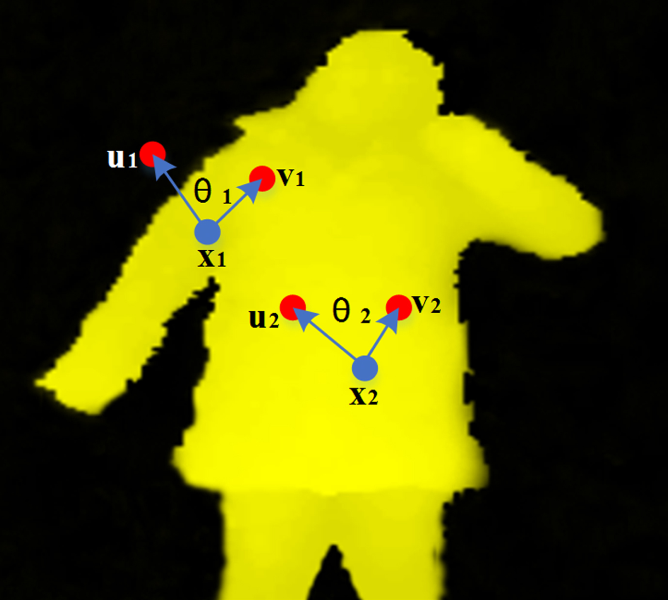
Schematic of depth difference feature.

From this point of view, primary calculations are performed to identify the horizontal and vertical depths of each pixel: $\begin{matrix} Δ_{x} (x, y) = d (x + 1, y) - d (x - 1, y) \\ Δ_{y} (x, y) = d (x, y + 1) - d (x, y - 1) \end{matrix}$ (1)

where d (x, y) is the depth of the pixel located at (x, y) in image I.

Subsequently, the differences in depth in the horizontal and vertical directions (Δ_x, Δ_y) are compared with a threshold value of T_q. When the mean value of Δ_x, Δ_y is less than T_q, the pixel is considered a non-edge point; otherwise, it is an edge point. This threshold value is obtained experimentally. The specific formula for threshold determination is shown in Equation 2: $\begin{matrix} D_{x} = {\begin{matrix} 1, Δ_{x} \geq T_{q} \\ 0, | Δ_{x} | \leq T_{q} \\ - 1, Δ_{x} \leq - T_{q} \end{matrix} & D_{y} = {\begin{matrix} 1, Δ_{y} \geq T_{q} \\ 0, | Δ_{y} | \leq T_{q} \\ - 1, Δ_{y} \leq - T_{q} \end{matrix} \end{matrix}$ (2)

The depth difference characteristic is expressed as: $DDC (x, y) = (D_{x}, D_{y})$ (3)

As such, each image can be represented by a matrix of Equation 3.

2.3 Direction gradient features

The operator of the depth difference feature can be used to better determine the edges of pedestrians, as well as for extracting pedestrians from their background. However, when a portion of the depth differences are small between the background pixels and human body pixels, the two become easily confused. This may result in false detection. The gradient size and direction of each pixel are calculated using the gradient feature of the depth image, which is more accurately able to distinguish between the background and body pixels.

The direction gradient features (DGF) are similar to the histogram of gradient in a color image. First, the gradients in the horizontal and vertical directions are calculated as shown in Equations 4 and 5. $Δ_{x} (x, y) = \frac{d (x + 1, y) - d (x - 1, y)}{2}$ (4) $Δ_{y} (x, y) = \frac{d (x, y + 1) - d (x, y - 1)}{2}$ (5)

where d (x, y) is the depth at pixel (x, y) in image I, and Δ_x, Δ_y are the depth differences in the horizontal and vertical directions.

Sequentially, the gradient vector is transformed into the gradient size and direction, as shown in Equation 6. $\begin{matrix} G (x, y) = \sqrt{Δ_{x} (x, y)^{2} + Δ_{y} (x, y)^{2}} \\ α (x, y) = {tan}^{- 1} (\frac{Δ_{y} (x, y)}{Δ_{x} (x, y)}) \end{matrix}$ (6)

Each pixel in the depth map can thus be represented by its gradient size and direction.

2.4 Feature extraction by sliding window

In order to determine the depth image feature vector, this study uses the HOG algorithm concepts. Primarily, a fixed size detection window is determined and divided into several blocks, as described in Reference [10]. After this, the blocks are divided into several small cell units. The depth differences and direction gradient features of each pixel are calculated in the cells and blocks.

The method of feature extraction is determined following the specific steps, with sizes given for the example used in this study:

First, the depth difference characteristics and direction gradient features of each pixel in the image are calculated;

Second, the image (example, 64×128) to be extracted is divided into a block with a size of 16×16 pixels without overlapping regions, and each block is divided into 2×2 cell units. The space [0°, 360°] is then divided into t bin, with t set to 9 in the example;

The histogram of DDC for all the pixels on the block is then counted to find the 9-dimensional DDC eigenvector for each block.

DDC feature vectors for all blocks are concatenated as “feature one” of the images, with each image consisting of 4×8 blocks and the dimension of image feature one set to 9×4×8 = 288.

The gradient histogram of each cell is calculated with the gradient size as the weight. It is thus possible to obtain the n-dimensional DGF characterization descriptor of each cell unit. The DGF of cell units in all blocks are then linked serially and the eigenvector of the blocks are normalized. The DGF dimension of a block is 2×2×9 = 36.

The step was set to 8 pixels, and when the block is slid across the image there are 7 scanning windows in the horizontal direction and 15 scanning windows in the vertical direction. The DGF feature vector of each block is calculated and the DGF feature vectors of all blocks are connected in series as “feature two” of the image. The dimension of feature two in each image is 36×7×15 = 3780.

The schematic of sliding window is shown in Fig. 2.

Fig.2

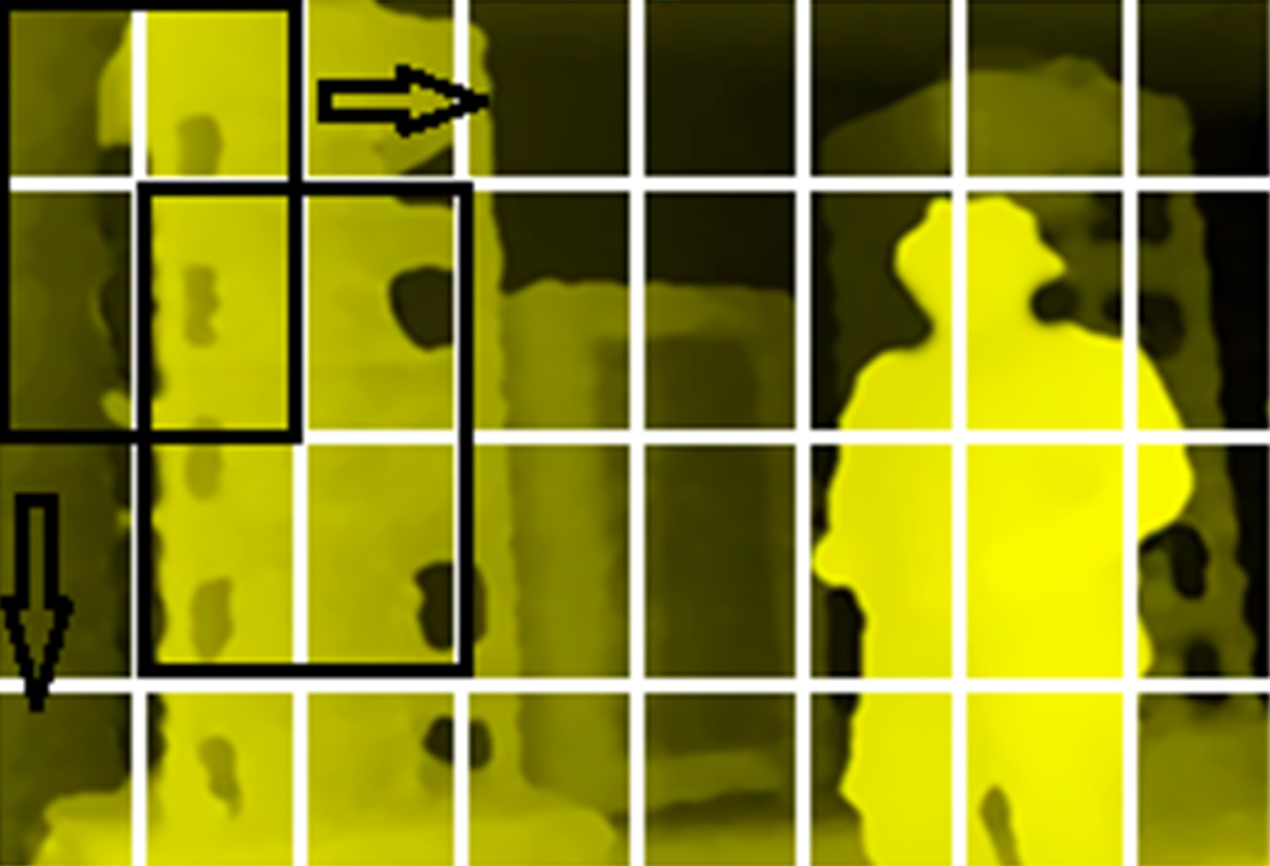
Schematic of feature extraction by sliding window.

2.5 Feature optimization based on principal component analysis

The dimensionality of the directional gradient feature vector is large, which reduces recognition accuracy and also affects the speed of the classification.

These issues make dimensionality reduction very important in the process of feature extraction. It has been found that principal component analysis (PCA) has a significant effect on dimensionality reduction. The PCA algorithm makes spatial transformations through linear transformations of the original variables. This process creates new variables in a lower spatial space, and as the gray scale feature of region shapes in depth images is weak, this dimensionality reduction does not have a significant influence on the expression of the feature. In this study, the PCA method was used to optimize the eigenvector.

PCA optimization is divided into two parts. Firstly, the n-dimensional eigenvector, is obtained when the detection window is optimized. As described in Reference [11], the covariance matrix is constructed using n = σ × δ, where δ = ζ × ζ × β. The mean and covariance matrix formulas are as follows: $μ = \frac{1}{n} \sum_{i = 1}^{n} G_{i},$ (7) $S_{T} = \frac{1}{n} \sum_{i = 1}^{n} (G_{i} - μ) (G_{i} - μ)^{T} = \frac{1}{n} {AA}^{T}$ (8)

where A and G are eigenvector matrices, A ⇔ G and A^T are orthogonal transform matrices, and S_T is a diagonal matrix. The covariance matrix eigenvector is expressed as: $U (i) = \frac{1}{\sqrt{λ (i)}} A χ (i); i = 1, 2, \dots \dots, n$ (9)

where λ (i) is the variance of the eigenvector spatial value and χ (i) is the corresponding eigenvector, as described in Reference [12]. By the principle of the PCA algorithm, these eigenvectors need to be arranged in descending order, and the previous b vectors are selected for operation. The reduced dimension expression is as follows: $V (i) = (G_{i} - u) U (i); i = 1, 2, \dots \dots, p$ (10)

There will be Φ windows in the sliding window detection process, and each window has a corresponding feature sequence in which each sequence feature vector dimension is p, and the constituent number of two-dimensional matrices is Φ × p. Here again the dimension is reduced, and the p vector is taken as the final feature vector of the depth image.

3 Feature fusion and classification

After a feature vector has been extracted to represent the depth of a pedestrian, the classifier is used to generate the model. Common algorithms used for this purpose include the support vector machine (SVM), adaptive enhancement algorithm (Adaboost), neural network algorithm (Neural Networks), and random forest (Random Forest), among other methods. The random forest classifier has good characteristics for fast classification, strong ability, and robustness relative to the alternative algorithms [13].

The random forest classifier is composed of multiple CART decision trees [14]. Each decision tree is trained by sub-samples from the returned samples. The decision tree training process is shown in Fig. 3. A random forest can be constructed from input data via row and column sampling [15]. The specific training process is as follows:

Fig.3

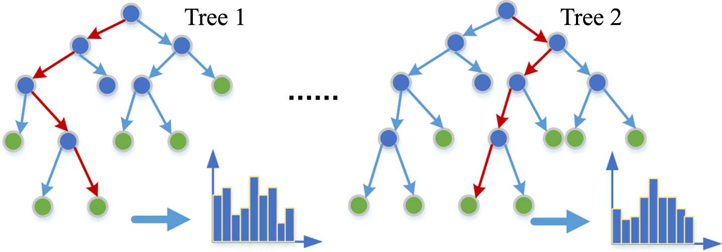
Schematic of t classified using random forest.

In the training sample set S, the bootstrap method is used for sampling (as in Reference [16]), and a sub-training set S_i is generated.

Each subset S generates a decision tree with the following steps:

{1} Select w features from W feature (); where w ≤ W

{2} Select the optimal feature from each of the m features as a splitting feature on each node according to the Gini index ( $Gini = 1 - \sum_{i = 1}^{w} p_{i}^{2}$ );

{3} The completed split is used to establish a decision tree;

{4} Repeat step {2} until all nodes have reached the leaf node or can’t be split;

{5} Repeat steps {1– 3} to form a large number of decision trees, forming a random forest.

4 Deep convolution neural network

The deep convolution neural network is a complex model of convolution layers and sub-sampling layers. The features of sample images are extracted by convolution layer. The sub-sampling layer reduces the number of parameters and weakens the impact of over-fitting on the predicted results. The max-pooling layer is used as a subsampling layer to effectively preserve image features.

In this study, tensorflow was used as the depth learning framework to construct a 10-layer convolution neural network model for accurate positioning training and prediction. The entirety of this convolution neural network model consists of an input layer, an output layer, 4 convolution layers, 4 pool layers and 2 full connect layers. This structure is shown in Fig. 4, and the parameters of the deep convolution neural network are shown in Table 1.

Fig.4

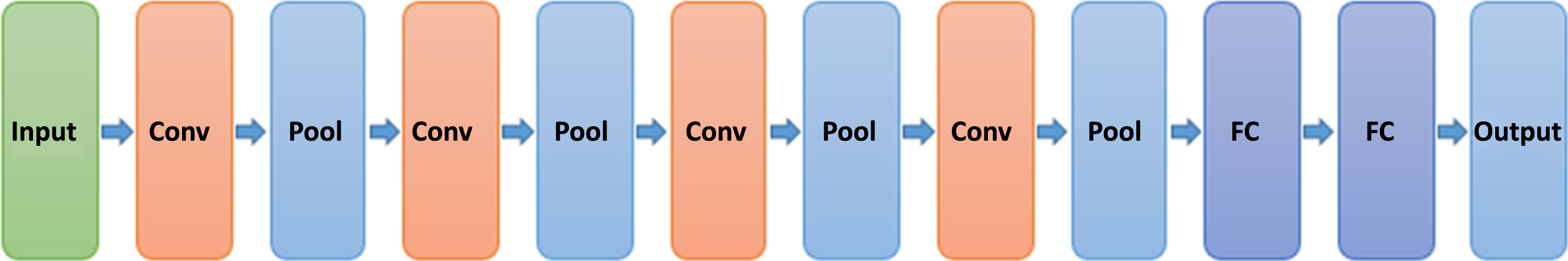
Schematic of deep convolution neural network.

Table 1

Parameters of deep convolution neural network model

Operation	Kernel	Feature maps	Neuron number
448×448 inputs			448×448×3
Convolution	3×3	32	224×224×32
Max pooling	2×2	32	112×112×32
Convolution	3×3	64	56×56×64
Max pooling	2×2	64	28×28×64
Convolution	3×3	128	28×28×128
Max pooling	2×2	128	14×14×128
Convolution	3×3	256	14×14×256
Max pooling	2×2	256	7×7×256
Full connection			1024
Full connection			28

In the deep convolution neural network, a 3×3 convolution kernel was used in the convolution layer, the step was 1, and Rectifier Linear Unit (ReLU) was used as the activation function. ReLU can effectively speed up training and weaken the gradient disappearance phenomenon. The activation function is expressed as follows:

$f (x) = max (0, x)$ (11)

In the deep convolution neural network, the input image is a three-channel color image, and there is also a multi-layer convolution in the hidden layer of the neural network. Thus, a convolution kernel with depth d was introduced in this work. The function is expressed as: $a_{i, j} = f (\sum_{d = 0}^{D - 1} \sum_{m = 0}^{F - 1} \sum_{n = 0}^{F - 1} ω_{d, m, n} x_{d, i + m, j + n} + ω_{b})$ (12)

The depth convolution neural network model proposed in this paper uses the root mean square error between the predicted value and label value as the minimization cost function, and the distance between the predicted value and the label value can be reduced by updating parameters in the neural network to achieve the best result. The loss function can be expressed as: $J = min \sqrt{\frac{\sum_{i = 1}^{n} (X_{obs, i} - X_{label, i})^{2}}{n}}$ (13)

The deep convolution neural network is updated by repeated iterations of a large number of samples. The training process is as follows:

Acquire the image of the candidate frame from the input image and converting it into a grayscale image. Initialize the neural network parameters;

Use the convolution neural network to process this image;

Input the feature vector after dimensionality reduction into to the fully connected layer and map the convolution feature to the coordinate point value;

Obtain the loss value using non-linear regression. The neural network parameters are updated by the Adam optimizer, and the depth convolution neural network model of pedestrian key coordinate values is obtained.

5 Experimental results and analysis

This work was done in the Inter Xeon E5-2630 v3 CPU, NVIDIA GTX 1080 GPU, 16GB memory Ubuntu16.04Lts system, with Python combined OPENCV2.4.8 as a programming experimental platform. The experimental process was conducted in two steps. First, pedestrian detection was conducted using the depth image feature, and then the detected pedestrian image was predicted as the input of the deep convolution neural network model, and obtaining the pedestrian human coordinates.

5.1 Pedestrian detection experiment

Deep image acquisition was performed using the Kinect camera at 30 frames per second. In order to maintain the depth of information, the depth of the image was 16bit and the image gray value range was 0– 65535. When this value is 0, the distance is the most recent effective distance, whereas a value of 65535 represents the longest distance supported by the Kinect camera. In this study, the most effective detection range of the Kinect was between 1.2 and 3.5 m. The sampled depth map is shown in Fig. 5(b).

Fig.5

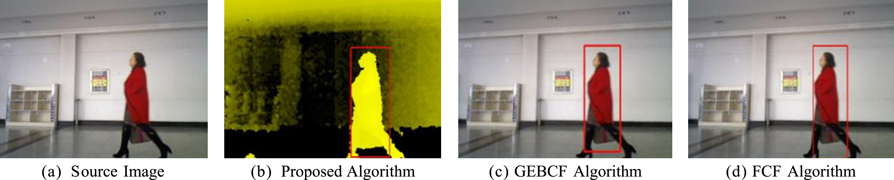
Comparison chart of three detection methods under normal circumstances.

In this study, a comparison test was conducted between three detection methods for pedestrian detection in different scenarios. A representative sample of these test results was selected for display in the experimental results, and the average detection rate of the three methods was calculated including the tests in a general environment, occlusion, weak illumination, and a complex background.

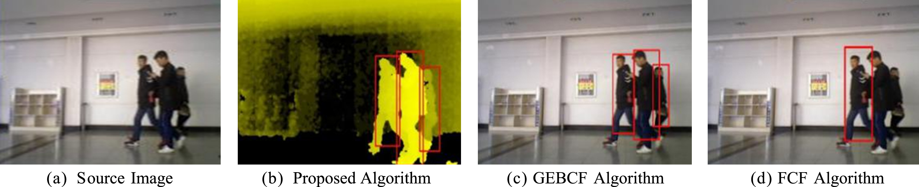
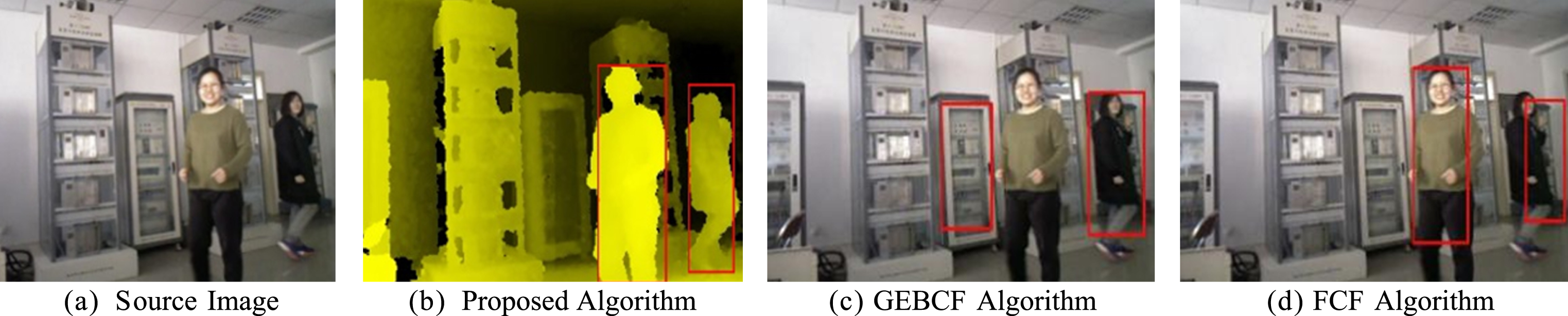
Figure 5 represents the general case portion of the test results, showing that the algorithm has good detection performance in this environment. Figure 8 shows the results of the algorithm (partial detection) when occlusion is present. It can be seen that the proposed algorithm produces better results when occlusion is present, and the detection is more accurate than the other two methods. Figure 7 shows the results of the three algorithms in the case of weak illumination. Figure 8 uses a more complex background for testing detection accuracy.

Table 2 shows the results of the three methods in general, occluded, low-light, and complex background conditions, representing four types of detection rate. Figures 5– 8 graphically represent the experimental results of the three methods under these conditions.

Fig.6

Comparison chart of three detection methods under occlusion.

Fig.7

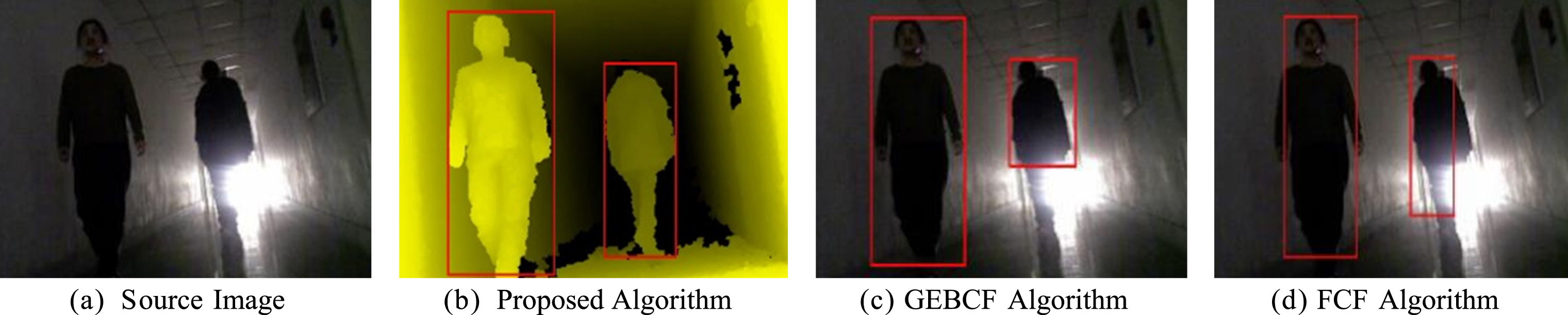
Comparison chart of three detection methods when illumination is weak.

Fig.8

Comparison chart of three detection methods in complex background.

The DET (Detection Error Tradeoff) curve can be used to evaluate the detection of the three methods. The DET curve indicates the relationship between the missed detection and false positive rates.

Table 2

Comparison of detection rates of three methods under different environmental conditions

Environmental Conditions	Detection Rates (%)
	This Study	GEBCF	FCF
Normal circumstances	90.74	91.65	90.23
Occlusion	88.14	87.89	86.39
Weak illumination	84.39	84.52	84.01
Elevator waiting hall	87.69	87.73	86.92

Fig.9

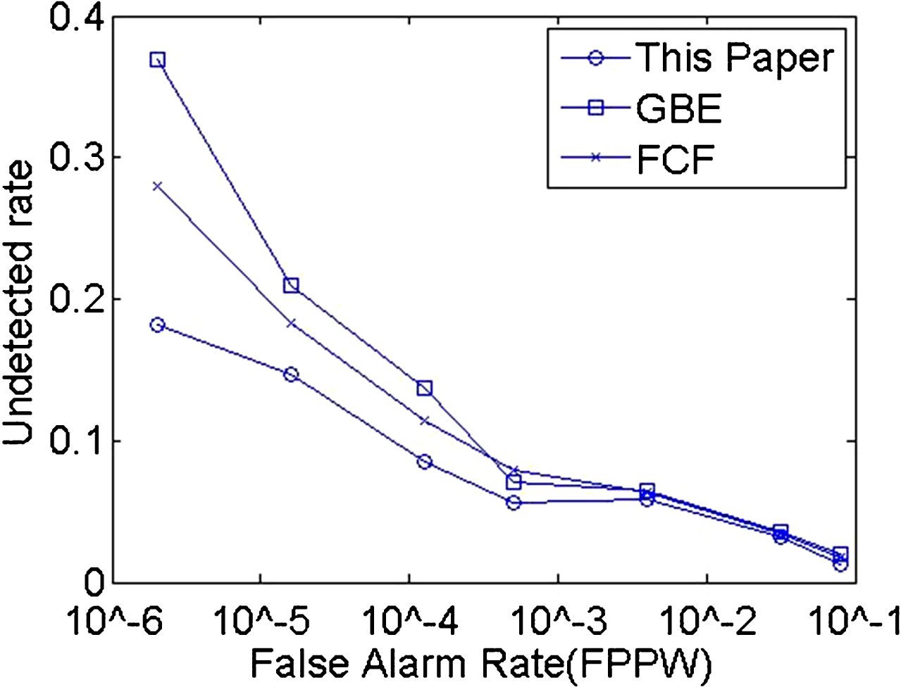
Comparison chart of three DET curve.

It can be seen from Fig. 9 that when the false positive rate is large, the false detection rate of the three algorithms is essentially flat.

However, when the false positive rate is lower than 10^–3, the proposed algorithm has significantly fewer false negative results than the other two. The GEBCF algorithm uses symbiotic characteristics, and in the training process for adding the generalization and detection rate balance link, the detection effect is more stable. However, population density is too large or postural deformation, prone to a sharp decline in the detection rate of the situation. The FCF algorithm filters the underlying features using filter banks and uses boosted decision tree classification to optimize template performance.

However, the influence of external conditions such as illumination is too large in this method. The algorithm proposed in this paper effectively avoids these two issues such that the false test rate in the case of low leakage rates can also be kept low.

5.2 Human key point location experiment

In this study, 1320 pictures were collected and marked, from which 990 were used to generate training samples and 330 pictures were used as test samples. The number of training samples has a distinct impact on the experimental results, and as such enhanced data was used to expand the training samples five times, for a total of 4850 images.

In the training process, the Adam optimizer was used to update the gradient, the learning rate was set to 0.00001, the batch size was set to 32, and Xavier was used to initialize the weights. A total of 2000 training sets were conducted. Figure 10 shows the relationship between the training count and the loss function, where the solid line represents the actual output curve of the loss function and the thick solid line represents the output curve of the loss function average.

In order to solve the problem encountered when the size of a human body image detected using the depth image feature is different, this paper proposes a 0-pixel values filling method. First, the detected human body is cut out to fill the upper left corner coordinate of the box. The pixel values expand pedestrian detection frames of different sizes to 448×448 pixels and enter the convolution neural network for training and prediction. Finally, the predicted pedestrian key points are restored to the original image.

Fig.10

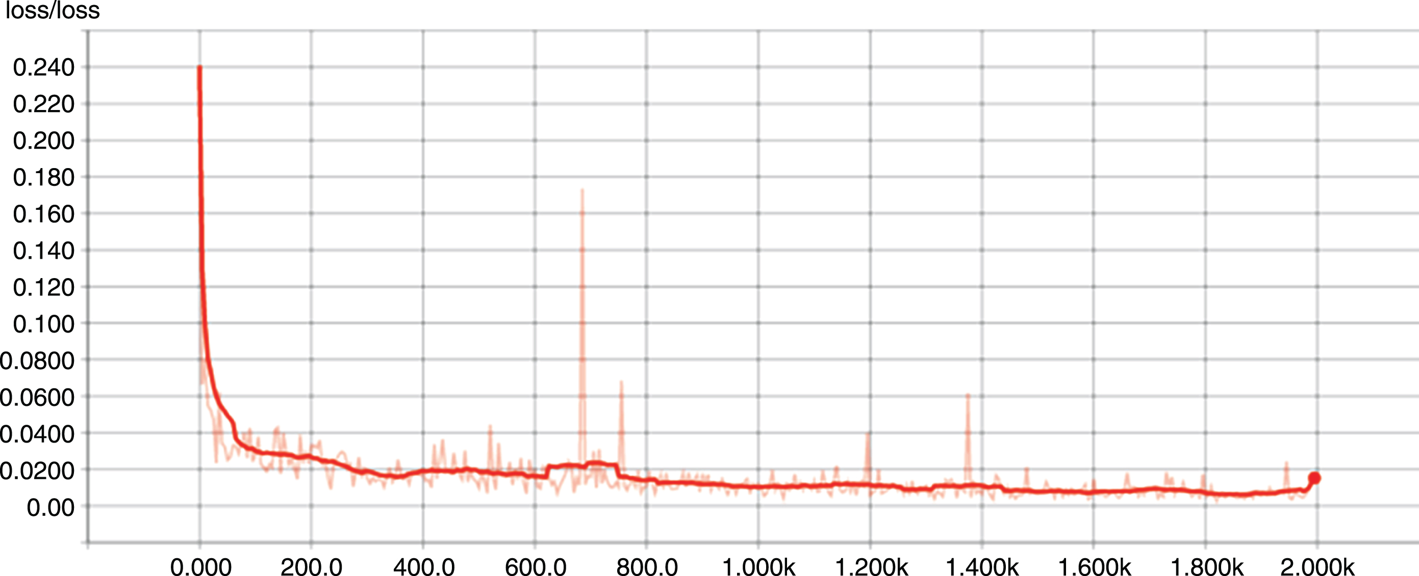
Schematic of loss change.

Figure 11(a) shows the depth feature map, and Fig. 11(b1) and 11(b2) show the results of the experiment based on the results of the pedestrian test and Fig. 11(c1) and 11(c2) shows the 0-pixel values were filled to make the images of the same size. Figure 11(d1) and 11(d2) show the depth of the convolution neural network detection key points, and Fig. 11(e) shows these points reflected in the key points of the human body. After 2000 rounds of training, the depth convolution neural network model was able to predict the coordinates of the coordinate point and sample mark coordinates with an average error of 2.102 pixels. The experimental results show that the proposed method has good accuracy and robustness for human images in different poses and environments.

Fig.11

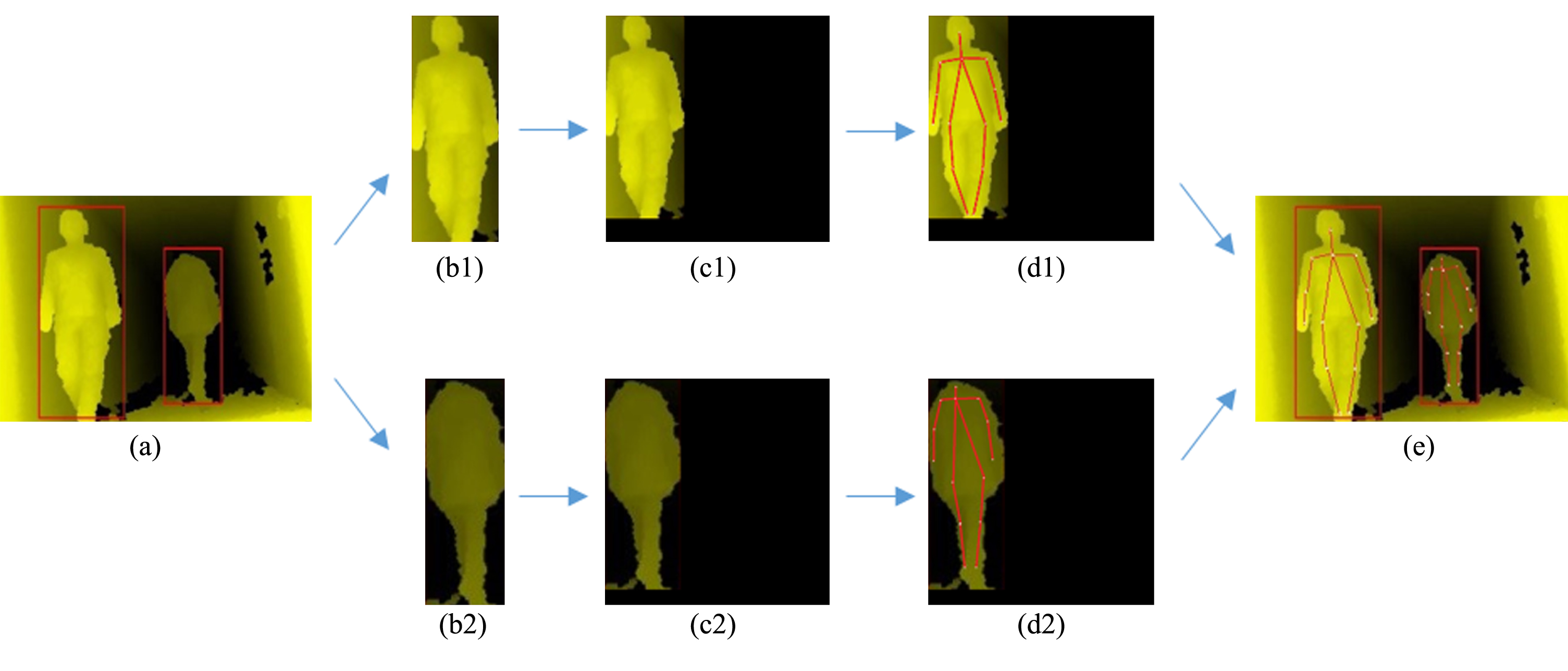
Prediction chart of key points on the human body.

6 Conclusion

Aiming to address the problem of pedestrian detection in buildings, this paper presents a method of depth positioning based on depth learning for depth images containing pedestrians. This research was divided into two parts: pedestrian detection and key point positioning. First, depth information was used to conduct pedestrian detection. A sliding window was used to extract the depth differences and gradient features in the sample depth image. The PCA algorithm was used to reduce the dimension twice in this process, reducing the computational complexity and improving the features and speed of extraction. This matching process can reduce the influence of some external environmental factors on the detection effect of the algorithm, allowing for more accurate determination of pedestrian position information. The key points of detected pedestrians were then positioned to extract the detected human images, and the 0-pixel values were filled into the different sizes of human images to make the images of the same size, and the depth convolution neural network model was established to position the key points of pedestrians. When compared to contemporary pedestrian detection algorithms, this proposed method can improve multi-angle detection accuracy, which is of great significance to solving pedestrian detection and behavior identification in buildings such as airports, car parks, subway stations, and supermarkets.

References

Dalal

and Triggs

, Histograms of Oriented Gradients for Human Detection [C], Computer Vision and Pattern Recognition, 2005 IEEE Computer Society Conference on IEEE, 2005, pp. 886–893.

Felzenszwalb

P.F.

, Girshick

R.B.

, Mcallester

et al.Object detection with discriminatively trained part-based models [J], IEEE Transactions on Pattern Analysis & Machine Intelligence 32 (2010), 1627–1645.

Cui

, Wang

and Liu

, Robust Hand Tracking with Refined CAMShift Based on Combination of Depth and Image Features [C], Robotics and Biomimetics (ROBIO), 2012 IEEE International Conference on IEEE, 2012, pp. 1355–1361.

Karpushin

, Valenzise

and Dufaux

, Local Visual Features Extraction from Texture+Depth Content Based on Depth Image Analysis[C], Image Processing (ICIP), 2014 IEEE International Conference on IEEE, 2014, pp. 2809–2813.

, Jia

and Tang

C.K.

, Range-Sample Depth Feature for Action Recognition [C], Proceedings of the IEEE Conference on Computer Vision and Pattern Recognition, 2014, pp. 772–779.

Shi

P.-B.

, Liu

G.-Q.

and Wang

, Fast incremental learning method for pedestrian detection [J], Journal of Chinese Computer Systems 36 (2015), 1837–1841.

Pedersoli

, Gonzalez

, Hu

et al. Toward real-time pedestrian detection based on a deformable template model[J], IEEE Transactions on Intelligent Transportation Systems 15 (2014), 355–364.

Hinton

and Salakhutdinov

, Reducing the dimensionality of data with neural networks [J], Science 313 (2006), 504–501.

Liu

, Liu

Y.-N.

, Gao

E.-Y.

et al. Human detection method based on foreground segmentation [J], Journal of Chinese Computer Systems 35 (2014), 654–658.

10.

Lee

and Mumford

, Hierarchical Bayesian inference in the visual cortex[J], JOSA A 20 (2003), 1434–1448.

11.

Ren

and Li

Z.N.

, Object Detection Using Generalization and Efficiency Balanced Co-Occurrence Features [C], Proceedings of the IEEE International Conference on Computer Vision, 2015, pp. 46–54.

12.

Zhang

, Benenson

and Schiele

, Filtered Channel Features for Pedestrian Detection [C], Computer Vision and Pattern Recognition (CVPR), 2015 IEEE Conference on IEEE, 2015, pp. 1751–1760.

13.

Yin

H.-P.

, Chen

, Chai

et al. Vision-based object detection and tracking: A review [J], Acta Automatica Sinica 42 (2016), 1466–1489.

14.

Marin

, Vázquez

, López

A.M.

et al. Random Forests of Local Experts for Pedestrian Detection [C], Proceedings of the IEEE International Conference on Computer Vision, 2013, pp. 2592–2599.

15.

Xiang

, Li

X.-D.

et al. Random forests for hierarchical pedestrian detection [J], Application Research of Computers 32 (2015), 2196–2199.

16.

Yang

J.-J.

and Wang

, Application research of discrete orthogonal s-transform in face recognition [J], Journal of Chinese Computer Systems 38 (2017), 169–173.

17.

Warade

, Aghav

, Cladue

et al. Real-Time Detection and Tracking With Kinect [C], 12th IEEE International Conference on Computer and Information Technology Piscataway, USA: IEEE, 2012, pp. 86–89.