Curvature-based sparse rule base generation for fuzzy rule interpolation

Abstract

Fuzzy inference systems have been successfully applied to many real-world applications. Traditional fuzzy inference systems are only applicable to problems with dense rule bases covering the entire problem domains, whilst fuzzy rule interpolation (FRI) works with sparse rule bases that do not cover certain inputs. Thanks to its ability to work with a rule base with less number of rules, FRI approaches have been utilised as a means to reduce system complexity for complex fuzzy models. This is implemented by removing the rules that can be approximated by their neighbours. Most of the existing fuzzy rule base generation and simplification approaches only target dense rule bases for traditional fuzzy inference systems. This paper proposes a new sparse fuzzy rule base generation method to support FRI. In particular, this approach uses curvature values to identify important rules that cannot be accurately approximated by their neighbouring ones for initialising a compact rule base. The initialised rule base is then optimised using an optimisation algorithm by fine-tuning the membership functions of the involved fuzzy sets. Experiments with a simulation model and a real-world application demonstrate the working principle and the actual performance of the proposed system, with results comparable to the traditional methods using rule bases with more rules.

Keywords

Fuzzy inference fuzzy interpolation sparse rule base generation curvature

1. Introduction

Fuzzy sets and fuzzy logic theory provide an efficient way of handling vague information that arises due to the lack of sharp distinctions or boundaries between pieces of information. With the ability to effectively represent and reason human natural language, fuzzy logic theory is considered as an advanced methodology in the field of control systems. The most common fuzzy model is the rule-based fuzzy inference systems, which is mainly composed of two parts: a rule base (or knowledge base) and an inference engine. The inference engines have been defined by different inference approaches, such as the Mamdani model [1] and the TSK model [2]. Although the TSK model is able to generate crisp output, the Mamdani model is more intuitive and suitable for dealing with human natural language. A common feature of all these classical fuzzy inference systems is that they are only applicable to problems with dense rule bases, by which the entire input domain must be fully covered.

Fuzzy rule interpolation (FRI) [3] was initially proposed to address such a limitation due to its ability to work with a spare rule base. When system inputs or observations do not overlap with any rule antecedent values, traditional fuzzy inference systems are not applicable as no rule can be fired. However, fuzzy rule interpolation can still generate a conclusion through a sparse rule base, thereby improving the applicability of fuzzy models. FRI can also be employed to reduce the complexity of complex fuzzy models by excluding those rules that can be approximated by their neighbouring ones. A number of important fuzzy rule interpolation methods have been proposed in the literature, such as [4], which have been successfully applied to deal with real-world problems [8 –14].

Fuzzy rule base generation has been intensively studied in the literature. It is usually implemented in one of two ways: data-driven (extracting rules from data) [15] and knowledge-driven (generating rules from human expert knowledge) [16]. Both approaches may suffer from the ‘curse of dimensionality’. In addition, the knowledge-driven method may be further negatively affected by the limited availability of expert knowledge. Data-driven rule base generation was proposed to minimise the involvement of human expertise. The success of data-driven approaches is built upon a large quantity of training data. These approaches usually only target dense rule bases that are used for traditional fuzzy inference approaches. However, redundancy often exists in fuzzy rule-based models that are acquired from numerical data. This results in unnecessary structural complexity and reduces the interpretability of the system. In order to reduce the complexity of such rule bases, various rule base reduction approaches have been developed to minimise the redundancy [17 –20]. Most of such approaches are based on certain similarity measures; therefore, they are likely to cause performance deterioration along with the size reduction of the rule base.

This paper presents a data-driven rule base generation approach for FRI based on the initial work reported in [21], which directly generates sparse rule bases from data sets by effectively using curvature values traditionally utilised in geography. Different to the conventional fuzzy rule base generation approaches, the proposed approach discriminates rules by calculating their curvature values. Note that curvature values are only workable in three-dimensional spaces (or a rule with two antecedents and one consequence) and thus cannot be directly used for higher-order problems. As a solution, for any given higher-order problem, the proposed approach firstly decomposes the higher-order space into a number of three-dimensional spaces, and then approximates the importance of the higher-order spaces by aggregating the curvature values of the corresponding decomposed three-dimensional ones. From this, the most important rules are selected to form a raw rule base, which is then optimised using a general optimisation approach, such as the genetic algorithm. The proposed approach is validated and evaluated by two experiments; the results demonstrate that the proposed approach is promising.

The rest of the paper is structured as follows. Section 1 Background introduces the theoretical underpinnings of rule base generation, fuzzy rule interpolation, and curvature calculation methods, upon which this work is built. SparseRuleBaseGeneration presents the proposed approach firstly for a basic case with two inputs and then for a general case with multiple inputs. Experimentation details the experimentation for the purpose of demonstration and validation. Conclusion concludes the paper and suggests probable future developments.

2. Background

Background

2.1. Rule base generation and reduction

RuleBase Generation/Reduction Fuzzy modelling describes systems by establishing relations between the relevant variables in the form of if-then rules. There are mainly two types of fuzzy rule base generations for fuzzy modelling. One is knowledge-driven and the other is data-driven. Although early-stage fuzzy models were built by knowledge-driven methods, recently there has been an increasing interest in data-driven methods that can obtain fuzzy models from measured data. According to the different forms of the consequent parts in the if-then rules, there are two types of fuzzy models, Madamni [1] and TSK [2]. A multi-input and single-output (MISO) fuzzy model is represented as a collection of fuzzy rules in the following form: $\begin{matrix} R_{i} : IF x_{1} = A_{i 1} and x_{2} = A_{i 2} and x_{n} = A_{in}, \\ THEN y_{i} = z_{i} (x), \end{matrix}$ (1) where z_i (x) takes different forms depending on the fuzzy models. In the Mamdani model, it is a linguistic label represented by fuzzy sets: z_i (x) = B_i; or in the TSK model, it is often a linear function: $z_{i} (x) = b_{i 0} + \sum_{j = 1}^{s} b_{ij} x_{j}$ .

Most fuzzy rule base generation methods are based on grid-type fuzzy partition. They divide a given problem space into a number of fuzzy regions, each representing a fuzzy rule that is used to construct the final rule base. From this, the raw rule base is optimised by a general optimisation approach, such as the genetic algorithm. As an important benchmark, the method proposed in [15] provides a fast and non-iterative way to learn linguistic rules from data and has been proven with many successful applications [22]. Another successful method is the ‘cooperative rules’ (COR) strategy as reported in [23], which creates a large pool of possible rule-bases using search heuristics.

All these approaches may suffer from the redundancy problem and the ‘curse of dimensionality’. These issues can be addressed by reducing the constructed fuzzy rules through feature selection and instance selection. Empirical studies show that some variables or features are not sufficiently important to be included in the realisation of the fuzzy model during the fuzzy rule base generation process, as some features may be redundant or barely relevant. Thus, the application of feature selection before fuzzy model construction may reduce the fuzzy rule search space and increase the accuracy of the model [24].

2.2. Fuzzy rule interpolation

Fuzzy rule interpolation approaches can be mainly categorised into two classes. The first class directly interpolates rules whose antecedent variables are identical to those observed, with the first FRI technique (referred to as the KH approach) being a typical example [3]. This method is based on the decomposition and resolution principles [25]. According to these principles, each fuzzy set can be represented by a series of α-cuts (α ∈ [0, 1]). Given a certain α, the α-cut of the consequent fuzzy set is calculated from the α-cuts of the observation and from all the fuzzy sets involved in the rules used for interpolation. Knowing the α-cuts of the consequent fuzzy set for all α ∈ [0, 1], the consequent fuzzy set can be assembled by applying the resolution principle. The closed form fuzzy interpolation is another example of this class [6], which can not only be represented in a closed form but also guarantees that the interpolated results are valid fuzzy sets. The stabilised-KH approach extends the original KH approach, which is based on a certain interpolation of a family of distances between fuzzy sets in the rules and in the observation [26]. Unlike the original KH approach, it does not consider the two closest neighbouring rules. Instead, it takes all the rules and computes the conclusion based on the consequent parts weighted by the distances.

The second class of the FRI approaches is based on shape discernibility and an analogical reasoning mechanism, known as ‘analogy-based fuzzy interpolation’ [27]. Instead of directly inferring conclusions, this class works by first creating an intermediate rule such that its antecedent is as ‘close’ to the given observation as possible, given a fuzzy distance metric or other measures based on certain similarity principles. Then, a conclusion is derived from the given observation by firing the generated intermediate rule through an analogical reasoning mechanism. That is, the shape differentiation between the resultant fuzzy set and the consequence of the intermediate rule is analogous to the shape differentiation between the observation and the antecedent of the generated intermediate rule. A number of ways to create an intermediate rule and then to infer a conclusion from the given observation by that rule have been developed, such as the weighted fuzzy interpolative reasoning [7], and the HS approach based on scale and move transformation [4] and its extensions [28, 29]. The HS approaches not only guarantee the uniqueness, normality, and convexity of the interpolated fuzzy sets, but can also handle the interpolation of multiple antecedent variables with different types of fuzzy membership function. They have been extended from different directions, such as adaptive fuzzy rule interpolation [5 , 31], and dynamic fuzzy rule interpolation [32, 33].

2.3. Curvature

CurvatureSection There are two types of methods for curvature calculation. The first type is based on the directional derivative with meshes or curve fitting [34], such as the profile curvature, the streamline curvature, and the planform curvature. The second type is based on a moving least-squares (MLS) surface [35], such as the Gaussian curvature, the mean curvature, the maximum principal curvature, and the minimum principal curvature. The maximum and minimum principal curvatures can be derived from the Gaussian curvature and the mean curvature. The first type is relatively simple and is usually used in meshes or curve fitting situations with more regular data, such as 2D images or maps, and 3D digital elevation models. In comparison, the second type is more complex and is usually used in graphical and engineering applications that contain more irregular discrete data, such as feature recognition, segmentation, and rendering [36].

The first type of curvature calculation methods is based on a directional derivative. A directional derivative represents the steepest downward gradient for a given direction. It refers to the rate at which any given scalar field F(x,y), changes as it moves in the direction of some unit vector, $\hat{n}$ : $D_{(} \hat{n}) (F) = ▽ F \cdot \hat{n},$ (2) where F is a scalar field, $\hat{n}$ is a unit vector. This expression can be used to define several different kinds of curvature calculation, among which the profile curvature is a typical one. It is the rate at which the surface slope, S, changes as it moves in the direction of the unit vector - (▽ f/S), i.e., in Equation 1 Curvature, the scalar field F being S, the unit vector $\hat{n}$ being - (▽ f/S). Note S is the slope defined as the magnitude of the gradient vector: $S (x, y) = | ▽ | = \sqrt{f_{x}^{2} + f_{y}^{2}},$ (3) where the subscripts x and y indicate the partial derivatives of the surface f (x, y), and ▽f is the gradient of this surface.

The profile curvature can also be directly calculated using the partial derivatives with the following formula derived from Equation 2.

V_{P} = \frac{(f_{x}^{2} f_{x x} + 2 f_{x} f_{y} + f_{y}^{2} f_{y y})}{S^{2}} .

(4)

The second type of curvature calculation methods is based on a MLS surface. It defines a MLS surface S as the stationary set of a projection operator ψ_p, i.e., S = {(x ∈ R³| ψ_p (x) = x} . This type of methods explicitly defines the MLS surface as the local minimal of an energy function e(y,a) along the directions given by a vector field n(x). Here, y is a position vector and a is a direction vector. Following this, the MLS surface S can be implied or implemented by determining the vector field n and the energy function e. Suppose a normal vector v_i is assigned to each point of q_i ∈ R³ of an input-point set Q, then the vector field n is: $n (x) = \frac{\sum_{q_{i} \in Q} v_{i} θ (x, q_{i})}{| | \sum_{q_{i} \in Q} v_{i} θ (x, q_{i}) | |},$ (5) where the Gaussian weighting function is defined as: $θ (x, q_{i}) = e^{\frac{- | | x - q_{i} | |^{2}}{h^{2}}},$ (6) where h is a Gaussian scale parameter that determines the width of the Gaussian kernel. If the normal vector v_i is not readily available, as can be the case in some applications, it can easily compute a normal vector for any point with the normalised weighted average of the normals of its nearby sample points. The energy function e: R³ × R³ → R can be defined as: $e (y, n (x_{j})) = \sum_{q_{i} \in Q} ((y - q_{i})^{T} n (x_{j}))^{2} θ (y, q_{i}) .$ (7) It has been proven that the MLS surface is actually an implicit surface function, and the Gaussian or mean curvature can be readily obtained for such implicitly defined MLS surface [37].

It has been proven in [?] that the MLS surface is actually the implicit surface function:

g (x) = n {(x)}^{T} (\frac{δ e (y, n (x))}{δ y} |_{y = x}),

(8)

where n :R³ → R³ is the vector field defined in Equation 5 and e : R³ × R³ → R is the energy function defined in Equation 7. Applying the curvature formulas for implicit surfaces given in [?], the Gaussian and mean curvatures of this implicitly defined MLS surface can be obtained as:

K_{G a u s s i o n} = - \frac{D e t (\begin{matrix} H (g (x)) & \nabla^{T} g (x) \\ \nabla g (x) & 0 \end{matrix})}{{‖ \nabla g (x) ‖}^{4}},

(9)

K_{M e a n} = - (\frac{\nabla g (x) \cdot H (g (x)) \cdot \nabla^{T} g (x)}{{‖ \nabla g (x) ‖}^{3}} - \frac{{‖ \nabla g (x) ‖}^{2} \cdot T r a c e (H)}{{‖ \nabla g (x) ‖}^{4}}),

(10)

Where $\nabla g (x) = {(\frac{\partial g (x)}{\partial x} \frac{\partial g (x)}{\partial y} \frac{\partial g (x)}{\partial z})}^{T}$ is the gradient of g(x), and

H (g (x)) = \nabla (\nabla (g (x))) = {(\begin{matrix} \frac{\partial g (x)}{\partial x \partial x} \frac{\partial g (x)}{\partial x \partial y} \frac{\partial g (x)}{\partial x \partial z} \\ \frac{\partial g (x)}{\partial x \partial y} \frac{\partial g (x)}{\partial y \partial y} \frac{\partial g (x)}{\partial y \partial z} \\ \frac{\partial g (x)}{\partial x \partial z} \frac{\partial g (x)}{\partial y \partial z} \frac{\partial g (x)}{\partial z \partial z} \end{matrix})}^{T}

3. Curvature-based sparse rule base generation

SparseRuleBaseGeneration Curvature is an important concept in the field of geography, which is conventionally used to investigate the water flow over a landscape. Therefore, the curvature values are only workable with three-dimensional spaces. For this reason, the inference problems with two inputs and one output (referred to as the basic case) is considered first, followed by the general case with multiple inputs (referred to as the general case).

3.1. The basic case with two inputs

TheBasicCase By artificially viewing an inference problem (such as classification, diagnosis or prediction) with two inputs and one output as a geometry object, the curvature values as introduced in CurvatureSection can be used to represent the linearity of the object surface. This then reveals the extents to which the geometric object deviates from being ‘flat’ or ‘straight’. Considering that most of the existing FRI approaches are essentially fuzzy extensions of crisp linear interpolation [31], the ‘flat’ or ‘straight’ parts of the geometry object can be easily approximated by its surroundings, and therefore can be omitted. Given a training dataset with two input features and one output feature, the data instances that represent higher curvature values are more important in summarising and generalising the pattern entailed by the dataset. Therefore, they can be used to construct a sparse rule base or to simplify an existing complex rule base. A sparse rule base generation approach based on this motivation for a problem with two inputs and one output is presented below.

3.1.1. Problem domain partition

DomainPartition The partition approaches used in conventional fuzzy rule base generation methods, such as the partitioning and clustering approaches reported in [38], can also be used in this work. Specifically, if the training dataset is sparse, non-grid partition is applied; otherwise, grid partition is used. Given a dataset with two input features (x₁, x₂) and one output feature (y), denote the universe of discourse of the inputs to be [ $\underline{x_{1}}, \bar{x_{1}}$ ], [ $\underline{x_{2}}, \bar{x_{2}}$ ], and that of the output to be [ $\underline{y}, \bar{y}$ ]. If the dataset is very sparse, each data instance in the dataset is used to represent a region. Therefore, the number of regions is equivalent to the number of the data instances in the dataset. If the dataset is dense, the domain is evenly divided into n₁ * n₂ regions. The values of n₁ and n₂ for a given problem are usually empirically determined. Large values of n₁ and n₂ lead to a large rule base, which requires more memory and greater computation efforts. Smaller values of n₁ and n₂ lead to a more compact rule base, which may only offer a poorer performance.

3.1.2. Curvature-based region selection

CurvatureBasedRegionSelection Curvature values represent the ‘straightness’ or ‘flatness’ of a surface, which serves as an important description of intrinsic surface characteristics. Therefore, curvature is intuitively employed as the criterion to select the most important regions and hence to generate the most important rules in the implementation of FRI systems. The curvature value of a region is positively proportional to the importance of the region. A predefined curvature threshold leads to a certain number of rules. Reversely, a predefined rule base size implies a certain curvature threshold. The curvature threshold or the number of rules is problem-specific and usually determined through empirical study.

As discussed in DomainPartition, if the dataset is very sparse, a non-grid partition is applied. The curvature of each partitioned space representing a data instance can be directly calculated using the MLS-based curvature calculation approach as introduced in CurvatureSection. Important data instances can then be selected using either a rule size threshold or curvature value threshold, and the selected important data instances can be directly used for rule base initialisation as introduced in the next subsection.

If a given dataset is dense, grid-partition is used. In order to balance cost and performance, a hierarchical partition and region selection approach is proposed herein to support the rule base generation. The approach is implemented in a recursive manner, and the pseudo-code of the approach is shown in Algorithm 1 hierarchical_partition. In this algorithm, if the curvature value of a region is greater than the activating threshold θ and is less than the ceiling threshold θ * (1 + p), this region will be selected to generate a rule. If the curvature value of the region is less than the threshold θ, the region will be discarded. However, if the curvature value of the region is very large (i.e., larger than θ * (1 + p)), the region cannot accurately be represented by one rule. In this case, this region is further partitioned with the activating threshold θ being updated as θ * (1 + p). Following this, the procedure is recursively applied to each of the further partitioned regions until no region needs to be further partitioned. Note that the curvature threshold is used in this algorithm; the rule size threshold can be applied in a similar and straightforward way, which is thus omitted here.

Algorithm 1 Hierarchical partition &region selection
Inputs:T, the training dataset
n₁, the partition number for input variable x₁
n₂, the partition number for input variable x₂
θ, the curvature threshold
p, a threshold increasing ratio
RR =∅, a set hosts the selected region but
initialised as empty
Outputs:RR, the selected regions
1: ProcedureSelectionT, n₁, n₂, θ, p
2: RR’=GridPartition (T, n₁, n₂)
3: for each R′ in RR′ do
4: if θ ≤ c_R′ ≤ θ * (1 + p) then
5: RR = RR ∪ R′
6: end If
7: ifc_R′ ≥ θ * (1 + p) then
8: Selection(R′, n₁, n₂, θ (1 + p) , p)*
9: end if
10: end for
11: returnRR
12: end procedure

Algorithm 2 Hypercube Selection
Inputs: $ℍ$ : the given set of hypercubes.
m: the required number of rules in the to-be-
generated rule base, ie., the number of selected
data instances.
Outputs: $ℍ^{'}$ : the selected important hypercubes.
1: Procedure HypercubeSelection $ℍ$ , m
2: for each $H_{i} \in ℍ$ do
3: H_i . weight = 0
4: for each C_ij ∈ H_ido
5: H_i . weight ← H_i . weight + v_ij
6: end for
7: end for
8: $ℍ^{″} = {Sort}_{descending} (ℍ)$
9: $ℍ^{'}$ = first m instances in $ℍ^{″}$
10: end procedure

3.1.3. Rule base initialisation

Each selected region is expressed as a fuzzy rule. If the region is led by the non-grid approach, the corresponding data instance is used to represent the region. Denote the fuzzified value of the representative of each region as (A₁, A₂, B); the generated corresponding rule for the region can be expressed as: $If x_{1} = A_{1} and x_{2} = A_{2}, then y = B .$ (11) For simplicity, only isosceles triangular membership functions are utilised in this work. In other words, each fuzzy set A₁, A₂, or B can be defined by a pair (c, s) with c representing the normal point and s representing the support of the fuzzy set, as commonly used in the literature [39]. In this work, the data instance that represents the region is intuitively used to represent the normal point of the triangular membership function, while a fixed support is initially applied to every fuzzy values of a data instance.

If the dataset is dense (and accordingly grid-partition is employed), each region usually covers multiple data instances, and a representative data point is required to represent the region for fuzzy rule generation. This is implemented by firstly aggregating all the data instances into one artificially made data instance, and then such an artificially made data instance is fuzzified using the same approach as discussed above.

A number of ways are available in the implementation of the aggregation operator, such as arithmetic averaging and weighted arithmetic averaging (WAA). The most commonly used approach is WAA, which is also applied in this work. This approach first weights all the given arguments, and then aggregates all these weighted arguments into a collective one. For simplicity, as the curvature values of the data instances already imply their importance, the curvature values are intuitively employed as a means to rank their weights in the WAA method. Suppose a given region is formed by n data instances, the artificially made data instance representing the selected region can be calculated as follows: $c = WAA (a_{1}, a_{2}, . . ., a_{n}) = \sum_{i = 1}^{n} w_{i} a_{i},$ (12) where a_i (1 ≤ i ≤ n) represents the ith data instance included in the selected region, and w_i indicates the weight of a_i: $w_{i} = \frac{C_{i}}{\sum_{i = 1}^{n} C_{i}},$ (13) where C_i represents the curvature value of data instance a_i.

3.2. General case with multiple inputs

TheGeneraralCase

The majority of real-world applications consists of more than two inputs. Thus, the approach proposed in the last section needs to be extended. Given that traditional curvature values only work with three-dimensional data, the most challenging part to evaluate the importance of a high-dimensional instance is that there is no exiting approach to be directly applied for calculating the ‘curvature’ value of a high-dimensional instance. However, a higher-dimensional complex problem can be regarded as a collection of three dimensional problems with two inputs and one output (i.e., multiple basic cases). With the curvature-based approach discussed in TheBasicCase, any high-dimensional problems can thus be addressed by applying the basic case solutions multiple times.

3.2.1. Problem domain partition

ProblemDomainPartion3 Suppose that a complex problem P_n+1 (n > 2) contains n input features $𝕏 = {x_{1}, x_{2}, \dots, x_{n}}$ and one output feature y, and that the universe of discourse of the input features is [ $\underline{x_{1}}, \bar{x_{1}}$ ], [ $\underline{x_{2}}, \bar{x_{2}}$ ],…, [ $\underline{x_{n}}, \bar{x_{n}}$ ], whilst that of the output is [ $\underline{y}, \bar{y}$ ]. Similar to the problem domain partition for the basic cases, each data instance in the dataset represents a hypercube in the problem domain. Therefore, the number of hypercubes will be equivalent to the number of the data instances in the dataset if the dataset is very sparse. In this case, each hypercube is represented as a fuzzy rule.

If the dataset is dense, grid partition is applied. In this situation, the input domain is evenly partitioned into m₁ * m₂ * . . . * m_n hypercubes, where m_i, 1 ≤ i ≤ n, represents the number of partitions in the variable domain of x_i. The values of m_i are usually empirically determined by experts or statistically calculated by clustering methods such as k-means. Traditional fuzzy partition methods represent each hypercube as a fuzzy rule. Hence, any given complex problem P_n+1 will lead to a rule base with m₁ * m₂ * . . . * m_n fuzzy rules [40].

For simplicity, let h be the number of data instances if the given dataset is sparse, and h = m₁ * m₂ * . . . * m_n if the given dataset is dense. Accordingly, the generated hypercubes can be collectively represented as $ℍ = {H_{1}, H_{2}, \dots, H_{h}}$ . Note that some of these rules may not be necessary or can be represented by their neighbouring ones. Therefore, the importance of the hypercubes needs to be discriminated such that a sparse rule base can be generated based on the most significant hypercubes.

3.2.2. Representing hypercube in cubes

The traditional curvature value is only applicable in a geometric space with three dimensions. Hence, there is no equation to directly calculate a ‘curvature’ value for a high-dimensional instance, and thus to directly use the value for representing its importance. However, based on the curvature values of its decomposed cubes, the importance of a high dimensional hypercube can still, to some extent, be identified. In order to distinguish important hypercubes, every high-dimensional hypercube H_i, 1 ≤ i ≤ h, is broken down into $c = C_{n}^{2} = \frac{n!}{2! (n - 2)!}$ cubes. This is done by considering all the combination of two input features and the output feature. Therefore, the collection of hypercubes and the corresponding decomposed cubes can be represented as: $ℍ = (\begin{matrix} H_{1}, H_{2}, \dots, H_{h} \end{matrix}) = (\begin{matrix} C_{11} & C_{21} & C_{31} & \dots & C_{h 1} \\ C_{12} & C_{22} & C_{32} & \dots & C_{h 2} \\ ⋮ & ⋮ & ⋮ & ⋮ & ⋮ \\ C_{1 c} & C_{2 c} & C_{3 c} & \dots & C_{hc} \end{matrix}),$ (14) where C_ij represents the jth cube of the ith hypercube H_i, 1 ≤ i ≤ h and 1 ≤ j ≤ c. Note that cubes C_1j, C_2j, ⋯, C_hj share the same two input features for any 1 ≤ j ≤ c.

The importance of a hypercube can be collectively determined by its decomposed cubes. That is, the importance of hypercube H_i can be determined by the curvature values of C_i1, C_i2, ⋯ , C_ic. The curvature value v_ij of each artificially created cube C_ij can be calculated using the approach detailed in CurvatureSection. Collectively denoting the values of all cubes as V, the calculated results of all cubes can then be represented as follows: $V = (\begin{matrix} v_{11} & v_{21} & v_{31} & \dots & v_{h 1} \\ v_{12} & v_{22} & v_{32} & \dots & v_{h 2} \\ ⋮ & ⋮ & ⋮ & ⋮ & ⋮ \\ v_{1 c} & v_{2 c} & v_{3 c} & \dots & v_{hc} \end{matrix}) .$ (15)

3.2.3. Hypercube selection

The importance of each hypercube can be represented by the summation of the curvature values of its decomposed cubes. In particular, given a set of hypercubes $ℍ$ and the required number of rules m in the to-be-generated rule base or an accumulated curvature threshold θ, the algorithm selects a set of the significant hypercubes as the output $ℍ^{'}$ , using a way similar to the approach presented in CurvatureBasedRegionSelection. Note that if the parameter θ is given, the algorithm works on the same principle as Algorithm2 hierarchical_partition; thus, the details are omitted here.

If the parameter m is given instead of using θ, the hypercube selection process is summarised in Algorithm 3 hypercubeselection. The most significant m instances or hypercubes can be selected simply by taking the first m hypercubes with the highest accumulated curvature values after ranking them in descending order, as expressed in Line 8. The accumulated curvature value regarding a hyper cube H_i, represented as H_i . weight, can be calculated as the summation of all its related decomposed cubes (as expressed in Line 5).

Algorithm 3 Feature Discrimination
Inputs: $ℍ^{'}$ : the selected set of hypercubes.
b: the number of selected input features.
T: the training dataset.
Outputs: $𝕏^{'}$ : a set of the significant features.
1: procedureFeatureDiscrimination( $ℍ^{'}, b, T$ )
2: $ℝ = \emptyset$
3:forj = 1 → cdo
4: Generate an artificial rule base R_j
using all cubes C_ij
5: $ℝ = ℝ \cup R_{j}$
6: p_j=FRI(T, R_j)
7:end for
8: $ℝ^{'} = {Sort}_{Ascending} (ℝ, p_{j})$
9:for $R_{j} \in ℝ^{'}$ do
10: $R_{j} . weight \leftarrow CalculateWeight (ℝ^{'}, R_{j})$
11:end for
12:for each input dimension $x_{k} \in 𝕏$ do
13: x_k . weight* ← 0*
14: for each $R_{j} \in ℝ^{'}$ do
15:ifx_k is used by R_jthen
16:x_k . weight ← x_k . weight + R_j . weight
17: end if
18: end for
19: end for
20: ${Sort}_{Ascending} (𝕏$ )
21: $𝕏^{'}$ = first b features in $𝕏$
22: end procedure

3.2.4. Feature discrimination

In addition to the fact that some hypercubes are more important than the others, some dimensions in a selected hypercube may also be more significant than the others. Therefore, selective dimensionally reduced hypercubes can be used to generate a more compact rule base with fewer rule antecedents. This is summarised in Algorithm 3 featurediscrimination. It takes the output of HypercubeSelection () as its input, in addition to the number of selected features b and the training data T. The output of the algorithm is a subset of input features $𝕏^{'}$ , which represent the most significant input features from the entire set of input features $𝕏$ .

The algorithm artificially generates c set of two-input and one-output fuzzy rule bases to evaluate the importance of the pair of associated features. Recall that since C_1j, C_2j, ⋯ C_hj share the same input features in Equation CurvatureRankingofCubes, they jointly form the jth artificial rule base. Every pair of input features is then evaluated by its corresponding rule bases by applying the training dataset to perform FRI with the rule bases. From this, all the artificial rule bases, representing every pair of features, can be ranked. A weight function is designed to convert the ranking to a weight for the pair of features. Note that each input feature appears in $| 𝕏 - 1 |$ artificial rule bases. Therefore, the importance of the feature is calculated as the summation of the weights of all the rule bases that consider such feature.

3.2.5. Rule base initialisation

Similar to the basic case, each hypercube with selected features is expressed as a fuzzy rule. Denote the fuzzified values of a data instance or a hypercube with b selected input features and the output feature as (A_k1, A_k2,. . . A_kb, B_k); the corresponding fuzzy rule can be expressed as: $\begin{matrix} If x_{1} = A_{k 1}, x_{2} = A_{k 2}, \dots, and x_{b} = A_{kb}, \\ then y = B_{k} . \end{matrix}$ (16)

Note that the above rule base is a Mamdani-style rule base, as the consequence of each rule is a fuzzy set [41]. However, depending on the real-world application, a TSK-style rule base may also readily be generated using the existing TSK rule base generation approaches [42]. Note that the resultant rule base has only b antecedents, which is a subset of the input features. In an extreme situation, the resultant rule base may only have two input features, which backtracks to the basic case as discussed in TheBasicCase.

3.3. Rule base optimisation

Optimisation The initialised rule base can be improved by fine-tuning the involved fuzzy sets, given that the initialised fuzzy sets are specified based on empirical knowledge. This can be implemented using any general optimisation approaches; the genetic algorithm (GA) is particularly employed in this work due to its effectiveness in rule base optimisation [43]. Specifically, a chromosome is designed to represent all the fuzzy sets in the initialised rule base. Given the fixed representative value and isosceles shape of a fuzzy set A, its membership function can be readily constructed from the support of A (denoted as S (A)). Then, each rule with b antecedents and one consequent can be represented by b + 1 parameters: S (A_i1), S (A_i2),…, S (A_ib), and S (B_i). Thus, a chromosome representing all the rules in the rule base has (b + 1) * m genes, where m represents the number of rules in the rule base.

Following this, the initial population can then be generated by creating a number of individuals, i.e., $ℙ = {I_{1}, I_{2}, . . ., I_{| ℙ |}}$ . Each individual I_i is a chromosome representing a potential solution to the given problem, where $1 \leq i \leq | ℙ |$ . Two genetic operations (crossover and mutation) are used to produce the next generation of the population. An objective function is designed to measure the fitness or quality of the individuals, with the root mean squire error (RMSE) used in this work. After this, a number of the best individuals in the next generation are selected and used to replace the worst-ranked individuals in the initial population. In this way, one iteration of the GA process is completed. This process is iterated until the pre-specified maximum number of iterations is reached or the objective value of an individual is less than a predefined threshold. When the GA terminates, the fittest individual in the current population is the optimal solution.

4. Experimentation

Experimentation The proposed method was evaluated using a synthetic dataset and a real-world application, i.e., an indoor environment localisation problem. The first experiment demonstrates the working procedure of the proposed approach, whilst the second one shows the power of the proposed approach in solving real-world problems. The program was developed using Matlab (R2017b) and was run on a laptop with the Intel i7-4810MQ CPU 2.8 GHz and 16 GB of RAM, on Windows 7.

Table 1
The initialised rule base for Experiment 1

	IF		THEN		IF		THEN
i	x	y	z	i	x	y	z
1	(-5, - 4.5, - 4)	(-5, - 4.5, - 4)	(0.881, 0.981, 1.081)	13	(0, 0.5, 1)	(-1, - 0.5, 0)	(-0.125, - 0.025, 0.075)
2	(-5, - 4.5, - 4)	(4, 4.5, 5)	(-1.081, - 0.981, - 0.881)	14	(-1, - 0.5, 0)	(0, 0.5, 1)	(-0.125, - 0.025, 0.075)
3	(4, 4.5, 5)	(-5, - 4.5, - 4)	(-1.081, - 0.981, - 0.881)	15	(0, 0.5, 1)	(0, 0.5, 1)	(-0.075, 0.025, 0.125)
4	(4, 4.5, 5)	(4, 4.5, 5)	(0.881, 0.981, 1.081)	16	(-1, - 0.5, 0)	(-1, - 0.5, 0)	(-0.075, 0.025, 0.125)
5	(4, 4.5, 5)	(5, 5.5, 6)	(0.874, 0.974, 1.074)	17	(5, 5.5, 6)	(-6, - 5.5, - 5)	(-1.068, - 0.968, - 0.868)
6	(4, 4.5, 5)	(-6, - 5.5, - 5)	(-1.074, - 0.974, - 0.874)	18	(-6, - 5.5, - 5)	(-6, - 5.5, - 5)	(0.868, 0.968, 1.068)
7	(-6, - 5.5, - 5)	(4, 4.5, 5)	(-1.074, - 0.974, - 0.874)	19	(-6, - 5.5, - 5)	(5, 5.5, 6)	(-1.068, - 0.968, - 0.868)
8	(-5, - 4.5, - 4)	(4, 4.5, 5)	(0.874, 0.974, 1.074)	20	(5, 5.5, 6)	(5, 5.5, 6)	(0.868, 0.968, 1.068)
9	(5, 5.5, 6)	(4, 4.5, 5)	(0.874, 0.974, 1.074)	21	(-5, - 4.5, - 4)	(-4, - 3.5, - 3)	(0.789, 0.889, 0.989)
10	(-5, - 4.5, - 4)	(5, 5.5, 6)	(-1.074, - 0.974, - 0.874)	22	(4, 4.5, 5)	(-4, - 3.5, - 3)	(-0.989, - 0.889, - 0.789)
11	(5, 5.5, 6)	(-5, - 4.5, - 4)	(-1.074, - 0.974, - 0.874)	23	(-4, - 3.5, - 3)	(4, 4.5, 5)	(-0.989, - 0.889, - 0.789)
12	(-6, - 5.5, - 5)	(-5, - 4.5, - 4)	(0.874, 0.974, 1.074)

Table 2

The optimised rule base for Experiment 1

	IF		THEN		IF		THEN
i	x	y	z	i	x	y	z
1	(-4.999, - 4.5, - 4.001)	(-4.999, - 4.5, - 4.001)	(0.962, 0.981, 1)	13	(-2.192, 0.5, 3.192)	(-2.456, - 0.5, 1.456)	(-0.303, - 0.025, 0.253)
2	(-4.999, - 4.5, - 4.001)	(3.998, 4.5, 5.002)	(-1, - 0.981, - 0.962)	14	(-2.149, - 0.5, 1.149)	(-2.275, 0.5, 3.275)	(-0.273, 0.025, 0.323)
3	(4.483, 4.5, 4.517)	(-4.504, - 4.5, - 4.496)	(-1, - 0.981, - 0.962)	15	(-1.22, 0.5, 2.22)	(-2.352, 0.5, 3.352)	(0.003, 0.025, 0.047)
4	(3.992, 4.5, 5.008)	(4.002, 4.5, 4.998)	(0.962, 0.981, 1)	16	(-2.475, - 0.5, 1.475)	(-2.191, - 0.5, 1.191)	(-0.075, 0.025, 0.125)
5	(2.006, 4.5, 6.994)	(2.986, 5.5, 8.014)	(0.948, 0.974, 1)	17	(5.433, 5.5, 5.567)	(-5.628, - 5.5, - 5.372)	(-0.969, - 0.968, - 0.967)
6	(4.005, 4.5, 4.995)	(-6.999, - 5.5, - 4.001)	(-1, - 0.974, - 0.948)	18	(-5.998, - 5.5, - 5.002)	(-6.002, - 5.5, - 4.998)	(0.936, 0.968, 1)
7	(-6.008, - 5.5, - 4.992)	(4.003, 4.5, 4.997)	(-0.983, - 0.974, - 0.965)	19	(-5.528, - 5.5, - 5.472)	(5.475, 5.5, 5.525)	(-1, - 0.968, - 0.936)
8	(-4.964, - 4.5, - 4.036)	(-5.998, - 5.5, - 5.002)	(0.971, 0.974, 0.977)	20	(4.989, 5.5, 6.011)	(4.991, 5.5, 6.009)	(0.936, 0.968, 1)
9	(3.004, 5.5, 7.996)	(4.001, 4.5, 4.999)	(0.948, 0.974, 1)	21	(-7.002, - 4.5, - 1.998)	(-3.997, - 3.5, - 3.003)	(0.886, 0.889, 0.892)
10	(-4.997, - 4.5, - 4.003)	(4.997, 5.5, 6.003)	(-1, - 0.974, - 0.948)	22	(3.001, 4.5, 5.999)	(-4.001, - 3.5, - 2.999)	(-1, - 0.889, - 0.778)
11	(5.004, 5.5, 5.996)	(-4.995, - 4.5, - 4.005)	(0.948, 0.974, 1)	23	(-3.999, - 3.5, - 3.001)	(2.997, 4.5, 6.003)	(-1, - 0.889, - 0.778)
12	(-5.514, - 5.5, - 5.486)	(-4.593, - 4.5, - 4.407)	(-0.243, - 0.025, 0.193)

4.1. Experiment 1: An illustrative example

The problem presented in [17] is reconsidered here for a comparative study, which models the non-linear function as defined as: $f (x, y) = sin (\frac{x}{π}) sin (\frac{y}{π}),$ where the domains of the two inputs are x ∈ [-10, 10] and y ∈ [-10, 10], and the domain of the output is z ∈ [-1, 1].

In order to reveal such a mathematical model, the approach first uniformly partitions the problem space into 20 × 20 grid areas, resulting in 400 sub-regions, as illustrated in Fig.1. The input domain of the variable x is divided into 20 equal intervals, with each represented as a fuzzy set. This is also the case for the variable y. Then the degree of flatness or sharpness of each sub-region can be represented by its curvature value. The curvature values of all sub-regions are calculated using the profile curvature from the directional derivative method. For example, regarding the first sub-region (where x is around -9.5 and y is around -9.5), the curvature value is 0.099. This value is relatively high, which means that the sub-region is relatively sharp and cannot be easily approximated by neighbouring sub-regions. This selected sub-region is represented as a fuzzy rule for initialising the rule base, which is optimised using the GA.

Fig. 1

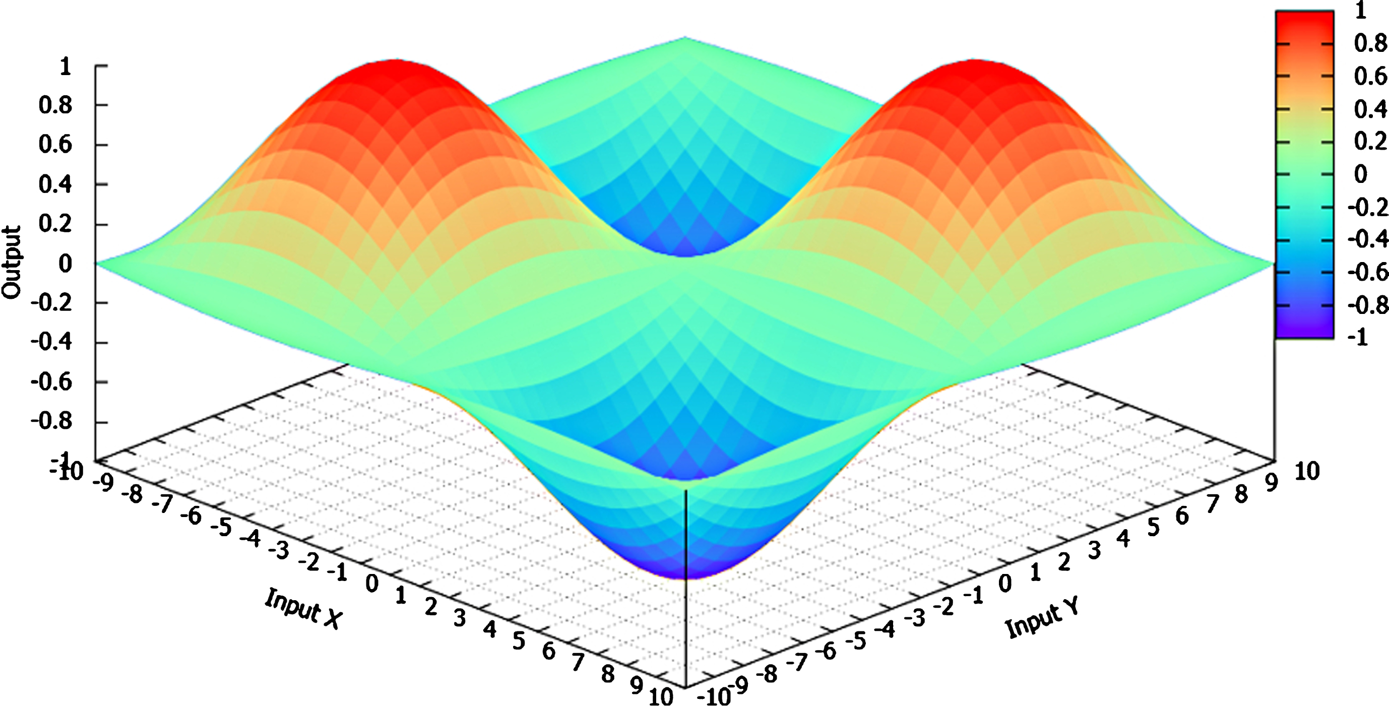
Problem space partition for the illustrative example.

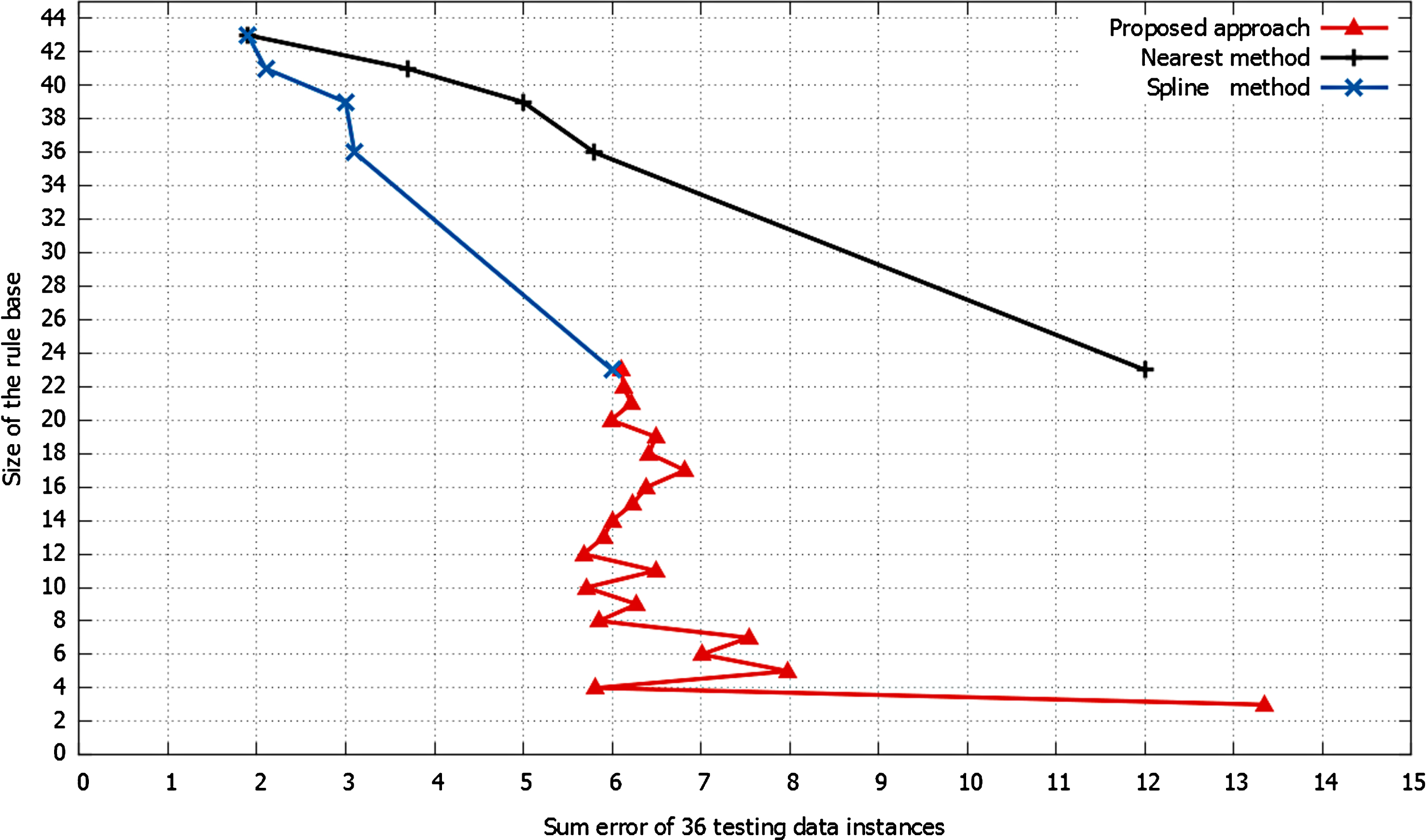
By employing the traditional similarity-based method in [17], if the number of rules is smaller than 23, the sum error of the testing instances is too high to be discussed. However, the proposed curvature-based method can still generate acceptable results, with the optimised sparse rule base using 23 or less rules, as listed in Table 1. This initialised rule base was optimised using GA. In this experiment, the population size was set to 100, the maximum number of generations was set to 1,000, and the probabilities of crossover and mutation were set to 0.8 and 0.01, respectively. The optimised rule base with 23 rules is summarised in Table 2.

To enable a comparative study, the summed errors from 36 random testing data points produced by different approaches based on various sizes of rule bases are illustrated in Fig.2. The black line represents the results generated by the nearest neighbour interpolation approach and the blue line represents the results produced by the piecewise polynomial cubic spline interpolation approach as reported in [17], whilst the red line represents the results generated by the proposed curvature-based sparse rule base generation approach.

Fig. 2

Sum error led by rule bases with different sizes.

Table 3

Curvature values of the decomposed cubes from the first instance

Cube Index	1	2	3	4	5	6	7	8	9	10	11
Curvature value	0.0494	0.0149	0.1472	0.0069	0.1189	0.0204	0.0496	0.0568	0.2812	0.2004	0.0558
Cube Index	12	13	14	15	16	17	18	19	20	21
Curvature value	0.0145	0.0305	0.0247	0.0732	0.0734	0.1314	0.0046	0.049	0.0264	0.0211

Table 4

The indexes of selected important instances

input 1	input 2	input 3	input 4	input 5	input 6	input 7	output	index
63	59	60	65	69	81	84	1	384
59	57	59	64	73	79	84	1	261
60	53	60	62	73	81	82	1	162
63	59	57	65	69	80	86	1	361
60	59	61	62	68	81	85	1	300
60	56	56	63	65	80	83	1	334
63	57	63	64	67	81	83	1	377
48	58	58	44	71	77	79	2	644
43	56	59	37	64	74	77	2	885
44	57	53	46	67	78	79	2	678
41	55	53	37	64	79	76	2	827
50	55	58	43	73	75	80	2	645
42	54	56	39	63	76	78	2	904
38	55	54	42	63	78	71	2	547
45	56	55	46	68	79	78	3	446
48	54	54	49	67	77	89	3	1187
48	57	49	53	62	79	87	3	1203
45	54	54	48	63	78	82	3	1028
51	57	54	55	62	87	81	3	1462
51	52	49	50	63	79	79	3	1090
51	52	52	56	68	79	87	3	1175
58	57	55	66	51	88	87	4	1734
56	53	51	59	50	84	84	4	1964
57	56	49	58	50	87	85	4	1810
64	54	52	58	52	89	88	4	1694
59	51	57	59	52	87	86	4	1545
58	51	56	58	50	88	88	4	1542
66	56	56	66	49	89	87	4	1635

Table 5

Experimentation results for comparison in Experiment 2 (two to seven features used by the proposed approach and seven features used by other compared approaches)

Previous Methods	PSO-NN	GSA-NN	PSOGSA-NN	FPSOGSA-NN	SVM	NAIVE BAYES
Accuracy (%)	64.66	77.53	83.28	95.16	92.68	90.47
Proposed Approach	7 features	6 features	5 features	4 features	3 features	2 features
Accuracy (%)	99.2	99.15	98.8	98.6	98.15	96.75

From Fig.2 ErrorsWithDifferentRules, it is clear that rule bases with fewer rules generally lead to larger summed error and poorer system performance, whilst rule bases with more rules generally result in smaller summed error and better performance. However, it should be noted that this is not always the case. For instance, the sum error produced by the rule base with 12 rules is smaller than that produced by the rule base with 17 rules. In fact, as shown in the figure, the rule bases with 12, 10, 8, and 4 rules in this experiment have demonstrated better performance. This is partly because these selected rules more efficiently represent the intrinsic characteristics of the data.

4.2. Experiment 2: Indoor environment localisation

Detecting users in an indoor environment based on the strength of Wi-Fi signals has a wide application domain. Deployable models have been developed in monitoring and tracking users based on the Wi-Fi signal strength of their personal devices. The applications of such models include locating users in smart-home systems, locating criminals in bounded regions, and obtaining the number of users on an access point. An indoor environment localisation dataset was employed in this experiment to validate and evaluate the proposed approach [44]. The dataset was collected in an indoor space by observing the signal strengths of seven Wi-Fi signals visible on a smart-phone. The dataset includes 2,000 instances, each with seven inputs and one output. Each input attribute is a Wi-Fi signal strength observed on the smart-phone, whilst the output decision class is one of the four locations.

In comparison to the synthetic dataset (where the required data can be obtained from anywhere in the space, thus resulting in a very dense dataset), the collected small dataset is irregular and sparse. In this case, due to the sparseness of the dataset, each data instance in the dataset is regarded as a high-dimensional hypercube and represented as a fuzzy rule if it is selected. In order to distinguish the data instances and to select the important instances, all high-dimensional hypercubes are broken down into $C_{7}^{2} = \frac{7!}{2! (7 - 2)!} = 21$ cubes. Following this, the curvature values of all these 21 cubes from each hypercube are calculated, using the mean curvature from the moving least-squares (MLS) surface method as introduced in CurvatureSection. The Gaussian scale parameter h in Equation 1 theta (which determines the width of the Gaussian kernel) was set to 0.35 in this experiment, and the number-of-neighbours parameter was set to 38. For simplicity, only the curvature values of the decomposed 21 cubes from the first instance are listed in Table 2, whilst all the other 1999 instances are omitted here due to the space limit. Following this, the accumulated virtual ‘curvature value’ of each hypercube was calculated, as the summation of all its corresponding decomposed 21 cubes.

Note that in the rule base generation process for classification problems, each output class should be covered in order to avoid misclassification. Therefore, when selecting instances or hypercubes, the candidates should be considered in tandem with the local higher curvature values, instead of the global higher ones. Otherwise, the candidates with higher curvature values may just belong to one or two output classes in this particular experiment. This dataset has 500 instances in each output class, with a total of 2,000 instances in all four output classes. Thus, in each class, m important instances are chosen to guarantee that all the output classes are covered. In other situations that involve an uneven distribution, the number of selected instances in each class can be adjusted accordingly. Based on their accumulated curvature values, for each output class, the most significant m instances or hypercubes within the output class were selected, simply by taking the first m hypercubes with the highest accumulated curvature values. Finally, the most important 4 * m hypercubes or instances were selected to jointly initialise the rule base.

Empirical study shows that, in this example, m = 7 produces the best performance. The result shows that although there are 2,000 instances, only 4 * 7 =28 important instances were needed to construct a sparse rule base, as summarised in Table 4. The initial rule base was optimised by applying the GA over the training dataset in fine-tuning the membership functions of the fuzzy sets which are involved in the 28 rules. The results produced by the proposed method using two to seven features and other approaches using seven features were compared, as shown in Table 4. The classification accuracy of the proposed method is 99.25%, which outperforms all the existing methods. Furthermore, using the FRI performance of the constructed intermediate rule bases, important features can also be identified; these appear in descending order as [5 , 2]. If all the seven input features are used, the accuracy is 99.25%. Instead, if only the most important two to six input features are used, the accuracy still remains good as 96.75%, 98.15%, 98.6%, 98.8%, and 99.15%, respectively. This clearly demonstrates the superior advantage of the proposed approach.

5. Conclusion

Conclusion This paper proposes a curvature-based sparse rule base generation method to support fuzzy rule interpolation. The approach first either partitions the problem domain into a number of hypercubes for problems with dense datasets, or represents each data point as a hypercube if only a small dataset is available. From this, the hypercubes are discriminated by effectively utilising the curvature values, and each important hypercube is represented as a fuzzy rule. The proposed method has led to very comparative results in the experiments, which demonstrates its potential for a wider range of real-world applications. One possible future direction of improvement is to mathematically extend the traditional curvature value calculation in a more effective way for higher dimensional problems, given that the current approach is combinational and thus requires high computational power. In addition, the approach needs to be further evaluated by large-scale real-world applications.

References

E.H.

Mamdani , Application of fuzzy logic to approximate reasoning using linguistic synthesis, Computers, IEEE Transactions on100(12) (1977), 1182–1191.

Takagi and

Sugeno , Fuzzy identification of systems and its applications to modeling and control, Systems, Man and Cybernetics, IEEE Transactions on15(1) (1985), 116–132.

Kóczy and

Hirota , Approximate reasoning by linear rule interpolation and general approximation, International Journal of Approximate Reasoning9(3) (1993), 197–225.

Huang and

Shen , Fuzzy interpolative reasoning via scale and move transformations, Fuzzy Systems, IEEE Transactions on14(2) (2006), 340–359.

Yang and

Shen , Adaptive fuzzy interpolation, Fuzzy Systems, IEEE Transactions on19(6) (2011), 1107–1126.

Yang and

Shen , Closedformfuzzy interpolation, Fuzzy Sets and Systems225 (2013), 1–22.

S.-M.

Chen and

Y.-C.

Chang , Weighted fuzzy interpola-tive reasoning for sparse fuzzy rule-based systems, Expert Systems with Applications38(8) (2011), 9564–9572.

G.I.

Molnárka ,

Kovács and

L.T.

Kóczy , Fuzzy rule interpolation based fuzzy signature structure in building condition evaluation, in: Fuzzy Systems (FUZZ-IEEE), 2014 IEEE International Conference on, IEEE, 2014, pp. 2214–2221.

Li ,

Yang ,

H.P.H.

Shum and

Tan , Intelligent home heating controller using fuzzy rule interpolation, in: The 15th UK Workshop on Computational Intelligence (UKCI'2015), 2015.

10.

Yang ,

Li ,

Fehringer ,

Barraclough ,

Sexton and

Cao , Intrusion detection system by fuzzy interpolation, in: 2017 IEEE International Conference on Fuzzy Systems (FUZZIEEE), 2017, pp. 1–6.

11.

Li ,

Yang ,

Fu ,

Chao and

Qu , Dynamic qos solution for enterprise networks using tsk fuzzy interpolation, in: 2017 IEEE International Conference on Fuzzy Systems (FUZZ-IEEE), 2017, pp. 1–6.

12.

Long ,

Tan ,

Organisciak ,

Yang and

Shao , Towards light-weight annotations: Fuzzy interpolative reasoning for zero-shot image classification, in: Proceedings of BMVC 2018, 29th British Machine Vision Conference on, 2018.

13.

Yang ,

Li ,

Chao ,

Hackney and

Flanagan , Job shop planning and scheduling for manufacturers with manual operations, Expert Systems. doi: 10.1111/exsy.12315

14.

Elisa ,

Li ,

Zuo and

Yang , Dendritic cell algorithm with fuzzy inference system for input signal generation, in: Lotfi,

Bouchachia,

Gegov,

Langensiepen,

McGinnity

(Eds.), Advances in Computational Intelligence Systems, Springer International Publishing, Cham, 2019, pp. 203–214.

15.

L.-X.

Wang and

J.M.

Mendel , Generating fuzzy rules by learning from examples, Systems, Man and Cybernetics, IEEE Transactions on22(6) (1992), 1414–1427.

16.

Z.C.

Johanyák and

Kovács , Sparse fuzzy system generation by rule base extension, in: Proceedings of 11th IEEE International Conference of Intelligent Engineering Systems (INES 2007), Budapest, Hungary, Citeseer, 2007, pp. 99–104.

17.

Bellaaj ,

Ketata and

Chtourou , A new method for fuzzy rule base reduction, Journal of Intelligent & Fuzzy Systems: Applications in Engineering and Technology25(3) (2013), 605–613.

18.

L.T.

Koczy and

Hirota , Size reduction by interpolation in fuzzy rule bases, Systems, Man, and Cybernetics, Part B: Cybernetics, IEEE Transactions on27(1) (1997), 14–25.

19.

C.-W.

Tao , A reduction approach for fuzzy rule bases of fuzzy controllers, Systems, Man, and Cybernetics, Part B: Cybernetics, IEEE Transactions on32(5) (2002), 668–675.

20.

Li ,

H.P.H.

Shum ,

Fu ,

Sexton and

Yang , Experiencebased rule base generation and adaptation for fuzzy interpolation, in: 2016 IEEE International Conference on Fuzzy Systems (FUZZ-IEEE), 2016, pp. 102–109.

21.

Tan ,

Li ,

Wonders ,

Chao ,

H.P.

Shum and

Yang , Towards sparse rule base generation for fuzzy rule interpolation, in: Fuzzy Systems (FUZZ-IEEE), 2016 IEEE International Conference on, IEEE, 2016, pp. 110–117.

22.

P.-C.

Chang ,

C.-H.

Liu and

R.K.

Lai , A fuzzy case-based reasoning model for sales forecasting in print circuit board industries, Expert Systems with Applications34(3) (2008), 2049–2058.

23.

Casillas ,

Cordón and

Herrera , Cor: A methodology to improve ad hoc data-driven linguistic rule learning methods by inducing cooperation among rules, IEEE Transactions on Systems, Man, and Cybernetics, Part B (Cybernetics)32(4) (2002), 526–537.

24.

Chebrolu ,

Abraham and

J.P.

Thomas , Feature deduction and ensemble design of intrusion detection systems, Computers & Security24(4) (2005), 295–307.

25.

L.A.

Zadeh , Quantitative fuzzy semantics, Information Sciences3(2) (1971), 159–176.

26.

Tikk ,

Joó ,

Kóczy ,

Várlaki ,

Moser and

T.D.

Gedeon Stability of interpolative fuzzy kh controllers, Fuzzy Sets and Systems125(1) (2002), 105–119.

27.

Bouchon-Meunier and

Valverde , A fuzzy approach to analogical reasoning, Soft Computing3(3) (1999), 141–147.

28.

Huang and

Shen , Fuzzy interpolation and extrapolation: A practical approach, Fuzzy Systems, IEEE Transactions on16(1) (2008), 13–28.

29.

Shen and

Yang , Generalisation of scale and move transformation-based fuzzy interpolation, Journal of Advanced Computational Intelligence and Intelligent Informatics15(3) (2011), 288–298.

30.

Yang and

Shen , Towards adaptive interpolative reasoning, in: 2009 IEEE International Conference on Fuzzy Systems, 2009, pp. 542–549.

31.

Yang ,

Chao and

Shen , Generalised adaptive fuzzy rule interpolation, IEEE Transactions on Fuzzy Systems25(4) (2017), 839–853.

32.

Naik ,

Diao and

Shen , Genetic algorithm-aided dynamic fuzzy rule interpolation, in: Fuzzy Systems (FUZZ-IEEE), 2014 IEEE International Conference on, 2014, pp. 2198–2205.

33.

Naik ,

Diao and

Shen , Dynamic fuzzy rule interpolation and its application to intrusion detection, IEEE Transactions on Fuzzy Systems26(4) (2018), 1878–1892.

34.

S.D.

Peckham , Profile, plan and streamline curvature: A simple derivation and applications, Proceedings ofGeomor-phometry (2011), 27–30.

35.

Yang and

Qian , Direct computing of surface curvatures for point-set surfaces, SPBG7 (2007), 29–36.

36.

Alexa ,

Behr ,

Cohen-Or ,

Fleishman ,

Levin and

C.T.

Silva , Computing and rendering point set surfaces, IEEE Transactions on Visualization and Computer Graphics9(1) (2003), 3–15.

37.

Goldman , Curvature formulas for implicit curves and surfaces, Computer Aided Geometric Design22(7) (2005), 632–658.

38.

Guillaume , Designing fuzzy inference systems from data: An interpretability-oriented review, IEEE Transactions on Fuzzy Systems9(3) (2001), 426–443.

39.

Z.-M.

Yeh , A systematic method for design of multivariable fuzzy logic control systems, IEEE Transactions on Fuzzy Systems7(6) (1999), 741–752.

40.

Ishibuchi and

Yamamoto , Rule weight specification in fuzzy rule-based classification systems, IEEE Transactions on Fuzzy Systems13(4) (2005), 428–435.

41.

Yang ,

Zuo ,

Chao and

Qu , Fuzzy interpolation systems and applications, in: Modern Fuzzy Control Systems and Its Applications, In Tech, 2017.

42.

Li ,

Yang ,

Qu and

Sexton , An extended takagi-sugeno-kang inference system (TSK+) with fuzzy interpolation and its rule base generation, Soft Computing22(10) (2018), 3155–3170.

43.

F.J.

Berlanga ,

Rivera ,

M.J.

del Jesús and

Herrera , Gp-coach: Genetic programming-based learning of compact and accurate fuzzy rule-based classification systems for high-dimensional problems, Information Sciences180(8) (2010), 1183–1200.

44.

J.G.

Rohra ,

Perumal ,

S.J.

Narayanan ,

Thakur and

R.B.

Bhatt , User localization in an indoor environment using fuzzy hybrid of particle swarm optimization & gravitational search algorithm with neural networks, in: Proceedings of Sixth International Conference on Soft Computing for Problem Solving, Springer, 2017, pp. 286–295.

Curvature-based sparse rule base generation for fuzzy rule interpolation

Abstract

Keywords

1. Introduction

2. Background

2.1. Rule base generation and reduction

2.3. Curvature

3.1. The basic case with two inputs

3.1.1. Problem domain partition

3.1.2. Curvature-based region selection

3.1.3. Rule base initialisation

3.2.1. Problem domain partition

3.2.2. Representing hypercube in cubes

3.2.4. Feature discrimination

3.2.5. Rule base initialisation

4. Experimentation

Table 1 The initialised rule base for Experiment 1

5. Conclusion

References

Table 1
The initialised rule base for Experiment 1