In this paper, we build a metric semi-linear space for lattice intuitionistic fuzzy numbers (LIFNs). We give new concepts of some operations, for example, a geometric binary addition operation, a nonnegative multiplication operation, geometric differences, and propose a new formula to calculate the derivative and integral of geometric lattice intuitionistic fuzzy functions in , we introduce and establish the positive solutions of the initial value problem for geometric lattice intuitionistic fuzzy differential equation (IVP for GLIFDE), and additionally show several practical applications in this semi-linear space with the medical intuitionistic fuzzy models.
In 1983, Atanassov introduced the concept of ”Intuitionistic fuzzy sets - IFSs” [2, 3]. It is a generalization of the fuzzy sets that it could be an important idea when describing a problem with a variable language (fuzzy) and was pretty useful in situations when describing a problem. Because of the flexibility of Intuitionistic fuzzy sets in handling uncertainty, they are a tool for a more human consistent reasoning under the undefined event perfect and vague. [12] used the same terminology "intuitionistic fuzzy set" as Atanassov but different in meaning to build the concept of intuitionistic fuzzy logic and IFSs. In the present time, the IFS theory has been applied to many different fields, for example, in [6] the author discussed intuitionistic fuzzy medical diagnosis consisting of three major steps: symptom identification, formulation of medical knowledge. In [11] the author had discussed an application of intuitionistic fuzzy multiset in medical diagnosis, in [4] the author proposed method of many measurement tools and multi-criteria decisionmaking.
Approach and objective
The main objective of this study is the intuitionistic fuzzy numbers (IFNs) which is related to the intuitionistic fuzzy sets (IFSs) [2, 3]. In the present approach, we will study them through L-fuzzy sets, which means us describe them as special cases of Goguen’s L-fuzzy sets [8] with elements taking values in a complete lattice [5], where
As we all know, the most real-world problems are studied through differential equations, since the structure of solutions of differential equations can explain many natural phenomena. One specific example is the fuzzy sets were introduced in 1965. However, more than 20 years later, people began to pay attention to its analytic structure, By launched the concept of the addition between two fuzzy sets and the scalar multiplication between a fuzzy set and a non-negative real number, these two operations along with Zadeh’s extended principle have been the basis for the development of semi-linear metric spaces of fuzzy sets, which has led to studies of fuzzy differential equations thrive. In recent years, there have been many studies revolving around the concept of "fuzzy differential equations". As for the intuitionistic fuzzy sets (IFSs), which K.A. Atanassov introduced in his researched since 1983. But until 1999, he began to present the operators on IFSs, so far there have been extensive research articles on these operators. Based on this ideas, Xu and Yager [10] defined the intuitionistic fuzzy numbers which are considered as the basic elements of the intuitionistic fuzzy sets. Most recently, In [1] the authors gave the definition of derivative operations for IFNs and their limited character analysis.
Consequently, from the above viewpoints, we built the basic foundations for IFNs in this paper. Specifically, we built the space for lattice intuitionistic fuzzy numbers (LIFNs) which are the IFNs when this IFNs located in . In addition, a problem that we need a mathematical analysis model to describe how time-varying intuitionistic fuzzy processes and to consider the structure of this model. Therefore, we introduce the concept of geometric lattice intuitionistic fuzzy functions, classify them and examine the derivatives and integrals of them. From the continuous, differentiability and integrable properties of the geometric lattice intuitionistic fuzzy functions, we build the initial value problem of geometric lattice intuitionistic fuzzy differential equation (IVP for GLIFDE). Moreover, to demonstrate the applicability of the results of this paper, we use the tool which is geometric lattice intuitionistic fuzzy differential equation on the space, to produce models for a disease state in a population at a certain time. Whereby, when a disease penetrates into a certain population, there will be two processes occur in this population. The first process is the increase in the number of infected members in the population, the second process is the decrease in the number of non-infected members in the population. To simulate a continuous dynamic system of this two processes in space, we assume that x1 (t) is process increasing and x2 (t) is process decreasing over time and .
Outline
This paper includes: In section 2, we collect the fundamental notions to use in the next section. In section 3, we proceed to construct two operations: addition operation () and scalar multiplication operation (), such that is a semi-linear space. Then we analyze the order in this semi-linear space to form the concept of geometric differences and provide a definition of the differentiable properties of geometric lattice intuitionistic fuzzy functions on . We introduce about the initial value problem of geometric lattice intuitionistic fuzzy differential equation (IVP for GLIFDE) and the medical intuitionistic fuzzy model that describes the developmental process of a disease in a population over time.
Preliminaries and notation
We recall some notations and concepts presented in detail in series of researches about fuzzy sets and its extended (see [2, 14]).
Definition 2.1. ([14]) Let U be a universe of discourse, then a fuzzy set
that it is characterized by membership function:
that means membership function μA (u) is continuous on [0, 1].
In [2, 3], the author introduced the concept of intuitionistic fuzzy sets (IFSs), it is characterized by a membership function and a non-membership function, which is a generalization of fuzzy sets (FSs).
Definition 2.2. [2, 3] Let U be a universe of discourse, then an intuitionistic fuzzy set A ={ (u, μA (u), νA (u)) |u ∈ U } that is characterized by membership function:
and by non-membership function:
that means membership function μA (u), and non-membership function are continuous on [0, 1] and satisfy 0 ≤ μA (u) + νA (u) ≤1 .
Based on this ideas, Xu and Yager [10] defined the intuitionistic fuzzy numbers which are a pair x = (μ, ν) ∈ [0, 1] × [0, 1] such that 0 ≤ μ + ν ≤ 1 . Next, we will reiterate the definition of semi-linear spaces, it will be useful for the next section of this study. Because our main purpose is to build a semi-linear space for the IFNs. Of course! If we can build a linear space for intuitionistic fuzzy numbers (IFNs) then it will be very perfect. However, even Zadeh’s fuzzy sets cannot establish a linear space that can only create a semi-linear space to them. The fuzzy sets (FS) was introduced in 1965. But more than 20 years later, people began interested in its analytic structure, by constructing the concept of semi-linear metric space of fuzzy sets, this has led to the study of fuzzy differential equations. In recent years, there have been many studies revolving around the concept of "fuzzy differential equations - FDEs". As for the Atanassov’s Intuitionistic fuzzy sets, They are not built a specific space. As such, studying them through analytical tools, namely differential equations, will be very difficultto develop.
Definition 2.3. [7, 13] A semi-linear space is a set S end owed with two operations, that means addition operation and scalar multiplication operation by nonnegative reals, which satisfy the following properties for every x, y ∈ S and λ, γ ∈ R+:
(S, +) is a commutative cancellative semi-group with 0,
λ (x+ y) = λx + λy;
(λ+ γ) x = λx + γx;
(λ . γ) x = λ (γx);
1x = x and 0x = 0 .
Example 2.1. From the definition 2.3, we have some examples of semilinear space (can see [2, 3]): any linear vector space is a semi-linear space, any linear topological vector space is a topological semi-linear space, any normed vector linear space is a metric semi-linear space. The most specific we can see the space of Zadeh’s fuzzy sets is a semi-linear space.
The property (i) in definition 2.3 implies that addition operation must satisfy the following three properties: x + y = y + x, (x + y) + z = x + (y + z) and x + 0 = x. If this addition operation has an extra property (where is called the reverse element of x) then the semi-linear space becomes the linear space. When there is a linear space (or semi-linear space) of an any set, we are easy to construct an analytic structure on it. In the next section, we will introduce two concepts of addition operation and scalar multiplication operation such that they can satisfy the properties in definition2.3.
Main Result
The metric semi-linear space of lattice intuitionistic fuzzy numbers
By Atanassov’s concept every intuitionistic fuzzy set (IFS) (see [2, 3]):
if we put x = (x1, x2) = (μA (u), νA (u)) then we have a rectangle
Definition 3.1. We denote
and classifying ≼G order in L* for ∀x, y ∈ L*:
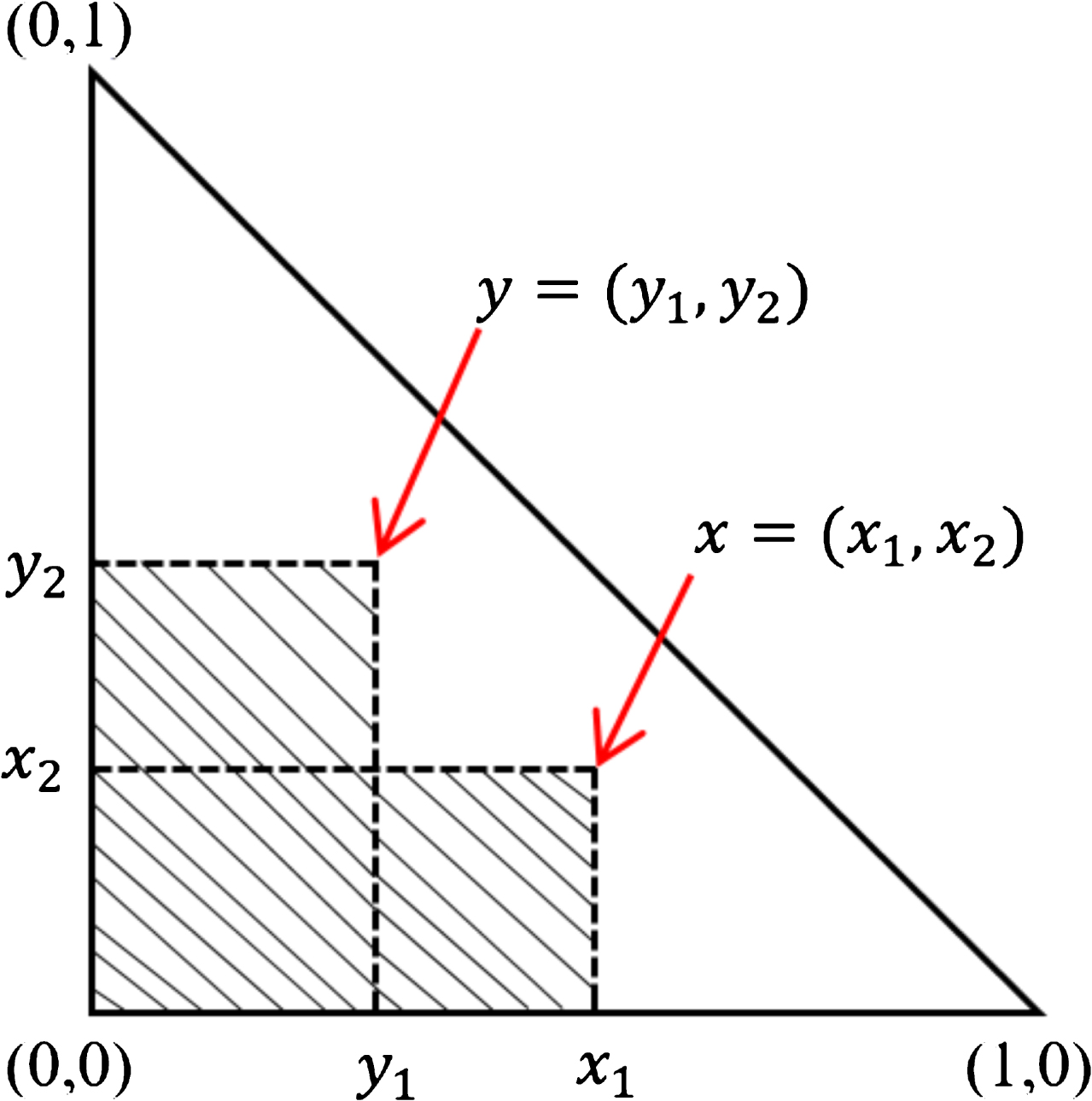
We say that is a complete lattice and every is called a lattice intuitionistic fuzzy number (LIFN). A simple description for the Definition 3.1 is provided in Fig. 1.
A geometrical interpretation of LIFNs y ≼ Gx in
Remark 3.1. In , each lattice intuitionistic fuzzy number corresponds to a fuzzy rectangle
Definition 3.2. We denote that:
is called the zero element of
if then is called the reverse element of
Remark 3.2. As we all know, before the concept of the intuitionistic fuzzy number appears, in mathematics, there existed a concept which is "interval". Based on the definition of the closed interval, if , we always have a ≤ b and there is no reverse case. For example, we have [0, 2] while [2, 0] does not satisfy the definition of an interval. Similarly, we have the concept of an open-ended interval. In the general case, if (or using symbol] a, b [to represent an open-ended interval), we always have a < b and there is no reverse case. For example, we have (0, 2) while (2, 0) does not satisfy the definition of an interval. However, with a intuitionistic fuzzy number x = (x1, x2), then x1 may be larger than x2 or vice versa. For example, we have the IFN x = (x1, x2) = (0.2, 0.7) and the IFN y = (x2, x1) = (0.7, 0.2). Nevertheless, in some special cases, the IFNs are mathematically equivalent to the intervals, for example, we have a closed interval [0, 0.8] (or an open-ended interval (0, 0.8)) and we also have a IFN (0, 0.8) . Therefore, we need to distinguish that the difference of arithmetic operations of these two objects. Specifically, we have some arithmetic operations for intervals by endpoint formulas the following (can see [9]): [a, b] + [c, d] = [a + b, c + d] (addition), [a, b] - [c, d] = [a - d, b - c] (subtraction), and for all we have k . [a, b] = [ka, kb] if k ≥ 0 or k . [a, b] = [kb, ka] if k < 0 (scalar multiplication). However, These three operators are not suitable for IFNs, for example, giving two IFNs x = (0.3, 0.6) and y = (0.8, 0.1) then x + y = (1.1, 0.7) ∉ L*, x - y = (-0.5, 0.5) ∉ L*, and k . x = (k . 0.6, k . 0.3) ∉ L* if k < 0 . Therefore, for the IFNs, we need to rebuild the appropriate arithmetic operations on L* .
Remark 3.3. We can give some kinds of the binary addition operators in , for example:
the coordinate addition operation of two elements of , that denote by z = x+ y = (x1 + y1, x2 + y2);
the logical addition operation of two elements of , that denote by z = x+ y = (x1 + y1 - x1y1, x2 . y2);
the average addition operation of two elements of , that denote by
In family of the intuitionistic fuzzy numbers all above kinds of the binary addition operators will only satisfy the commutative property, but without satisfying the distributed property. To have a binary addition operation with both properties, we will extend the average addition operation ⊕ of two elements (without losing the properties of the double addition) by the other concept of close addition operation ⊕G in as follows:
Definition 3.3. Let m elements we say that there exists an geometric addition operation of this m elements as follows: iff
with p is number of component x(j) = (0, 0) = θ, j = 1, 2, …, m and satisfy
where n ≤ m .
Definition 3.4. We say that there exists an geometric binary addition operation of two elements of as follows:
if both x and y are different from zero elements in (that means x ≠ θ = (0, 0) and y ≠ θ = (0, 0)), that means m = 2, p = 0.
The properties of this geometric binary addition operation in Definition 3.4 will be in the following Theorem 3.2. To easily visualize the geometric binary addition operation in Definition 3.4, we will provide some simple examples.
Example 3.1. Now, we consider the geometric binary addition operation with two elements in , for and , from the Definition 3.4, then we have , It is clear that z belongs to because z satisfies 0 ≤ 0.4 + 0.45 ≤ 1. The illustration for the case of the geometric binary addition operation with two elements in is represented in Fig. 2. But assuming that and then p = 1 and m = 2, so we have .
The next, we consider the geometric binary addition operation with three elements in , for three elements x = (x1, x2) = (0.1, 0.9), y = (y1, y2) = (0.8, 0.2) and t = (t1, t2) = (0.2, 0.7) clearly all these three elements belong to . All three elements x, y, t are different from θ = (0, 0) implies that p = 0 and because the geometric binary addition operation has three elements, we have m = 3. Thus .
An important point in Definition 3.3 are two conditions i/ and ii/, we will explain in detail why these two conditions must have. Specifically, when we examine the properties in Definition 2.3, then the property (x ⊕ Gy) ⊕ Gz = x ⊕ G (y ⊕ Gz) is not satisfied, because (x ⊕ Gy) ⊕ Gz ≠ x ⊕ G (y ⊕ Gz). For example, let then (x ⊕ Gy) ⊕Gz = , = (0.4, 0.5) = and x ⊕G (y ⊕ Gz) = , = (0.425, 0.525) = . We see v ≠ w. Therefore, we add to the Definition 3.3 with two conditions i and ii, in order to property (x ⊕ Gy) ⊕ Gz = x ⊕ G (y ⊕ Gz) can be satisfied. From the example above, by using two conditions i/, ii/ in the Definition 3.3 with m = 3 and n = 2, we have .
Corollary 3.1.For three elements and x, y, z ≠ θ then the extended geometric addition operation in Definition 3.3 satisfies:
Geometric binary addition operation of the LIFNs
Proof. (x ⊕ Gy) ⊕ Gz = x ⊕ G (y ⊕ Gz) ? Particular, using the extended geometric addition operation by Definition 3.3 in the case m = 3, n = 2, p = 0 then we have:
Theorem 3.2.The geometric binary addition operation in Definition 3.4 with the extended geometric addition operation in Definition 3.3 of the lattice intuitionistic fuzzy numbers satisfies:
x⊕ Gy = y ⊕ Gx;
(x⊕ Gy) ⊕ Gz = x ⊕ G (y ⊕ Gz);
Proof. We prove this properties of geometric binary addition operation of the lattice intuitionistic fuzzy numbers by Definition 3.4: x ⊕ Gy = y ⊕ Gx ? Particular, because xi, yi ∈ [0, 1], i = 1, 2, m = 2, p = 0 then we have:
2/ (x ⊕ Gy) ⊕ Gz = x ⊕ G (y ⊕ Gz) ? Particular, because 0 ≤ x1 + x2 ≤ 1 and using the extended geometric addition operation of the lattice intuitionistic fuzzy numbers by Definition 3.3 and Corollary 3.1 the case m = 3, n = 2, p = 0 . Particular, because 0 ≤ x1 + x2 ≤ 1 and using the geometric binary addition operation of the lattice intuitionistic fuzzy numbers by Definition 3.4 in the case m = 2, p = 1 then we have:
□
Remark 3.4.By the Theorem 3.2 the new closed binary addition operation ⊕G in satisfies that is a binary addition of two elements of . This mathematical operation ⊕G in is a commutative and distributive extended binary addition operator.
Definition 3.5. Let we say that there exists a nonegative scalar multiplication operation if 0 ≤ λ . x1 + λ . x2 ≤ 1, and denote
Theorem 3.3.Assuming that the scalar multiplication operation in Definition 3.5 is exists then it’s satisfies:
λ⊙ (x ⊕ Gy) = λ ⊙ x ⊕ Gλ ⊙ y;
(λ+ β) ⊙ x = λ ⊙ x + β ⊙ x;
(λ . β)⊙ x = λ ⊙ (β ⊙ x);
where + is an coordinate addition operation and ⊕G is the new concept of geometric binary addition operation in .
Proof. We have to prove this properties of the scalar multiplication operation in Definition 3.5:
1/ λ ⊙ (x ⊕ Gy) = λ ⊙ x ⊕ Gλ ⊙ y ? Particular, because xi, yi ∈ [0, 1], i = 1, 2, m = 2, p = 0 then we have:
2/ (λ + β) ⊙ x = (λ ⊙ x) + (β ⊙ x) ? Particular, because then we have:
3/ (λ . β) ⊙ x = λ ⊙ (β ⊙ x) ? Particular, because x1, x2 ∈ [0, 1] and then we have:
4/ Particular, because xi ∈ [0, 1], i = 1, 2 then we have:
5/ Particular, because xi ∈ [0, 1], i = 1, 2 then we have:
Definition 3.6. The geometric distance between intuitionistic fuzzy numbers denote by
Theorem 3.4.The geometric binary addition operation in Definition 3.4, the scalar multiplication operation in Definition 3.5 of the lattice intuitionistic fuzzy number on and the geometric distance between two lattice intuitionistic fuzzy numbers in Definition 3.6 make that become to the metric semi-linear space of the lattice intuitionistic fuzzy numbers (LIFNs).
Proof. From Definition 2.3, using Theorems 3.2 – 3.3, we have is a semi-linear space and Definition 3.6 we get the metric semi-linear space of the lattice intuitionistic fuzzy numbers.□
The geometric lattice intuitionistic fuzzy functions
Definition 3.7. Let , with and t, t + h ∈ [t0, T], ∀ h > 0 . We say that
the geometric lattice intuitionistic fuzzy function x (t) is strict monotone increasing by t iff x (t) ≼ G1x (t + h) in with x1 (t)≤ x1 (t + h), x2 (t + h) ≤ x2 (t), ∀ t ∈ [t0, T];
there is exist a geometric difference under first type iff y (t) ≼ G1x (t) in and y1 (t) ≤ x1 (t), x2 (t) ≤ y2 (t), ∀ t ∈ [t0, T] where (z1 (t), z2 (t)) = (x1 (t) - y1 (t), y2 (t) - x2 (t)) = (x1 (t) - y1 (t), - (x2 (t) - y2 (t))) .
Definition 3.8. Let , with and t, t + h ∈ [t0, T], ∀ h > 0 . We say that
the geometric lattice intuitionistic fuzzy function x (t) is monotone decreasing by t iff x (t + h) ≼ G2x (t) in with x1 (t+ h) ≤ x1 (t), x2 (t) ≤ x2 (t + h), ∀ t ∈ [t0, T];
there is exist a geometric difference under second type iff y (t) ≼ G2x (t) in and x1 (t) ≤ y1 (t), y2 (t) ≤ x2 (t), ∀ t ∈ [t0, T] where (z1 (t), z2 (t)) = (y1 (t) - x1 (t), x2 (t) - y2 (t)) = (- (x1 (t) - y1 (t)), x2 (t) - y2 (t)) .
If exist or then we say that exists and is called geometric difference (with symbol
Theorem 3.5.Assume that , with geometric difference then there are exist the following properties:
If x (t) y (t), x (t) z (t) exist, then [x (t) y (t), x (t) z (t)] = [y (t), z (t)];
If , exist, then there exist and
The same result when replacing by
Proof. (a/) Suppose that , exist, from Definition 3.6, we have , and , so
(b/) Suppose that x (t) y (t), x (t) z (t), z (t) exist, this implies that x (t) y (t) ∈ , x (t) z (t) ∈ L* and z (t) y (t) ∈ . Thus [x (t) z (t)] ∈ and
□
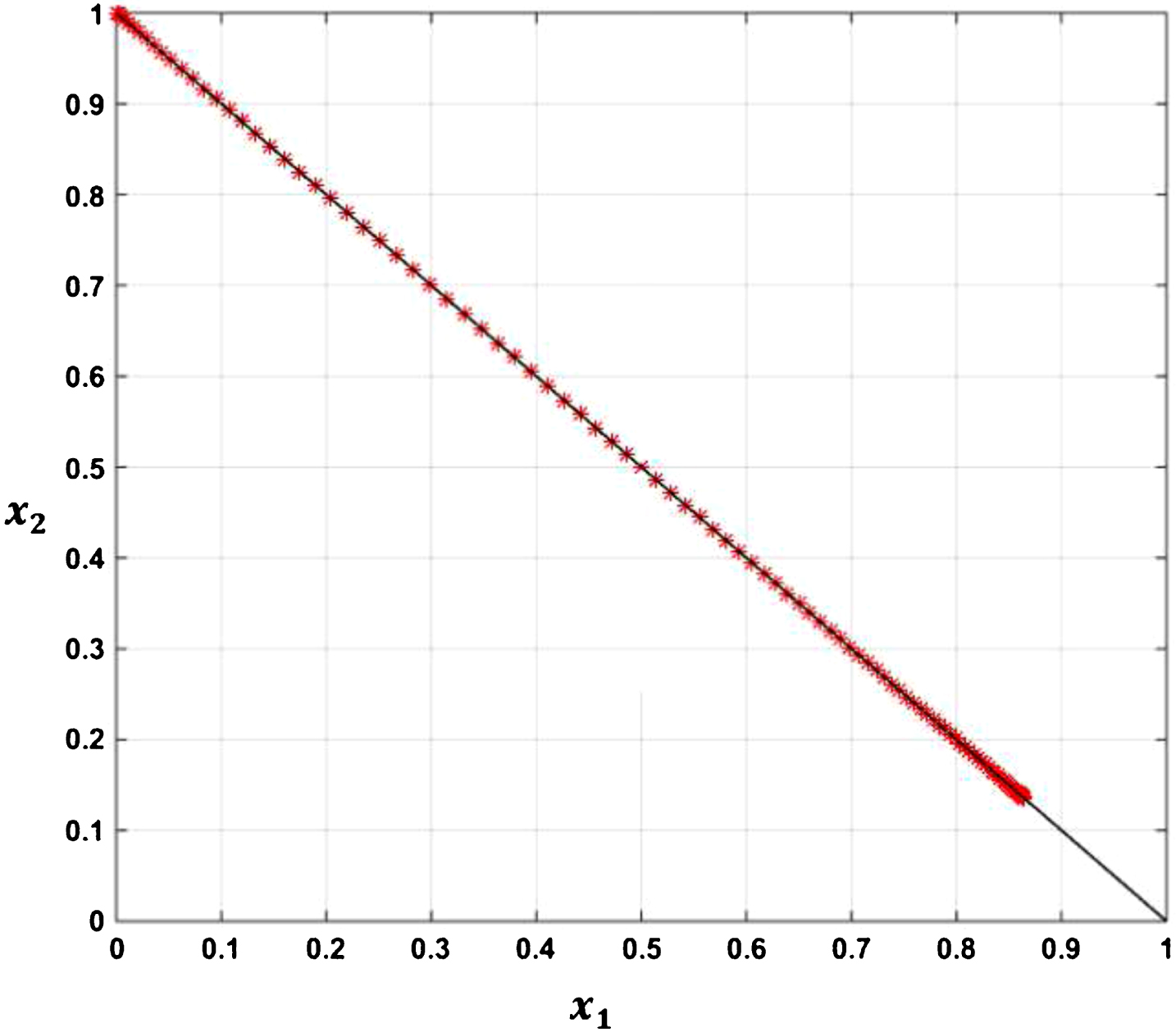
Illustration of the real functions x1 (t), x2 (t) belong to C (R, [0, 1]), with x1 (t) + x2 (t) =1 .
In order to have an intuitive view of the continuous intuitionistic fuzzy functions in , we recognize that each of the functions is represented by the form x (t) = (x1 (t), x2 (t)), where xi (t), i = 1, 2 are the continuous functions on the [0, 1] . So we have a relationship between the continuous real functions and the continuous geometric lattice intuitionistic fuzzy functions in the metric semi-linear geometric lattice space of LIFNs, we can assume the functions xi (t) with the graph shown in Fig. 3, at each tk, k = 1, 2 we have the point Mk = (x1 (tk), x2 (tk)). The Fig. 4 below shown geometrical interpretation of geometric lattice intuitionistic fuzzy functions in
Illustration of the geometric lattice intuitionistic fuzzy functions x (t) = (x1 (t), x2 (t)) belong to in the case x1 (t) + x2 (t) =1 .
Definition 3.9. Let . We say that a geometric lattice intuitionistic fuzzy function x (t) is geometric differentiable at t ∈ (t0, T), if there are exist the geometric differences and , such that
or if there exists geometric differences and , such that
where denote DGx (t) is geometric derivatives in
Theorem 3.6.The geometric derivative of the geometric lattice intuitionistic fuzzy function will have the following form:
if the geometric lattice intuitionistic fuzzy function x (t) is strict monotone increasing by t;
if the geometric lattice intuitionistic fuzzy function x (t) is monotone decreasing by t .
Proof. a/ Because the geometric lattice intuitionistic fuzzy function x (t) is strict monotone increasing by t then exists and implies that x (t) ≼ G1x (t + h) or x1 (t) ≤ x1 (t + h), x2 (t + h) ≤ x2 (t). By Definition 3.7, we have and
b/ Because the geometric lattice intuitionistic fuzzy function x (t) is monotone decreasing by t then exists and implies that x (t) ≼ G2x (t + h) or x1 (t + h) ≤ x1 (t), x2 (t) ≤ x2 (t + h) . By Definition 3.8, we have and
□
The initial value problem of geometric lattice intuitionistic fuzzy differential equation in
For every , we have the initial value problem for geometric lattice intuitionistic fuzzy differential equation (IVP for GLIFDE) under form:
where that means and DGx (t) is geometric derivative of x (t) . A special point of the problem (3.2) is that it can be rewritten into a system of real equations. Because so
with x1 (t), x2 (t), f1 (.), f2 (.), x1 (t0), x2 (t0) ∈ [0, 1] and
Assume that the geometric derivative of geometric lattice intuitionistic fuzzy function x (t) is DGx (t) exists then the problem (3.2) can be written as follows: In the case, when the geometric lattice intuitionistic fuzzy function x (t) is strict monotone increasing by t . Then the problem 3.2 be written as:
In the case, when the geometric lattice intuitionistic fuzzy function x (t) is monotone decreasing by t . Then the problem 3.2 be written as:
Example 3.7. Let consider the initial value problem of geometric lattice intuitionistic fuzzy differential equation (IVP for GLIFDE) under the form:
with x (t) is a strict monotone increasing function by t .
We find the solutions of (IVP for GLIFDE) (3.3). Because x (t) is a strict monotone increasing function, thus (IVP for GLIFDE) (3.3) be written as follows:
Solving (3.4), we have one of the solutions of (IVP for GLIFDE) (3.3) that is
Illustration of the real functions x1 (t), x2 (t) belong to C ([0, 4], [0, 1]) .
Solution of (IVP for GLIFDE) (3.3) in for Example 3.7.
Example 3.8. Let consider the initial value problem of geometric lattice intuitionistic fuzzy differential equation (IVP for GLIFDE) under the form:
with x (t) is a monotone decreasing function by t .
We find the solutions of (IVP for GLIFDE) (3.5). Because x (t) is a monotone decreasing function, thus (IVP for GLIFDE) (3.5) be written as follows:
Solving (3.6), we have one of the solutions of (IVP for GLIFDE) (3.5) that is
and it’s graph illustrates in Figs. 7 and 8.
Illustration of the real functions x1 (t), x2 (t) belong to
Solution of (IVP for GLIFDE) (3.5) in for Example 3.8.
The medical applications
In this paper, we use the tool that is geometric lattice intuitionistic fuzzy differential equation on space, to produce models for a disease state in a population at a certain time. According to our observation, when a disease penetrates into a certain population, there will be two processes occur in this population. The first process is the increase in the number of infected members in the population, the second process is the decrease in the number of non-infected members in the population. To simulate a continuous dynamic system of this two processes in space, we assume that x1 (t) is process increasing and x2 (t) is process decreasing over time and x (t) = (x1 (t), x2 (t)) ∈ (L*, ≼ G). We introduce a model describing the developmental process of a disease in a population over time in the following form:
where x (t) = (x1 (t), x2 (t)), f (t, x (t)) = (f1 (.), f2 (.)) ∈ , “⊙” is the symbol of the scalar multiplication operation in the definition 3.5, DGx (t) is geometric derivative of x (t) and u (t) ∈ [0, 1] is control real function (pills and other preventions). In addition, x1 (t) =1 - x2 (t) and at the time of the original x1 (t0) =0, x2 (t0) =1, this implies that at the initial time the number of infected members is 0% and the number of non-infected members is 100% in the population. In fact, when a disease invades a population, it will encounter some obstacles, for example, vaccines, pills and other preventions, thus we add to the u (t) control real function to the above model, to express the effect of drugs on this disease. Because x1 (t) is increases process and x2 (t) is process decreasing over time, thus is strict monotone increasing function in and (3.7) will be the dynamic system of the form:
Solving of system (3.8), we have solutions x1 (t), x2 (t) are real positive processes in [0, 1] with condition 0 ≤ x1 (t) + x2 (t) ≤1, thus is positive solutions of system (3.8). Specifically, we have
and .
Example 3.9. Let consider one model describing the developmental process of a disease in a population over time with x1 (t) is increases and x2 (t) is decreases then the model that describes the developmental process of a disease in a population for relationship between x1 (t), x2 (t) ∈ [0, 1] and the control real functions u (t) (pills and other preventions) will be:
Because x1 (t) is process increasing and x2 (t) is process decreasing over time, thus is strict monotone increasing function and (3.9) be written as under type:
Assume that u (t) = sin(t).
Solving (3.10), we have the general solutions:
with and x (0) = (0, 1) = (C1, C2), then finally we have:
Hence, is a solution of the IVP for GLIFDE (3.9). This solution is shown in Figs. 9 and 10. The numerical simulation for solutions of Example 3.7, 3.8, and 3.9 are provided in Table 1.
Illustration of the real functions x1 (t), x2 (t) belong to C ([0, π], [0, 1]) .
Solution of (IVP for GLIFDEs) (3.9) in for Example 3.9.
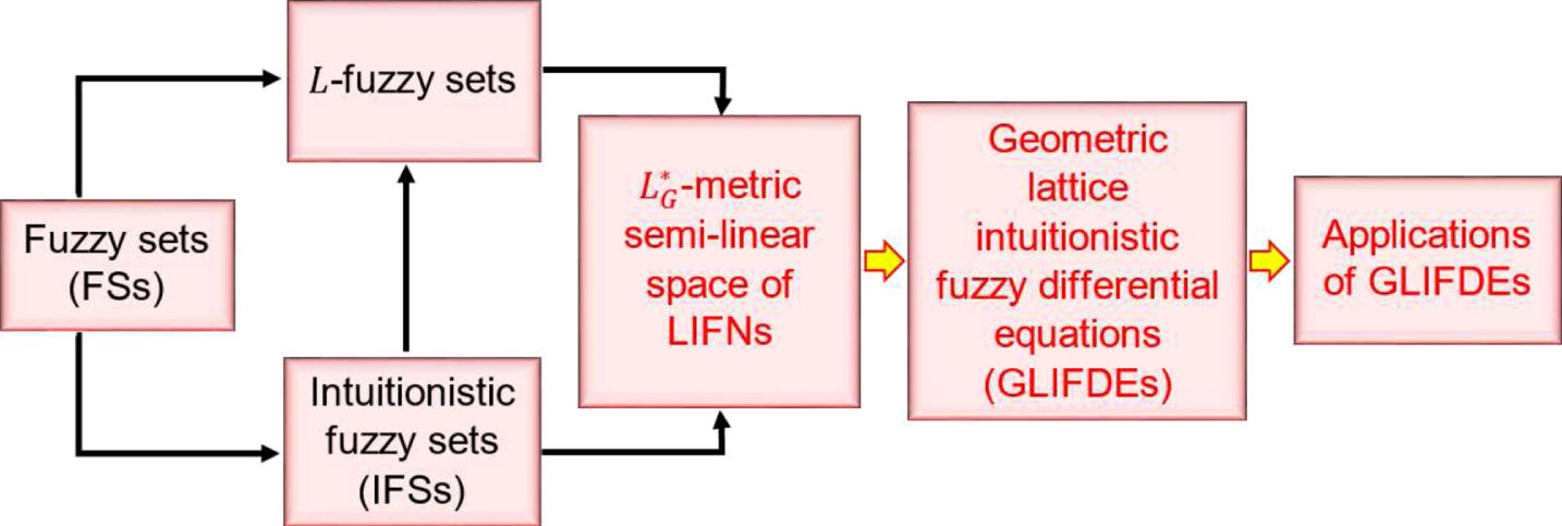
We have the diagram illustrates the relationship between some kinds of fuzzy sets and
is the metric semi-linear space of lattice intuitionistic fuzzy numbers (Fig. 11).
The diagram illustrates the relationship between some kinds of fuzzy sets, the metric semi-linear space of the lattice intuitionistic fuzzy numbers – LIFNs and GLIFDEs. Last three boxes are the new.
Table1
Numerical simulation for solutions of Example 3.7, 3.8, and 3.9.
Example 3.7
Example 3.8
Example 3.9
t
x (t) = (x1 (t), x2 (t))
t
x (t) = (x1 (t), x2 (t))
t
x (t) = (x1 (t), x2 (t))
0.0000
(0.0000000, 1.0000000)
0.0000
(1.0000000, 0.0000000)
0.0000
(0.0000000, 1.0000000)
0.4000
(0.3296799, 0.6703200)
0.1571
(0.9876883, 6.4516e-04)
0.3142
(0.0477651, 0.9522349)
0.8000
(0.5506710, 0.4493289)
0.3142
(0.9510565, 0.0051422)
0.6283
(0.1738533, 0.8261466)
1.2000
(0.6988057, 0.3011942)
0.4712
(0.8910065, 0.0172483)
0.9425
(0.3378179, 0.6621820)
1.6000
(0.7981034, 0.2018965)
0.6283
(0.8090169, 0.0405332)
1.2566
(0.4989167, 0.5010832)
2.0000
(0.8646647, 0.1353352)
0.7854
(0.7071067, 0.0782913)
1.5708
(0.6321205, 0.3678794)
2.4000
(0.9092820, 0.0907179)
0.9425
(0.5877852, 0.1334608)
1.8850
(0.7299145, 0.2700854)
2.8000
(0.9391899, 0.0608100)
1.0996
(0.4539904, 0.2085509)
2.1991
(0.7956222, 0.2043777)
3.2000
(0.9592377, 0.0407622)
1.2566
(0.3090169, 0.3055805)
2.5133
(0.8361849, 0.1638150)
3.6000
(0.9726762, 0.0273237)
1.4137
(0.1564344, 0.4260283)
2.8274
(0.8578761, 0.1421238)
4.0000
(0.9816843, 0.0183156)
1.5708
(0.0000000, 0.5707963)
3.1416
(0.8646647, 0.1353352)
Conclusions
The intuitionistic fuzzy theory has many implications for the perception of uncertain natural and social processes, that are applied to medical models, sales analytic models, and so on. We have built the space structure for a complete lattice with the name ”the metric semi-linear space” of lattice intuitionistic fuzzy numbers (LIFNs). In addition, we have new concepts about the geometric lattice intuitionistic fuzzy functions, geometric differentiability and the IVP for GLIFDE. We have the structure and positive solutions of this IVP for GLIFDE. For the applications, we have considered the model that describes the developmental process of a disease in a population that modifies the relationship between the proportion of x1 (t) is process increasing and x2 (t) is process decreasing over time.
Footnotes
Acknowledgments
The authors are deeply grateful to the reviewers and the editor for their careful reading and constructive comments.
References
1.
Z.Ai, Z.Xu and Q.Lei, Limit properties and derivative operations in the metric space of intuitionistic fuzzy numbers, Fuzzy Optim Decis Making. 10.1007/s10700-016-9239-7
2.
K.T.Atanassov, Intuitionistic fuzzy sets, VII ITKR's Session, Sofia, 1983.
3.
K.T.Atanassov, Intuitionistic fuzzy sets, Fuzzy Sets and Systems20 (1986), 87–96.
4.
K.T.Atanassov, G.Pasi and R.Yager, Intuitionistic fuzzy interpretations of multi-criteria multi-person and multi-measurement tool decision making, Int J of Systems Science36 (2005), 859–868.
5.
C.Cornelis, G.Deschrijver and E.E.Kerre, Implication in intuitionistic fuzzy and interval-valued fuzzy set theory: Construction, classiiňAcation, application, Int J of Approximate Reasoning35 (2004), 55–95.
6.
S.K.De, R.Biswas and A.R.Roy, An application of intu-itionistic fuzzy sets in medical diagnostic, Fuzzy Sets and Systems117 (2001), 209–213.
7.
G.N.Galanis, Differentiability on semi-linear spaces, Nonlinear Analysis71 (2009), 4732–4738.
8.
J.A.Goguen, L-fuzzy sets, J of Math Anal and Appli18 (1967), 145–174.
9.
R.E.Moore, R.B.Kearfott and M.J.Cloud, Introduction to interval analysis, So for Ind and App Math Philadelphia, SIAM (2009).
10.
Z.S.Xu and R.R.Yager, Some geometric aggregation operators based on intuitionistic fuzzy sets, Int J Gen Syst35 (2006), 417–433.
11.
T.K.Shinoj and J.J.Sunil, Intuitionistic fuzzy multisets and its application in medical diagnosis, Int J ofMathematical, Computational, Physical, Electrical and Computer Engineering6 (2012), 34–38.
12.
G.Takeuti and S.Titani, Intuitionistic fuzzy logic and intuitionistic fuzzy set theory, J Symbolic Logic49 (1984), 851–866.
13.
R.E.Worth, Boundaries of semilinear spaces and semialge-bras, Trans Amer Math Soc148 (1970), 99–119.