A rule activation method for extended belief rule base with VP-tree and MVP-tree

Abstract

The belief rules are stored out of order in the extended belief rule base (EBRB), which will weaken its reasoning performance in that all rules are visited when calculating each rule’s activation weight. This paper focuses on reducing the number of rules which are visited in the calculation of each rule’s activation weight. A new rule activation method based on VP-tree and MVP-tree is proposed to build index structure to store rules. The proposed rule activation method is based on rule similarity query, where only partial rules will be retrieved and visited while calculating each rule’s activation weight. Note that, the performance of EBRB systems based on tree index is affected greatly by the value of query threshold. However, sometimes it is difficult to determine the value of query threshold, so this paper also proposes an approach based on the k-means clustering algorithm to choose the appropriate query threshold. Some case studies show how the use of the proposed optimization method enhances the reasoning performance of EBRB systems. The proposed method has been validated to be advantageous to visit partial suitable rules instead of all rules. Beside the work performed in the EBRB, the proposed method alone can also be used in different application areas.

Keywords

Extended belief rule base rule activation method VP-Tree MVP-Tree

1 Introduction

Expert system (ES), one of the most active branches of Artificial Intelligence (AI), is widely used in commercial and industrial settings, including medicine, finance, manufacturing and sales. The belief rule base (BRB) system, a more generalized expert system, is capable of addressing various types of information which is qualitative or quantitative, linguistic or numerical, complete or incomplete. The belief rule base inference methodology using the evidential reasoning approach (RIMER) proposed by Yang [10], is developed on the basis of Dempster-Shafer theory of evidence [2, 3], decision theory [4], fuzzy set theory [1] and traditional IF-THEN rule-based method [7]. This methodology provides a more flexible way to represent knowledge and is able to capture vagueness, impreciseness, incompleteness and nonlinear relationship between antecedent attributes and an associated consequent. The RIMER approach along with the BRB has been proved to be applied in different application areas, such as, safety and risk analysis, health care, oil pipe leak detection and some other application in engineering systems [12–15 , 29].

In order to improve the reasoning performance of the BRB, there have been extensive studies in recent literature with respect to the parameter learning for the BRB. Yang [11] proposed the first generic BRB parameter learning framework with an optimization model. Then Chen [18] took referential values of antecedent attributes into account and proposed a global optimization model. Since these approaches are offline, Zhou [17] proposed an online updating approach which still requires the attributes to be discretized first. Subsequently, some other parameter learning methods using the swarm intelligence algorithm were proposed [20, 24]. However, for these models in essence are based on iterative search algorithms, it is time-consuming to train and re-train the parameters of the BRB. Later Liu [19] extended the BRB by embedding the belief degrees in the entire antecedent attributes of each rule, which is called the extended belief rule base (EBRB). More importantly, a novel belief rule generation mechanism which can generate such extend belief rule from numerical data directly was proposed. Owing to the novel features of the EBRB, it can handle the ambiguity contained not only in the consequent but also in the antecedent attribute and requires no time-consuming and iterative training procedures, but keeps the relatively good performance. The EBRB system has been widely used in solving the oil pipeline leak detection and software defect detection problems [19, 25].

Nevertheless, since the belief rules of an ERBB are stored out of order, it is inevitable to visit all rules when calculating the activation weight of each rule in the inference procedure. In addition, it is likely that the noise or unreliable data is commonly included in the EBRB. When there are too many belief rules in an ERBB, its reasoning performance will be lowered due to higher time cost and the quality of dataset. Therefore, it is highly essential to reduce the number of rules involved in the rule activation procedure by traversing and activating several important rules. Some studies in recent literature have attempted to deal with these problems in EBRB systems. Yu [21] proposed an activation method integrating only 20% activated rules in the inference process based on 80/20 principle. However, this method still needs to visit all rules when calculating the activation weight of each rule. The dynamic rule activation (DRA) method proposed by Calzada [26] selects a suitable set of activated rules in a dynamic way to address the incompleteness and inconsistency in EBRB systems. In this case, the increase of time should be taken into account since it involves time-consuming iterative procedures. Su [28] introduced a structure optimization framework with the Burkhard-Keller tree (BK-tree) [30] and a new method to calculate individual matching degree for EBRB systems. It is an excellent method to avoid visiting all rules when calculating each rule’s activation weight by retrieving nearest rules with the help of query thresholds. However, there was no mention about how to select appropriate query thresholds since it is difficult to determine the value of query threshold for some EBRB systems based on tree index structure. Because if the query threshold is too large, all rules will be retrieved, which means that it is superfluous to build BK-tree for EBRB. But if the query threshold is too small, then the issue that none of rules will be activated can happen.

To tackle the aforementioned issues in the EBRB system, this paper proposes a rule activation method by building index structure and clustering. Numerous approaches can help to meet this challenge, of which three approaches are applied in this paper: the vantage point tree (VP-tree), the multi-vantage point tree (MVP-tree) and the k-means algorithm. VP-tree [5, 6] and MVP-tree [8] are both solutions to the problem of finding data items similar to a given query item via building index structure. MVP-tree is an improvement on VP-tree with more vantage points. In recent years, VP-tree and MVP-tree have been widely used in the pattern recognition, text and image search [9, 22]. The k-means algorithm is one of the most popular and most commonly used clustering methods. In this paper, to address the issue that ERBB systems need to visit all rules while calculating each rule’s activation weight, a rule activation method based on VP-tree and MVP-tree is proposed to visit fewer but more representative belief rules. The EBRB systems based on VP-tree and MVP-tree can answer similarity-based queries efficiently by establishing index structure according to the similarity between rules. When calculating activation weight for each rule, only several rules will be retrieved and visited in terms of a query threshold, which can be specified in the beginning or determined by the k-means algorithm, so that the reasoning performance of EBRB systems can be boosted. The main advantage of the proposed method is its flexibility because it can be combined with any EBRB systems or other systems with belief degree distribution frameworks.

The rest of this paper is organized as follows. The EBRB representation, generation and inference methodology are reviewed in Section 2. Section 3 gives a brief review of VP-tree, MVP-tree and k-means algorithm. In Section 4, a new rule activation method for the EBRB is proposed. The efficiency of the proposed optimization method is demonstrated in Section 5. The paper is concluded in Section 6.

2 Overview of extended belief rule base

2.1 Extended belief rule base representation

The EBRB, an extension of the hybrid BRB included in the RIMER approach, is designed with belief structure embedded in the consequent terms as well as in the all antecedent attributes of each rule. It provides a more flexible and advanced scheme to represent the vagueness, incompleteness and uncertainty of the dataset.

Suppose an EBRB is constituted by several rules with the kth rule represented as follows:

$\begin{matrix} R_{k} : if {A, α^{k}} {then {(D}_{1}, β_{1}^{k}), {(D}_{2}, β_{2}^{k}), \dots, \\ {(D}_{N}, β_{N}^{k})} \end{matrix}$ (1) with a rule weight θ_k and attribute weights δ_i

where (A, α^k), represented by belief degree distributions, is the antecedent attributes of the EBRB and can also be represented as ${{(A_{i, j}, α_{i, j}^{k}), j = 1, 2, \dots, J_{i}}$ . |i = 1, 2 …, T_k}, where A_i,j is the jth referential value of the ith antecedent attribute and J_i is the number of referential values of the ith antecedent attribute. T_k is the total number of antecedent attributes used in the kth rule. N is the number of the degrees of consequent. θ_k is the weight of the kth rule and it measures the relative importance of the kth rule. δ_i is the weight of the ith antecedent attribute and it stands for the relative importance of the ith antecedent attribute. β_j,k (j = 1, 2, …, N ; k = 1, 2, …, L) is the belief degree to which D_j is believed to be the consequent where $\sum_{j = 1}^{N} β_{i, j} \leq 1$ . L is the number of rules. If $\sum_{j = 1}^{N} β_{i, j} = 1$ , then the consequent of the kth rule is complete, otherwise, it is incomplete.

2.2 Extended belief rule base generation

Compared with the rule generation methodology of the BRB which is complicated, the rule generation methodology of the EBRB proposed by Liu [19] is simple yet efficient for automatically generating the EBRB from numerical data without other extra information. In the EBRB, the data instances of the original dataset are directly transformed as extended belief rules. Basically, this data-driven rule generation is a linear process including four basic steps (see [19] for detailed information). This section briefly highlights transforming a data instance into a distribution on referential values using belief degrees.

Suppose that U_i (i = 1, 2, …, T_k) represents the ith antecedent attribute of the kth data instance and x_i is the input for U_i. Then a utility value γ_i,j for the antecedent attribute U_i is judged to be equivalent to a referential value A_i,j (j = 1, 2, …, J_i) firstly. Then x_i can be represented using the following equivalent expectation:

$\begin{matrix} E (x_{i}^{k}) & = & {(γ_{i, j}, α_{i, j}) | i = 1, 2, \dots, T_{k}, \\ j = 1, 2, \dots, J_{i}} \end{matrix}$ (2) where $\begin{matrix} α_{i, j} & = & \frac{γ_{i, j + 1} - x_{i}^{k}}{γ_{i, j + 1} - γ_{i, j}}, γ_{i, j} \leq x_{i}^{k} \leq γ_{i, j + 1}, \\ j = 1, 2, \dots, J_{i} - 1 \end{matrix}$ (3) $\begin{matrix} α_{i, j + 1} & = & 1 - α_{i, j}, γ_{i, j} \leq x_{i}^{k} \leq γ_{i, j + 1}, \\ j = 1, 2, \dots, J_{i} - 1 \end{matrix}$ (4) $α_{i, s} = 0, s \neq j, j + 1, s = 1, 2, \dots, J_{i}$ (5)

The belief degree distributions of antecedent attributes and consequent of the EBRB can be generated from the above equivalent formulas. Note that this type of transformation scheme is only suitable for the case of utility-based rule base with extended belief structure. As for other transformation schemes, please check [19].

2.3 Extended belief rule base inference

The EBRB inference methodology consists of two main processes which are the activation process and the inference process. Compared with the BRB inference, the most distinguished difference lies in the calculation of individual matching degree in the activation process. The inference process aggregates rules to get the reasoning result using the evidential reasoning (ER) approach.

Because the belief distribution of antecedent attributes in the kth rule is represented as (1), the individual matching degree of x_i to $A_{i}^{k}$ , denoted as $S_{i}^{k}$ , can be calculated based on the similarity measure between two belief distributions with the following Euclidean distance. $d_{i}^{k} = d^{k} (x_{i}, U_{i}) = \sqrt{\sum_{j = 1}^{J_{i}} (α_{i, j} - α_{i, j}^{k})^{2}}$ (6)

Then $S_{i}^{k}$ can be calculated as follows: $S_{i}^{k} = S^{k} (x_{i}, U_{i}) = 1 - d_{i}^{k}$ (7)

Once the individual matching degrees are computed, the activation weight of the kth rule can be calculated as follows: $ω_{k} = \frac{θ_{k} * \prod_{i = 1}^{T_{k}} {(S_{i}^{k})}^{{\bar{δ}}_{i}}}{\sum_{l = 1}^{L} [θ_{l} * \prod_{i = 1}^{T_{l}} {(S_{i}^{l})}^{{\bar{δ}}_{i}}]}$ (8) with ${\bar{δ}}_{i} = \frac{δ_{i}}{\begin{matrix} max \\ i = 1, 2, \dots, T_{k} \end{matrix} {δ_{i}}}$ where θ_k and δ_i are given in rule (1). Note that $0 \leq ω_{k} \leq 1 (k = 1, 2, \dots, L), \sum_{i = 1}^{L} ω_{i} = 1$ and ω_k = 0 denotes that the kth rule is not activated. Finally, the reasoning result can be obtained by aggregating the rule activation weights of all rules in the EBRB:

$\begin{matrix} β_{i} (x) \\ = \frac{\prod_{j = 1}^{L} (w_{j} (x) β_{ij} + 1 - w_{j} (x)) - \prod_{j = 1}^{L} (1 - w_{j} (x))}{\sum_{S = 1}^{N} [\prod_{j = 1}^{L} (w_{j} (x) β_{sj} + 1 - w_{j} (x)) - N * \prod_{j = 1}^{L} (1 - w_{j} (x))]} \end{matrix}$ (9)

Assume that {(x_m, y_m) |m = 1, 2, …, T} is an input and output pair, the inference output can be obtained based on the belief degree distributions of the consequent: $y_{m}^{⌢} = \sum_{j = 1}^{N} μ (D_{j}) β_{j} (m)$ (10)

The reasoning accuracy of the EBRB depends on the difference between the simulated output $y_{m}^{⌢}$ and the observed output y_m, which can be judged by the mean squared error (MSE) or the mean absolute difference (MAE).

3 Construction of VP-tree and MVP-tree for the EBRB

3.1 Metric spaces and similarity query

The generation of the EBRB with VP-tree and MVP-tree refers to building index structure for the EBRB based on VP-tree or MVP-tree. First of all, a suitable metric distance function for the EBRB should be determined. A metric distance function d (x, y) for a metric space is defined as follows [8]:

d (x, y) = d (y, x)

d (x, y) > =0

d (x, x) =0

d (x, z) < = d (x, y) + d (y, z)

The above four conditions are only suitable for the situation that the index structure is on the basis of distances between objects in a metric space.

The similarity query in this paper is retrieving all data objects that are within some specified distance from a given query object. The formal definition for this type of query is: Assume that there is a metric space with data objects X = {X₁, X₂, …, X_n} and a metric distance function d (), our purpose is to retrieve all data objects which are within specified distance r from a given query data object Y. The queried data objects will be {X|X_i ∈ X, d (X_i, Y) ≤ r}. Note that the parameter r generally represents the similarity query threshold or the tolerance factor.

3.2 Vantage point tree for EBRB

The structure of VP-tree is based on the idea of binary search. In the VP-tree, a vantage point is selected arbitrarily from the data points firstly. Next the distances of this vantage point from all other points are calculated and these points are sorted into an ordered list regarding on their distances from this vantage point. Then the list is portioned to create subsets of equal cardinality [6].

Assume that the belief rules of an EBRB are R ={ R₁, R₂, …, R_L } and the metric distance of two rules R_i (i, = 1, 2 …, L) and R_j (j = 1, 2 …, L) is d (R_i, R_j). Then we can construct a binary VP-tree for the EBRB according to the following four steps:

if the number of rules is zero, that is |R|=0 then build an empty tree and quit

else, select an arbitrary rule R_v from R as the vantage point

let M be the median distance among the distances of all rules from R_v, which can be represented as M = median of {d (R_i, R_v) |R_i ∈ R}. Then the rules whose distances from R_v are less than or equal to M form the left branch and the rules whose distances from R_v are greater than or equal to M form the right branch, that is:

R1 = {R_i|d (R_i, R_v) ≤ M, i = 1, 2, …, L, R_i ≠ R_v}

Rr = {R_i|d (R_i, R_v) ≥ M, i = 1, 2, …, L}

recursively build VP-tree on Rl and Rr

The search algorithm of retrieving the set of rules which are within specified distance t from a given query rule R_q is given below:

if d (R_q, R_v) ≤ r then R_v is in the answer set.

if d (R_q, R_v) + r ≥ M then recursively search the right branch Rr.

if d (R_q, R_v) - r ≤ M then recursively search the left branch Rl.

3.3 Multi-vantage-point tree for EBRB

In some sense, both the MVP-tree and the VP-tree use relative distances from a vantage point to partition the domain space. But the MVP-tree behaves more flexibly in that it has more than one vantage point at each level. And thanks to this feature, the MVP-tree has less vantage points than the VP-tree on the whole. In the similarity search process, the MVP-tree is capable of filtering of distant points more efficiently because it keeps the distances of data points at the leaf nodes from the vantage points at higher levels [8].

Assume that the belief rules of an EBRB are R ={ R₁, R₂, …, R_L } and the metric distance of two rules R_i (i, = 1, 2 …, L) and R_j (j = 1, 2 …, L) is d (R_i, R_j). It is worth nothing that there are some parameters in MVP-tree, the parameter k is referred to the maximum fanout for the leaf nodes and the parameter m represents the number of partitions created by a vantage point. For each rule R_i (i, = 1, 2 …, L), the pre-computed distances between it and the first vantage points p along the path from the root to the leaf node are kept in R_i. PATH [p]. The number of vantage points in the path of the current node to the root is kept in the variable level. The value of m is greater, the structure of MVP-tree will be more complicated, so in this paper we construct MVP-tree with parameters m = 2, k, p for the EBRB according to the following three steps:

if the number of rules is zero, that is |R|=0, then build an empty tree and quit.

if |R| ≤ k + 2 then

select arbitrarily a rule R_v1 from R as the first vantage point.

delete the first vantage point R_v1 from R.

calculate distances from R_v1 to other rules in R and store in array D₁.

select the rule R_v2 which is the farthest rules from R_v1 as the second vantage point.

delete the second vantage point R_v2 from R.

calculate distances from R_v2 to other rules in R and store in array D₂.

quit.

else if |R| > k + 2 then

select arbitrarily a rule R_v1 from R as the first vantage point.

delete the first vantage point R_v1 from R.

calculate distances from R_v1 to other rules in R. If level ≤ p, then R_i. PATH [level] = d (R_i, R_v1).

order the rules according to their distances from R_v1. Let M₁ be the distance median of {d (R_i, R_v1) |R_i ∈ R}. Then sort all rules into two subsets RR₁ and RR₂ with respect to M₁. And RR₂ keeps the farther rules from R_v1.

select an arbitrary rule R_v2 from RR₂ as the second vantage point.

delete the second vantage point R_v2 from RR₂.

calculate distances from R_v2 to other rules in RR₁ and RR₂. If level < p, then R_j. PATH [level + 1] = d (R_j, R_v2).

let M₂₁ be the distance median of {d (R_j, R_v2), R_j ∈ RR₁} and M₂₂ be the distance median of {d (R_j, R_v2), R_j ∈ RR₂}.

sort RR₁ and RR₂ into two subsets with respect to M₂₁ and M₂₂.

let level = level + 2, and recursively build the mvp-tree.

The search algorithm of retrieving the set of rules which are within specified distance t from the given query rule R_q is given below:

calculate distances from R_q to the first and second vantage points, which are d (R_q, R_v1) and d (R_q, R_v2).

If d (R_q, R_v1) ≤ t then R_v1 is in the answer set.

If d (R_q, R_v2) ≤ t then R_v2 is in the answer set.

if the current rule is a leaf node, for all rules R_i (i, = 1, 2 …, L)

search d (R_q, R_v1) and d (R_q, R_v2) from the arrays D₁ and D₂ respectively.

if d (R_q, R_v1) - t ≤ d (R_i, R_v1) ≤ d (R_q, R_v1) + t and d (R_q, R_v2) - t ≤ d (R_i, R_v2) ≤ d (R_q, R_v2) + t then for all i = 1, , , p, if PATH [i] - t ≤ R_i. PATH [i] ≤ PATH [i] + t then calculate d (R_q, R_i) if d (R_q, R_i) ≤ t then R_i is in the answer set.

else if the current rule is an internal node,

if level ≤ p, then PATH [level] = d (R_q, R_v1)

If level < p, then PATH [level + 1] = d (R_q, R_v2).

if d (R_q, R_v1) + t ≤ M1, then

if d (R_q, R_v2) + t ≤ M₂₁ then recursively search the first branch with level = level + 2

if d (R_q, R_v2) - t ≥ M₂₁ then recursively search the second branch with level = level + 2.

if d (R_q, R_v1) - t ≥ M1 then

if d (R_q, R_v2) + t ≤ M₂₂, then recursively search the third branch with level = level + 2.

if d (R_q, R_v2) - t ≥ M₂₂, then recursively search the fourth branch with level = level + 2.

3.4 The k-means clustering algorithm

The k-means algorithm is a partition-based clustering algorithm, proposed in 1965 by Ball & Hall [27]. It is very simple and easily implemented without much computational overhead. The basic steps of this algorithm are as follows:

partition objects arbitrarily into k nonempty subsets, forming k initial clusters.

for each object, find the nearest centroid to the object among all centroids and assign the object to the cluster with the nearest centroid.

for each cluster, update its centroid with the mean point of the cluster. If no new centroids are obtained, stop and output assignment of objects; otherwise, go back to step 2.

4 The new rule activation method for the ERBB

Figure 1 details the process of EBRB inference methodology with VP-tree and MVP-tree. It can be seen that the query threshold is required to be determined firstly. In this paper, we propose a method based on k-means algorithm to select the value of query threshold, which is given as follows:

cluster all rules into k clusters according to the formula (11) with k-means algorithm.

for each input data, select a rule arbitrarily as the representative rule from each cluster. Then calculate the distances between input data and these k representative rules and the activation weights of these k representative rules.

select the minimum distance from those corresponding activation weights greater than zero as the query threshold.

if all selected rules’ activation weights are less than zero, the query threshold should be set to be a large value to visit all rules.

Fig.1

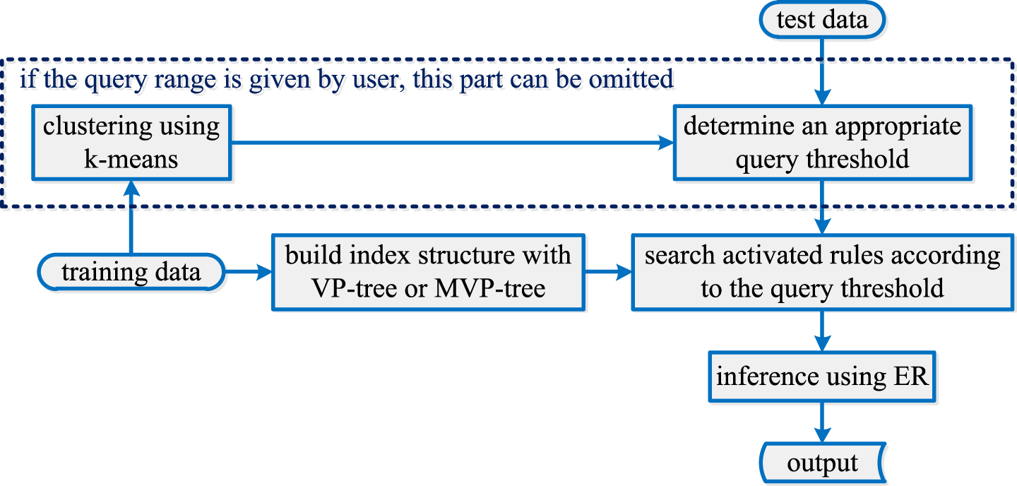
VP-EBRB and MVP-EBRB inference process.

Of course, if you can determine the value of query threshold, then the above steps can be omitted when searching neighbor rules since the k-means algorithm is an iterative method. Its computational complexity is roughly bounded by O (tdkN), where N is the number of data objects, d is the data dimension, k is the number of clusters to be formed, and t is the number of iterations before termination.

Then we can construct the index structure for EBRB based on VP-tree and MVP-tree. Since the belief degree distributions of antecedent attributes in EBRB rules are actually the probability distributions, the distance of two extended rules R_p and R_q can be calculated as follows: $d (R_{p}, R_{q}) = \sqrt{\sum_{i = 1}^{T} (x_{i}^{p} - x_{i}^{q})^{2}}$ (11) where the ith input in the kth rule is x_i.

After building index structure with VP-tree or MVP-tree, we can retrieve the rules which are within a specified distance of a given input data. Those retrieved rules will be visited and used to calculate each rule’s activation weight. Finally, the activated rules are aggregated using the ER algorithm as the inference engine to get the final reasoning result.

5 Case studies

5.1 Function regression

The authors in [28] exploited a nonlinear function to validate the efficiency of BK-EBRB. The same tests were emulated to validate the reasoning performance and efficiency of the VP-EBRB and MVP-EBRB compared with Liu-ERBB and BK-EBRB. The nonlinear function is given below: $f (x) = x sin (x^{2}), 0 \leq x \leq 3$ (12)

We select 500 numbers from the range of values for x evenly as the training data to generate Liu-EBRB, BK-EBRB, VP-EBRB and MVP-EBRB systems. x is the antecedent attribute with seven referential values {0, 0.5, 1.0, 1.5, 2.0, 2.5, 3.0} and the function value f (x) is the consequent. The number of the degrees of consequent is five and the corresponding utility values are {-2.5, - 1.0, 1.0, 2.0.3.0}. The query threshold is set to be 0.01, so there is no need to use k-means clustering algorithm here. It is worth nothing that the distance of two rules in this experiment is calculated with the formula in [28]. The test data is the 1000 numbers chosen from the range of values for x evenly.

The function regression results are shown in Fig. 2. For the same query threshold, BK-EBRB, VP-EBRB and MVP-EBBR will retrieve the same rules, so the inference results of BK-EBRB, VP-EBRB and MVP-EBRB are represented as one line in Fig. 2. From the Fig. 2, we can see that there is a great difference between the simulated output received from Liu-EBRB system and the observed output calculated by nonlinear function f (x). The difference between the simulated output received from BK-EBRB, VP-EBRB and MVP-EBRB systems and the observed output calculated by nonlinear function f (x) is small. Therefore we can have the conclusion that the BK-EBRB, VP-EBRB and MVP-EBRB systems can fit nonlinear function f (x) better than Liu-EBRB.

Fig.2

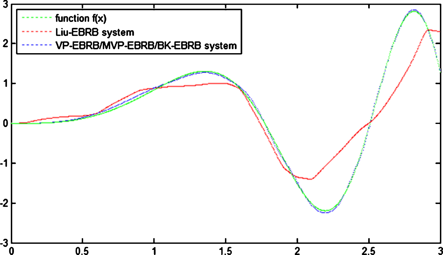
Function regression result.

By comparing the complexity of building systems for Liu-EBRB, BK-EBRB, VP-EBRB and MVP-EBBR, it can be seen from Table 1 that BK-EBRB, VP-EBRB and MVP-EBRB have higher complexity due to the construction of the index structure. However, BK-EBRB, VP-EBRB and MVP-EBRB can visit neighbor belief rules efficiently with lower complexity. Table 2 summarizes the comparison results of the Liu-EBRB, BK-EBRB, VP-EBRB and MVP-EBRB systems. Algorithms are measured regarding to: (1) MSE: the mean squared error between the simulated output and the observed output; (2) RT: the running time of algorithm including the time of building system (BST) and the time of inference procedure (IPT); (3) VR: the total number of rules visited in the calculation of each rule’s activation weight. Compared with Liu-EBRB, VP-EBRB and MVP-EBRB require less time for inference procedure in that the proposed rule activation method only visits partial rules instead of traversing all rules to calculate each rule’s activation weight. Most importantly, as Table 2 illustrates, the MSE of VP-EBRB and MVP-EBRB is smaller than that of Liu-EBRB system. While compared with BK-EBRB, even the MSE of BK-EBRB is the same with VP-EBRB and MVP-EBRB, VP-EBRB and MVP-EBRB need less running time and visit less rules. So it is inferred that VP-EBRB and MVP-EBRB are more efficient.

Table 1

Comparison of the complexity for the Liu-EBRB, VP-EBRB and MVP-EBRB

Complexity	Liu-EBRB	BK-EBRB	VP-EBRB (without k-means)	MVP-EBRB (without k-means)
Build system	n	n log ₂n	n log ₂n	n log _mn (m ≥ 2)
Visit rules	n	n^α0 ≤ α ≤ 1)	log ₂n	far less than n

Table 2

Comparison of the Liu-EBRB, VP-EBRB and MVP-EBRB

	MSE	RT	BST	IPT	VR
Liu-EBRB	0.296986	0.089	0.042	0.047	500000
BK-EBRB	0.000814	0.095	0.071	0.024	34792
VP-EBRB	0.000814	0.065	0.062	0.003	14801
MVP-EBRB	0.000814	0.070	0.061	0.009	14988

Compared with VP-EBRB, there are additional two parameters k and p in the MVP-EBBR. We try to see the effects of parameters k and p of MVP-tree on the search performance of MVP-EBRB systems. Figure 3 shows the results for the MVP-EBRB systems that have different values for the parameter k from 2 to 10 and the same value for the parameter p. Figure 4 shows the results for the MVP-EBRB systems that have different values for the parameter p from 2 to 10 and the same value for the parameter k. The horizontal axis is the total number of visited rules while the vertical axis denotes the value of k or p. In all EBRB systems, the parameters m and r are the same. It can be seen from Fig. 3 that the increase of the parameter k can reduce the number of the total visited rules and improve the search performance of MVP-EBRB systems. However, we can see from Fig. 4 that the change of the parameter p has little influence on the search performance of MVP-EBRB systems.

Fig.3

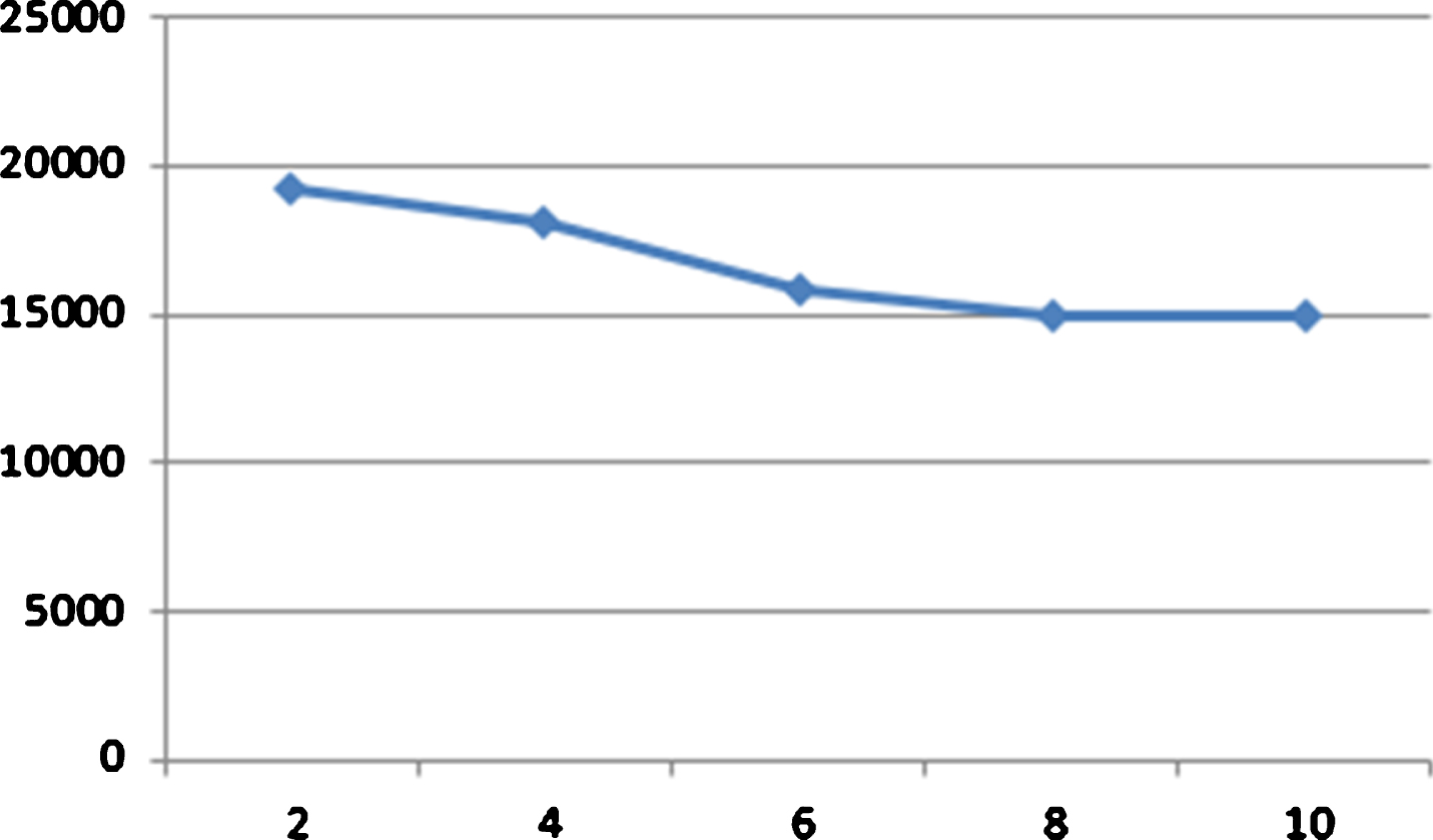
Performance of MVP-EBRB with different k.

Fig.4

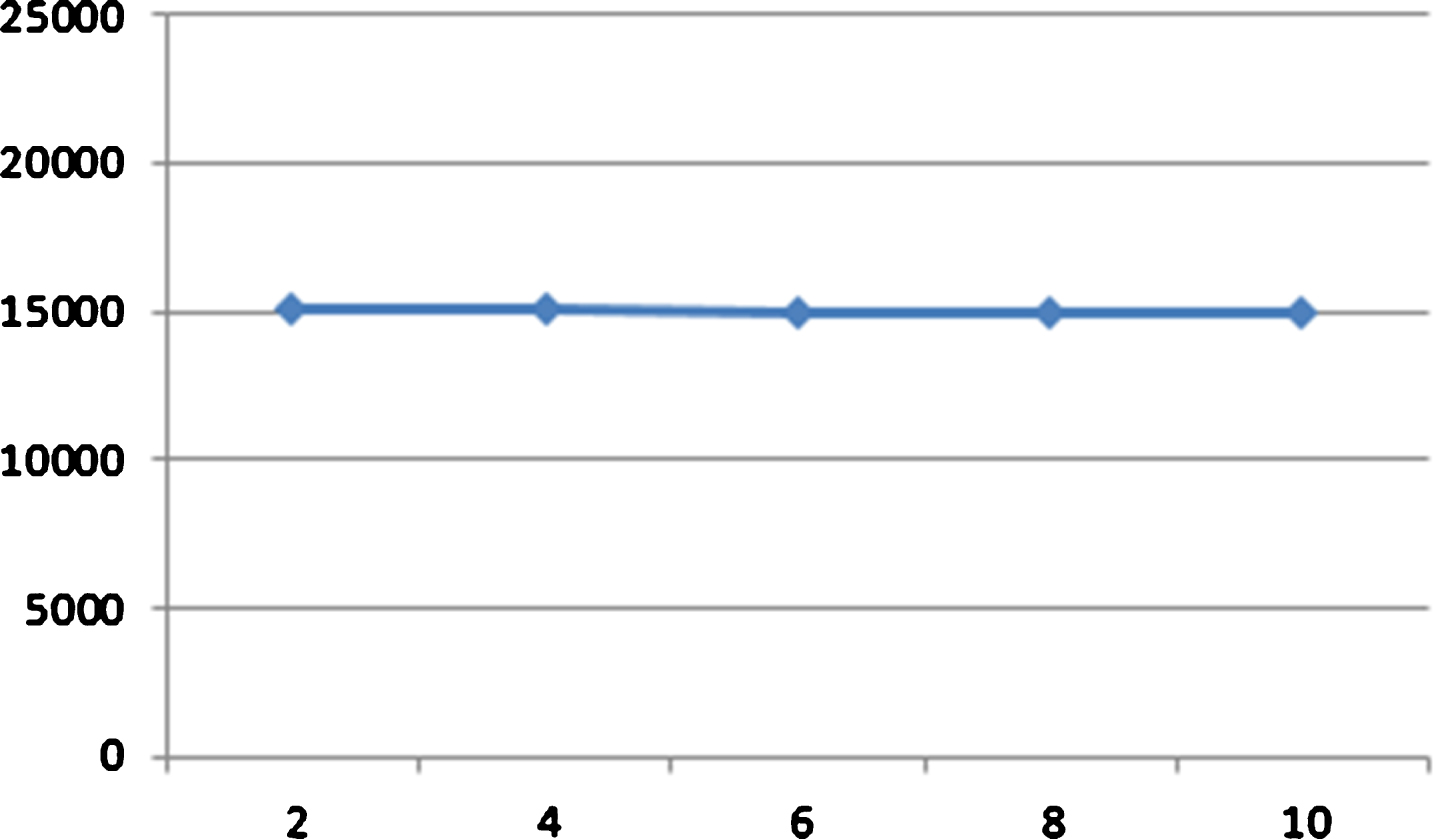
Performance of MVP-EBRB with different p.

5.2 Classification datasets

The first case study is under the premise of the given query threshold. However, it is difficult to determine the value of query threshold in many cases. If the query threshold is too large, it is useless to build index structure on belief rules with VP-tree or MVP-tree since all rules will be visited. However, too small query threshold will cause the problem that no rules are activated because the number of queried rules is zero. Once no rules are activated, the corresponding input data cannot be inferenced with EBRB inference methodology. To show the effect of the query threshold on VP-EBRB or MVP-EBRB, we built VP-EBRB systems on iris dataset using different specified query thresholds. The experimental results are shown in Figs. 5 and 6. In Fig. 5, the vertical axis is the value of query threshold while the horizontal axis denotes the total number of rules visited when calculating each rule’s activation weight. In Fig. 6, the vertical axis is the value of query threshold while the horizontal axis denotes the number of input data that cannot be inferenced as no rules are activated. We can see from Fig. 5 that with the decrease of the value of query threshold, the number of visited rules will be decreased. As Fig. 6 illustrates, with the decrease of the value of query threshold, the number of input data which cannot be inferenced will be increase from zero. That is to say, although small query threshold can reduce visited rules greatly, it can also cause no activated rules problem. So, it is needed to select an appropriate query threshold, which can reduce the visited rules as much as possible and avoid the issue of no activated rules simultaneously.

Fig.5

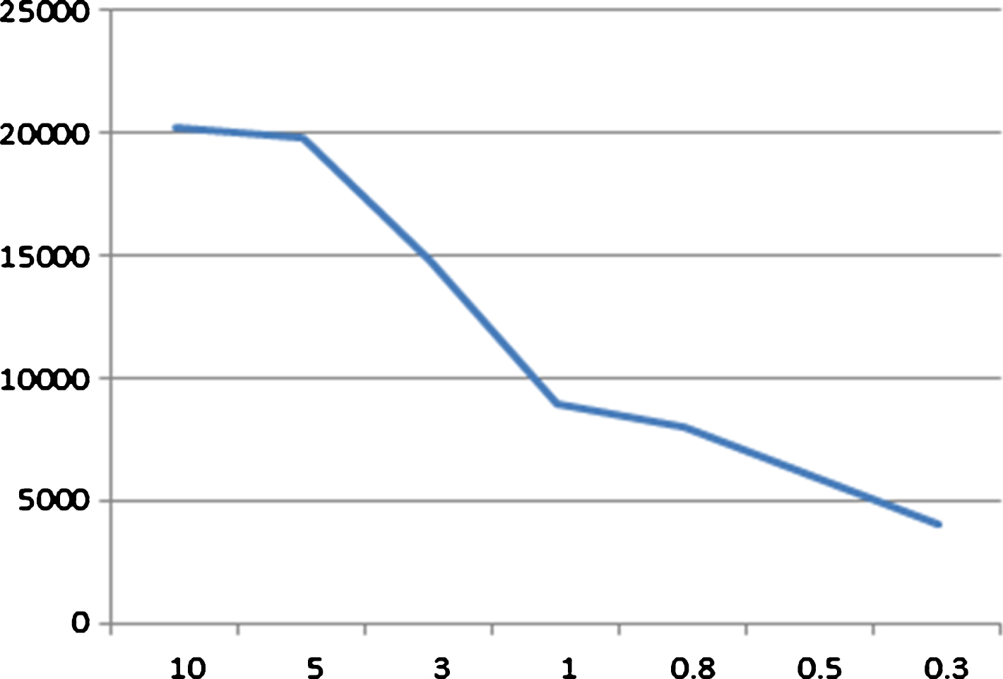
Number of visited rules of VP-EBRB systems.

Fig.6

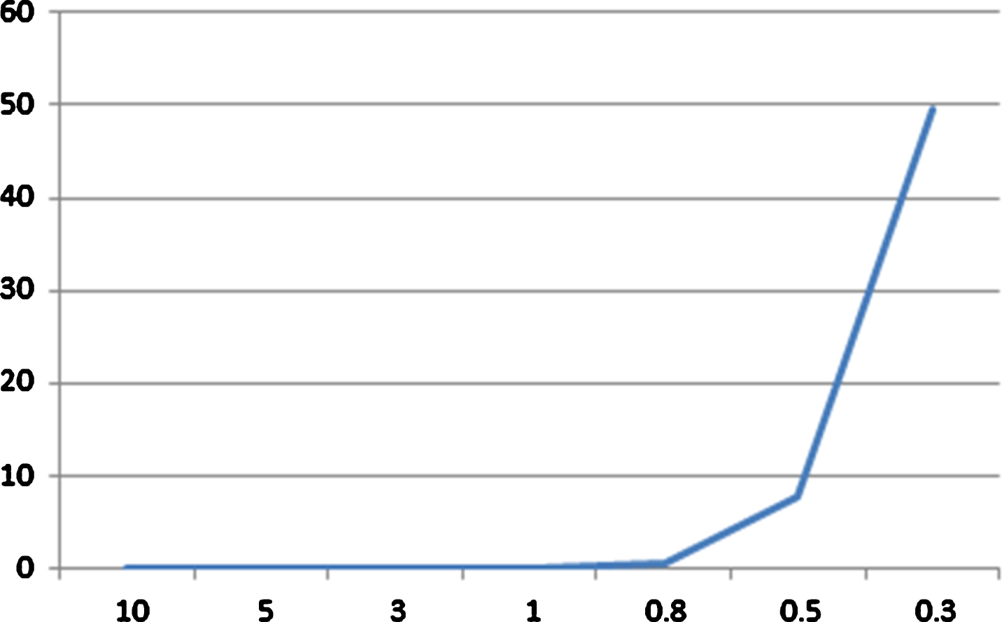
Number of failed tests of VP-EBRB systems.

To validate the efficiency of the proposed selecting the query threshold based on k-means clustering algorithm method, seven benchmark datasets were collected from the UC Irvine Machine Learning Repository [16]. Each dataset was randomized by permuting its samples in order to perform a series of ten 10-fold cross validation tests for VP-EBRB and MVP-EBRB systems. The results about these datasets were measured with (1) Accuracy: the percentage of classes correctly classified from the total samples; (2) VRR: the percentage of rules visited in the inference process from the total rules; (3) Failed: the number of tests where the method could not activate any rules. As Table 3 illustrates, compared with some existing approaches from [26], VP-EBRB and MVP-EBRB systems with k-means clustering algorithm can visit less rules when calculating each rule’s activation weight without causing the no activated rules problem. This is mainly because the proposed rule activation method is based on VP-tree and MVP-tree, which can cut down the number of visited rules and integrate crucial rules to weaken the influence of inconsistent data with appropriate query thresholds selected by k-means algorithm.

Table 3

Comparison with existing methods from [26]

	Aspects	Transfusion	Iris	Seeds	Ecoli	Yeast	Glass	Pima
DRA+WA	Accuracy	76.55	95.63	92.14	83.75	54.15	70.26	71.34
	VRR	100	100	100	100	100	100	100
	Failed	0	0	0	0	0	0	0
DRA+ER	Accuracy	76.57	95.50	92.02	83.76	54.13	69.65	71.44
	VRR	100	100	100	100	100	100	100
	Failed	0	0	0	0	0	0	0
Liu-EBRB	Accuracy	76.14	95.33	91.33	81.16	45.61	67.85	73.39
	VRR	100	100	100	100	100	100	100
	Failed	0	0	0	1	0	3.35	0
VP-EBRB	Accuracy	77.33	95.13	92.57	84.87	58.15	71.75	71.89
	VRR	16.69	39.43	33.76	44.69	40.43	57.13	26.04
	Failed	0	0	0	0	0	1	0
MVP-EBRB	Accuracy	80.36	95.87	92.38	85.61	57.49	72.06	72.59
	VRR	42.63	78.60	81.88	51.18	41.76	84.54	69.52
	Failed	0	0	0	1	0	2	0

6 Conclusion

A new rule activation method based on VP-tree and MVP-tree for the EBRB was proposed in this paper to solve the problem that all belief rules will be visited to calculate each rule’s activation weight in rule activation procedure since all rules are stored out of order. Besides, the reasoning performance of an EBRB will be lowered because of too many activated rules. The proposed optimization method builds index structure on belief rules with the VP-tree or MVP-tree to reduce the number of visited rules. More representative and fewer rules can be retrieved using a suitable query threshold and be aggregated in inference procedure. The query threshold has great impact on the performance of VP-EBRB and MVP-EBRB. Small query threshold can reduce the number of visited rules, but too large query threshold is likely to cause the no activated rules issue. It is worth nothing that the query threshold can be given directly or selected by the proposed clustering approach based on k-means algorithm to avoid the no activated rules issue. Note that the proposed method not only cuts down the reasoning time, but also opens the possibility of achieving better reasoning performance. Moreover, the proposed optimization method has good scalability, which can be combined with any other decision models with belief degree distribution frameworks.

In the case of function regression, this paper has validated that the proposed rule activation method can improve the EBRB systems’ reasoning performance. And the case of data with numerous classes has demonstrated the importance of query threshold and the effectiveness of using k-means clustering algorithm to select appropriate query thresholds. Nevertheless, it needs to specify the number of clusters in advance and it is an iterative algorithm. And the parameters in MVP-tree will also influence the reasoning performance of systems and had better be learned with optimization algorithms. Further research should be carried out to select better methods to address the no activated rules issue.

Footnotes

Acknowledgments

This research was supported by the National Natural Science Foundation of China (Nos. 71371053, 71501047, and 61773123) and the Natural Science Foundation of Fujian Province, China (No. 2015J01248).

References

Zadeh

L.A.

, Fuzzy sets, Information and Control8(3) (1965), 338–353.

Dempster

A.P.

, A generalization of Bayesian inference, Journal of the Royal Statistical Society, Series B (Methodological) (1968), 205–247.

Shafer

, A mathematical theory of evidence, Princeton: Princeton University Press, 1976.

Wang

C.L.

and Yoon

K.S.

, Multiple attribute decision making: Methods and applications, Berlin: Spring-verlag, 1981.

Uhlmann

J.K.

, Satisfying general proximity/similarity queries with metric trees, Information Processing Letters40(4) (1991), 175–179.

Yianilos

P.N.

, Data structures and algorithms for nearest neighbor search in general metric spaces, ACM-SIAM Symposium on Discrete Algorithms (1993), 311–321.

Sun

, Robust reasoning: Integrating rule-based and similarity-based reasoning, Artificial Intelligence75(2) (1995), 241–295.

Bozkaya

and Ozsoyoglu

, Indexing large metric spaces for similarity search queries, ACM Transactions on Database Systems24(3) (1999), 361–404.

Wang

Z.Q.

, Gan

G.H.

and Cheng

Q.M.

, Image retrieval based on high-dimensional index structure for metric spaces VP-tree and MVP-tree, Computer Engineering and Applications40(36) (2004), 41–44.

10.

Yang

J.B.

, Liu

, Wang

, Sii

H.S.

and Wang

H.W.

, Belief rule-base inference methodology using the evidential reasoning approach-RIMER, IEEE Transactions on Systems, Man and Cybernetics Part A-Systems and Humans36(2) (2006), 266–285.

11.

Yang

J.B.

, Liu

, Xu

D.L.

, Wang

and Wang

, Optimization models for training belief-rule-based systems, IEEE Transactions on Systems, Man and Cybernetics Part A-Systems and Humans37(4) (2007), 569–585.

12.

D.L.

, Liu

, Yang

J.B.

, Liu

G.P.

, Wang

, Jenkinson

and Ren

, Inference and learning methodology of belief-rule-based expert system for pipeline leak detection, Expert Systems with Applications32(1) (2007), 103–113.

13.

Zhou

Z.J.

, Hu

C.H.

, Yang

J.B.

, Xu

D.L.

and Zhou

D.H.

, Online updating belief rule based system for pipeline leak detection under expert intervention, Expert Systems with Applications36(4) (2009), 7700–7709.

14.

Liu

, Yang

J.B.

, Ruan

, Martinez

and Wang

L.J.

, Self-tuning of fuzzy belief rule bases for engineering system safety analysis, Annals of Operations Research163(1) (2008), 143–168.

15.

Liu

, Martinez

, Wang

, Rodriquez

R.M.

and Novozhilov

, Computing with words in risk assessment, International Journal of Computational Intelligence Systems3(4) (2010), 396–419.

16.

Frank

and Asuncion

, UCI machine learning repository. School Comput Sci, Univ California, Los Angeles, CA, USA, 2010. [Online], Available: http://archive.ics.uci.edu/ml

17.

Zhou

Z.J.

, Hu

C.H.

, Yang

J.J.

, Xu

D.L.

and Zhou

D.H.

, Online updating belief-rule based systems using the RIMER approach, IEEE Transactions on Systems, Man and Cybernetics Part A-Systems and Humans41(6) (2011), 1225–1243.

18.

Chen

Y.W.

, Yang

J.B.

, Xu

D.L.

, Zhou

Z.J.

and Tanga

D.W.

, Inference analysis and adaptive training for belief rule based systems, Expert Systems with Applications38(10) (2011), 12845–12860.

19.

Liu

, Martinez

, Calzada

and Wang

, A novel belief rule base representation, generation and its inference methodology, Knowledge-Based Systems53 (2013), 129–141.

20.

, Yang

L.H.

, Fu

Y.G.

, Wu

Y.J.

and Gong

X.T.

, Parameter training approach based on variable particle swarm optimization for belief rule base, Journal of Computer Applications34(8) (2014), 2161–2165.

21.

R.Y.

, Yang

L.H.

and Fu

Y.G.

, Data driven construction and inference methodology of belief rule-base, Journal of Computer Applications34(8) (2014), 2155–2160.

22.

Liu

S.G.

and Wei

Y.W.

, Fast nearest neighbor searching based on improved VP-tree, Pattern Recognition Letters60 (2015), 8–15.

23.

Chang

L.L.

, Sun

J.B.

, Jiang

and Li

M.J.

, Parameter learning for the belief rule base system in the residual life probability prediction of metalized film capacitor, Knowledge-Based Systems73(1) (2015), 69–80.

24.

Wang

H.J.

, Yang

L.H.

, Fu

Y.G.

, Wu

Y.J.

and Gong

X.T.

, Differential evolutionary algorithm for parameter training of belief rule base under expert intervention, Computer Science42(5) (2015), 88–93.

25.

Jin

L.Q.

, Liu

, Xu

and Fang

, A novel rule base representation and its inference method using the evidential reasoning approach, Knowledge-Based Systems87 (2015), 80–91.

26.

Calzada

, Liu

, Wang

and Anil

, A new dynamic rule activation method for extended belief rule-based systems, IEEE Transactions on Knowledge and Data Engineering7(4) (2015), 880–888.

27.

Ball

and Hall

, A novel method of data analysis and pattern classification. California: Technical rept. NTIS AD 699616. Stanford Research Institute, 1965.

28.

, Yang

L.H.

, Fu

Y.G.

and Yu

R.Y.

, Structure optimization framework of extended belief rule based on BK-Tree, Journal of Frontiers of Computer Science and Technology10(2) (2016), 257–267.

29.

Yang

, Fu

, Chen

Y.W.

, Xu

D.L.

and Yang

S.L.

, A belief rule based expert system for predicting consumer preference in new product development, Knowledge-Based Systems94 (2016), 338–353.

30.

Burkhard

W.A.

and Keller

R.M.

, Some approaches to best-match file searching, Communications of the ACM16(4) (1973), 230–236.