An integrated cellular manufacturing system with type-2 fuzzy variables: Three tuned meta-heuristic algorithms

Abstract

In this paper, a mixed-integer non-linear programming model has been proposed to design an integrated cellular manufacturing system with type-2 fuzzy parameters. The integrated cellular manufacturing system consists of the following elements: cell formation, cellular layout and operator and tool assignment. One of the important features of the proposed model is considering total expected cost criteria to operator assignment. Tool costs, inter and intra cell movement costs and machine constant costs are type-2 fuzzy variables. In order to defuzzification of parameters the critical value (CV)-based reduction method is used to reduce type-2 fuzzy variables into type-1 fuzzy variables and finally the centroid defuzzification method defuzzifies fuzzy costs to crisp numbers of the costs. Furthermore, to solve a small-sized numerical example, the Branch and Bound algorithm with the Lingo software has been used. Because of NP-hardness of the model for large-sized problems and no exist benchmark to validate the performance of the proposed model, three tuned meta-heuristic algorithms (i.e., particle swarm optimization, differential evolution and fire fly) are presented too. The results show that the particle swarm optimization algorithm has better statistically performances in most problems.

Keywords

Cellular manufacturing system design fuzzy type-2 defuzzification tuned meta-heuristic methods

1 Introduction

A cellular manufacturing system (CMS) prepares the advantages, such as less handling time and cost, Improvement in setup time and work-in-process inventories, increase capacity of the machines, better Responsiveness. There are four problems in the CMS design consisting of a cell formation problem (CFP), group layout problem (GLP), group scheduling problem (GSP), resource assignment problem (RAP) [54]. The term ‘RAP’ refers to the assignment of tools and operators. There is a large number of the published studies (e.g., Min and Shin [26], Norman et al. [30], Mahdavi et al. [21], Mahdavi et al. [23], Süer and Bera [45], Suresh et al. [48], Slomp et al. [42], Aryanezhad et al. [2], Hamedi et al. [11], Mehdizadeh and Rahimi [25] and Bagheri and Bashiri [4]) that described the operator assignment problem in the CMS design. There are relatively few historical studies in the area of tool assignment problems in the CMS design (e.g., Jain et al. [13] and Selim et al. [39]). There is a relatively few literature reviews (e.g., AL-Ahmari and Alharbi [1] and Selim et al. [39]) that are concerned with operator and tool assignment problems in the CMS design simultaneously.

A two-phase procedure for a CFP by tabu search was proposed in Logendran et al. [19]. Vakharia and Chang [53] considered some of important features in a CMS design, such as operation sequence, replication of machines, movement of material between cells (i.e., inter-cell movement) and number of machines in each cell (i.e., cell size). cell formation (CF) in multi-period planning horizon is called dynamic CF, which considered by numerous researchers, such as Balakrishnan and Cheng [5], Deljoo et al. [7], Mungwattana [28], Safaei et al. [35] and Tavakkoli-Moghaddam et al. [49] with characteristics, such as meta-heuristics and fuzzy conditions. In Rafiei and Ghodsi [34], a hybrid meta-heuristic algorithm based on ant colony optimization (ACO) and genetic algorithm (GA) was developed to solve a bi-objective mathematical formulation for the dynamic CFP. The objectives were to (1) minimize the DCFP costs and (2) maximize the labor utilization. Majazi Dalfard [24] presented a new idea consist of more material flow in shorter distance for minimization of average length of intra and intercellular movements and number of intra and inter-cellular movements and solved by simulated annealing (SA). There have been some studies assumed the cell formation and layout problems simultaneously, such as Heragu and Kakuturi [12] and other researchers extended its such as Chen and Cao [6], Dimopoulos and Zalzala [8], Kia et al. [17], Kia et al. [15], Kia et al. [16], Mahdavi et al. [21], Safaei and Tavakkoli-Moghaddam [37], Solimanpur et al. [43] and Tavakkoli-Moghaddamet al. [51].

A resource assignment problem (RAP) generally consists of labor and tool assignment problems. A multiple objective model for cell formation and labor assignment, simultaneously developed by Min and Shin [26]. In Norman et al. [30] a mixed-integer programming (MIP) model for cell formation with worker assignment with human skills criteria was presented. Cell formation and production planning, worker assignment with characteristics (e.g., worker hiring, firing and salary costs in a dynamic MIP model was presented by Mahdavi et al. [21]. Mahdavi et al. [23] developed a ɛ-constraint method to solve a bi-objective mathematical model for a cellular manufacturing system design considering worker interest concept. An integrated mathematical model for cell formation considering tool and minimization of the tools cost and machines cost was developed in Jain et al. [13].

Selim et al. [39] developed a mathematical model for the CFP with tool and worker assignments, which minimizes the objective function consisting of the fixed and variable costs of machines, tooling cost, handling cost and worker training cost. AL-Ahmari and Alharbi [1] developed a mathematical model to the CMS design for CF and tool and worker assignments under the alternate process plans situation. A mathematical model to the CF and layout problems with operator assignment was developed by Bagheri and Bashiri [4], and the LP-metric approach to obtain preferred solutions was applied. Dynamic CF and group layout problems with operator assignment and machine duplication in an integrated mathematical model was presented by Mehdizadeh and Rahimi [25].

Safaei et al. [36] developed a fuzzy programming-based approach to solve the DCFP, in which there are fuzzy numbers as coefficients in the objective function and the technological matrix. Tavakkoli-Moghaddam et al. [50] presented a fuzzy linear MIP model to design cellular manufacturing systems with fuzzy part demands and product mix changeable under a multi-period planning horizon. Azadeh et al. [3] illustrated the use of MCDM methods to identify optimal scenario selection in a simulation model, and showed how to identify the optimum operator layout with respect to a cellular condition. Fazlollahtabar et al. [9] concerned with both time and cost optimization in an automated manufacturing system, in which material handling is carried out by automated guided vehicles and robots for the system.

An integrated method was proposed by obtaining data from simulation and utilizing fuzzy AHP and TOPSIS methods to solve this problem. García [10] proposed two general methods to handle uncertainties in the right hand side parameters of a linear programming (LP) model by means of interval type-2 fuzzy sets (IT-2FS), and solved by a type-reduction method and a pre-defuzzified α-cut approach strategies. Qin et al. [33] proposed three types of critical values (CVs) for a regular fuzzy variable (RFV), and three novel methods of reduction for a type-2 fuzzy variable. In Kundu et al. [18] two fixed charge transportation problems with type-2 fuzzy parameters, which in the first defuzzified values of the type-2 fuzzy cost parameters by critical value (CV)-based reduction methods to type-1 fuzzy variables, and then centroid method was used for complete defuzzification. In this research, the cell formation, group layout, operator assignment and tool assignment problems are modeled simultaneously, that focused on a new Criteria to the operator assignment that called ‘total expected cost’.

In this paper, tool costs, inter and intra-cell movement costs and machine constant costs are type-2 fuzzy variables. In order to defuzzification of parameters, the critical value (CV)-based reduction method is used to reduce type-2 fuzzy variables into type-1 fuzzy variables and finally the centroid defuzzification method defuzzifies fuzzy costs to crisp numbers of the costs. Additionally, the branch-and-bound algorithm with the Lingo software is used to solve a numerical example. Up to now, the previous studies have used a branch-and-bound algorithm embedded in Lingo software (e.g., AL-Ahmari and Alharbi [1], Mahdavi et al. [22], Kia et al. [17], Bagheri and Bashiri [4] and Mahdavi et al. [21]). Because of NP-hardness of the model for large-sized problems and no existing benchmark to validate the performance of the proposed model, three tuned meta-heuristic algorithms are presented too. In this paper, we use synchronous servicing to man and machine relationships and total expected cost to operator assignment. The number of machines to be assigned operator is given by: $N = \frac{l + m}{l + w}$ where,

N = number of machines the operator is assigned

l = Total operator servicing time per machine consist of loading and unloading time

M = Total machine running time

w = walking time to the next machine

k₁= Operator rate per unit of time

k₂= Cost of machine per unit of time

If N is a fraction then N₁ ≤ N ≤ N₂

N₁ is the lowest number and N₂ = N₁ + 1

The total expected cost for N₁ machine and N₂ machine are determined as follows: $\begin{matrix} T . E . C_{N 1} & = & \frac{k_{1} . (l + m) + N_{1} . k_{2} . (l + m)}{N_{1}} \\ T . E . C_{N 2} & = & \frac{k_{1} . N_{2} (l + w) + k_{2} \cdot N_{2} . N_{2} . (l + w)}{N_{2}} \end{matrix}$

The number of machines assigned to operators has the minimum total expected cost [29]. The structure of the rest of the paper is organized as follows. In the next section presents Problem description. Fundamental concepts of the type-2 fuzzy set is followed in Section 3. In Section 4, a numerical example under the type-2 fuzzy condition is presented. The solution algorithms is described in Section 5. Data generating, tuning parameters and computational results is reported in Section 6. Finally, in Section 7 concludes the paper.

2 Problem description

In this section, the integrated problem is formulated as a mixed-integer nonlinear programming (MINLP) model based on cell formation, inter cell-layout, resource assignment under the following assumptions with the total expected cost criteria simultaneously.

2.1 Assumptions

Each part type has a number of operations that must be processed based the route sheet ofparts.

Any operation in one part can be done on different machines with different processing times.

Demand for each part type is known.

Capability and time capacity of each machine are precise and constant over the planning horizon.

Capability and available time of each operator type are known.

Maximum number of cells is given and fixed.

Capability of each operator type for processing each part on each corresponding machine type and each tool type are known.

All machine types are supposed to be multi-purposed ones.

Constant and variable cost of each machine type are known.

Parts move in a batch inside and outside the cells.

Cost of intra-cell and inter-cell movement depends on their average length and number of intra-cell and inter-cell movements. Average length of this movement is equal to distance between centers of cells.

Cost of machine type m for each unit time is known.

Rate of operator type w for each unit time is known.

Number of slots needed by each tool type and Number of slots available at each machine type are given and fixed.

Total operator loading and unloading time per each machine type to process each type operation on each type part using each tool type are given and fixed.

Number of cell candidate locations is constant over planning horizon.

All machine types are supposed to be identical.

Tool life is known.

2.2 Notations

Indices:

p Index for part types (p = 1, …, P) j Index for operation type (j = 1, …, J) m Index for machine type (m = 1, …, M) c Index for manufacturing cell (c = 1, …, C) l Index for location (l = 1, …, L) t Index for tools (T = 1, …, T) w Index for operator (w = 1, …, W)

2.2.1 Input parameters

t_jpmtw Machining time needed to process operation j on parts type of p on machine type m using tool t by operator w r_jpmtw Equals to 1, if operation j on parts type of p is done on machine type m using tool t by operator w; 0, otherwise $γ_{p}^{inter}$ Inter cell movement cost per part type p per unit of distance $γ_{p}^{intra}$ Intra cell movement cost per part type p per unit of distance D_p Demand for part type p T_m Time capacity of one unit machine of type m T_w Time capacity of operator of type w UB_c Upper bound for cell size in terms of the number of machines d_cc′ Average distance between candid places belonging to cell c if (c=c′) $t_{jpmtw}^{'}$ Total operator servicing (loading and unloading) time per machine type m to process operation j on parts type of p using tool t by operator w $t_{jpmtw}^{''}$ Normal walking time to the next machine ∥K_jpmtw Operating cost of operation j on parts type of p is done on machine type m using tool t by operator w F_cc′ Equals to 1, if c ≠ c′; 0, if c = c′ φ_m Constant cost of machine type m Q_t Number of slots needed by tool t TQ_m Number of slots available at machine m β_m Cost of machine type m for each unit time α_w Cost of operator type w for each unit time λ_t Cost of tool t $B_{p}^{inter}$ Batch size for inter-cell movements of part p $B_{p}^{intra}$ Batch size for intra-cell movements of part p TL_t Tool life of tool t

2.2.2 Decision variables

x_jpmctw Equals to 1, if operation j of part type p is done on machine type m in cell c using tool t by operator; 0, otherwise P_tm Number of available tool copies for tool t u_jpmc Equals to 1, if operation j of part type p is done on machine type m in cell c; 0, otherwise z_jpm Equals to 1, if operation j of part type p is done on machine type m; 0, otherwise zz_mc Equals to 1, if machine type m is assigned to cell c; 0, otherwise y_cl Equals to 1, if cell c is assigned to location l; 0, otherwise Y1_mw Equals to 1, if machine m is assigned to operator w; 0, otherwise Y2_mw Equals to 1, if machine m is assigned to operator w; 0, otherwise

2.2.3 Auxiliary variables

N_mw Number of machines type m the operator w is assigned N1_mw Lowest whole number of machines type m the operator w is assigned N2_mw Uppermost whole number of machines type m the operator w is assigned T . E . C Total expected cost of production per cycle from one machine T . E . C . greaterthan Total expected cost with N1 machine N2_mw type m the operator w is assigned T . E . C . Total expected cost with N2 machine N2_mw type m the operator w is assigned NN_mwc Number of machines type m the operator w is assigned in cell c

2.3 Mathematical model

By using the above notations, the proposed model is now written by: $\begin{matrix} Min \\ \sum_{j = 1}^{J} \sum_{p = 1}^{P} \sum_{m = 1}^{M} \sum_{c = 1}^{C} \sum_{t = 1}^{T} \sum_{w = 1}^{W} D_{p} K_{jpmtw} x_{jpmctw} \\ + \sum_{j = 1}^{J - 1} \sum_{p = 1}^{P} \sum_{c = 1}^{C} \sum_{c^{'} = 1}^{C} [\frac{D_{p}}{B_{p}^{intra}}] {\tilde{γ}}_{p}^{intra} F_{{cc}^{'}} d_{{cc}^{'}} \end{matrix}$ (1) $(\sum_{m = 1}^{M} u_{j p m c}) (\sum_{m = 1}^{M} u_{j + 1, p m c^{'}}) y_{c l} y_{c' l'}$ (1.2) $\begin{matrix} + \sum_{j = 1}^{J - 1} \sum_{p = 1}^{P} \sum_{c = 1}^{C} \sum_{c^{'} = 1}^{C} [\frac{D_{p}}{B_{p}^{intra}}] {\tilde{γ}}_{p}^{intra} (1 - F_{{cc}^{'}}) \\ d_{{cc}^{'}} (\sum_{m = 1}^{M} u_{jpmc}) (\sum_{m = 1}^{M} u_{j + 1, {pmc}^{'}}) \end{matrix}$ (1.3) $+ \sum_{m}^{M} \sum_{w}^{W} {\tilde{φ}}_{m} (N 1_{mw} Y 2_{mw} + N 2_{mw} Y 1_{mw})$ (1.4) $\begin{matrix} + \\ \sum_{t = 1}^{T} {\tilde{λ}}_{t} \sum_{m = 1}^{M} P_{tm} \end{matrix}$ (1.5)

$\begin{matrix} s . t . \\ \sum_{m}^{M} \sum_{c}^{C} \sum_{t}^{T} \sum_{w}^{W} x_{jpmctw} . r_{jpmtw} = 1 \forall j, p \end{matrix}$ (2) $x_{jpmctw} \leq r_{jpmtw} \forall j, p, m, c, t, w$ (3) $\sum_{m}^{M} \sum_{w}^{W} {NN}_{mwc} \leq {UB}_{c} \forall c$ (4) $u_{jpmc} = z_{jpm} {zz}_{mc} \forall j, p, m, c$ (5) $\begin{matrix} {NN}_{mwc} {zz}_{mc} \\ = N 1_{mw} Y 2_{mw} + N 2_{mw} Y 1_{mw} \forall m, w, c \end{matrix}$ (6) $\begin{matrix} \sum_{j}^{J} \sum_{p}^{P} \sum_{c}^{C} \sum_{t}^{T} D_{p} x_{jpmctw} (t_{jpmtw} + t_{jpmtw}^{'}) \\ \leq T_{w} + MY 1_{mw} \forall m, w \end{matrix}$ (7) $\begin{matrix} \sum_{j}^{J} \sum_{p}^{P} \sum_{c}^{C} \sum_{t}^{T} D_{p} x_{jpmctw} N 2_{mw} t_{jpmtw} \\ \leq T_{w} + MY 2_{mw} \forall m, w \end{matrix}$ (8) $\begin{matrix} \sum_{j}^{J} \sum_{p}^{P} \sum_{c}^{C} \sum_{t}^{T} D_{p} x_{jpmctw} (t_{jpmtw} + t_{jpmtw}^{'}) \\ \leq T_{m} + MY 1_{mw} \forall m, w \end{matrix}$ (9) $\begin{matrix} \sum_{j}^{J} \sum_{p}^{P} \sum_{c}^{C} \sum_{t}^{T} D_{p} x_{jpmctw} N 2_{mw} t_{jpmtw} \\ \leq T_{m} + MY 2_{mw} \forall m, w \end{matrix}$ (10) $\begin{matrix} \frac{(t_{jpmtw}^{'} + t_{jpmtw}) . x_{jpmctw}}{t_{jpmtw}^{'} + t_{jpmtw}^{''}} \\ \leq N 2_{mw} \forall j, p, m, c, t, w \end{matrix}$ (11) $N 2_{mw} = r_{jpmtw} (N 1_{mw} + 1) \forall j, p, m, t, w$ (12) $\begin{matrix} T . E . C . N 1_{mw} = r_{jpmtw} . \\ \frac{((t_{pjmtw}^{'} + t_{pjmtw}) (α_{w} + N 1_{mw} \times β_{m}))}{N 1_{mw}} \\ \forall p, j, m, t, w \end{matrix}$ (13) $\begin{matrix} T . E . C . N 2_{mw} = r_{jpmtw} . \\ ((t_{pjmtw}^{'} + t_{pjmtw}^{''}) (α_{w} + β_{m} \times N 2_{mw})) \\ \forall p, j, m, t, w \end{matrix}$ (14) $\begin{matrix} T . E . C . N 1_{mw} \\ \leq T . E . C . N 2_{mw} + MY 1_{mw} \forall m, w \end{matrix}$ (15) $\begin{matrix} T . E . C . N 2_{mw} \\ \leq T . E . C . N 1_{mw} + MY 2_{mw} \forall m, w \end{matrix}$ (16) $Y 1_{mw} + Y 2_{mw} = 1 \forall m, w$ (17) $\sum_{l = 1}^{L} y_{cl} = 1 \forall c$ (18) $\sum_{c = 1}^{C} y_{cl} \leq 1 \forall l$ (19) $\begin{matrix} \sum_{j}^{J} \sum_{p}^{P} \sum_{c}^{C} \sum_{w}^{W} t_{pjmtw} . x_{jpmctw} \leq {TL}_{t} . P_{tm} \\ \forall t, m \end{matrix}$ (20) $\sum_{t}^{T} Q_{t} P_{tm} \leq {TQ}_{m} \forall t, m$ (21) $\sum_{t}^{T} \sum_{w}^{W} x_{jpmctw} = u_{jpmc} \forall p, j, m, c$ (22) $\begin{matrix} x_{jpmctw}, u_{jpmc}, y_{cl}, Y 1_{mw}, Y 2_{mw}, \\ z_{jpm}, {zz}_{mc} \in {0, 1} \end{matrix}$ (23) $\begin{matrix} N 1_{mw}, N 2_{mw}, {NN}_{mwc}, \\ P_{tm} \geq 0, integer \end{matrix}$ (24)

The objective function of the proposed model consists of five terms. Equation (1.1) is the totalprocessing cost. Equation (1.2) is the sum of inter-cell material handling costs, and Equation (1.3) is the sum of intra-cell material handling costs. Equation (1.4) is the total constant cost of all machines required in all cells. Equation (1.5) ensures that the tooling cost. Constraints (2) and (3) indicates that each part-operation is assigned to one machine and one cell and one tool and one operator. Constraint (4) guarantees the maximum cell size is not violated. Constraint (5) is employed in order to definition of zz_mc. Constraint (6) show the number of machines type m, in which operator w is assigned in cell c. Constraints (7) and (8) ensure that the time available to operator with different cycle times and different number machine is not exceeded. Constraints (9) and (10) guarantee that the capacity of each machine type with different cycle times is not violated.

Constraint (11) determines the number of machines that the operator should be assigned by establishing the uppermost whole number. Constraint (12) determines the lowest whole number of machines type m the operator w is assigned. Equations (13) and (14) determine the cost of production per cycle from one machine in the uppermost whole and the lowest whole number of machines. Constraints (15) and (16) compare the total expected cost for N₁, N₂ machine, and the number of machines assigned with the lowest total expected cost is chosen. Constraint (17) guarantees that either or the uppermost whole and the lowest whole number of machines is assigned to operator. Constraints (18) and (19) ensure that each cell should be assigned to only one candidate location and a location can be opened only for one cell. Constraints (20) determines the tool and machine assignment, the magazine capacity restriction is represented by Constraint (21). Constraint (22) is employed in order to definition of u_jpmc. Constraints (23) identifies binary variables, and Constraints (24) shows the non-negativity decision variables.

2.4 Linearization

The proposed model is a nonlinear integer programming model. We can define some auxiliary variables to linearize these nonlinear terms of the model. In Equations (1.2) and (1.3), a classic strategy for linearization of the product of two variables 0 and 1 is as follows. First, zero-one variables (v_jpcc′) are defined by: $υ_{j p c c'} = (\sum_{m = 1}^{M} u_{j p m c}) (\sum_{m = 1}^{M} u_{j + 1, p m c^{'}})$

Then, two following constraints are added to the model. $\begin{matrix} v_{{jpcc}^{'}} \geq (\sum_{m = 1}^{M} u_{jpmc}) + (\sum_{m = 1}^{M} u_{j + 1, {pmc}^{'}}) - 1 \\ \forall j, p, c, c^{'} \end{matrix}$ (25) $\begin{matrix} v_{{jpcc}^{'}} \leq \frac{1}{2} (\sum_{m = 1}^{M} u_{jpmc} + \sum_{m = 1}^{M} u_{j + 1, {pmc}^{'}}) \\ \forall j, p, c, c^{'} and, {yy}_{c c^{'} {ll}^{'}} = y_{c l} y_{c' l'} \end{matrix}$ (26)

Then, two following constraints are added to the model. $y y_{c c' l l'} \geq y_{c l} + y_{c' l'} - 1 \forall c, c', l, l'$ (27) $y y_{c c' l l'} \geq \frac{1}{2} (y_{c l} + y_{c' l'}) - 1 \forall c, c', l, l'$ (28)

Then, υyy_{jpcc′ ll′} are defined as follows: $υ y y_{j p c c' l l'} = υ_{j p c c'} y y_{c c' l l'}$

Then, the following constraints are added to the model. $υ y y_{j p c c' l l'} \geq υ_{j p c c'} + y y c c' l l' - 1$ (29) $υ y y_{j p c c' l l'} \leq \frac{1}{2} (υ_{j p c c'} + y y c c' l l')$ (30) and $v_{jpcc'} = (\sum_{m=1}^{M} u_{jpmc}) (\sum_{m=1}^{M} u_{j+1,pmc'})$

Then, the following constraints are added to the model. $\begin{matrix} v_{{jpcc}^{'}} \geq (\sum_{m = 1}^{M} u_{jpmc}) + (\sum_{m = 1}^{M} u_{j + 1, {pmc}^{'}}) \\ - 1 \forall j, p, c, c^{'} \end{matrix}$ (31) $\begin{matrix} v_{{jpcc}^{'}} \leq \frac{1}{2} (\sum_{m = 1}^{M} u_{jpmc} + \sum_{m = 1}^{M} u_{j + 1, {pmc}^{'}}) \\ \forall j, p, c, c^{'} \end{matrix}$ (32)

In Equation (1.6), we have: $N 1 Y 2_{mw} = N 1_{mw} Y 2_{mw}$

Then, the following constraints are added to the model. $N 1 Y 2_{mw} \leq N 1_{mw} \forall m, w$ (33) $N 1 Y 2_{mw} \leq MY 2_{mw} \forall m, w$ (34) $\begin{matrix} N 1 Y 2_{mw} - N 1_{mw} \\ \geq M (Y 2_{mw} - 1) \forall m, w \end{matrix}$ (35)

Then, at the other step: N2Y1_mw = N2_mwY1_mw

Then, the following constraints are added to the model. $N 2 Y 1_{mw} \leq N 2_{mw} \forall m, w$ (36) $N 2 Y 1_{mw} \leq MY 1_{mw} \forall m, w$ (37) $N 2 Y 1_{mw} - N 2_{mw} \geq M (Y 1_{mw} - 1) \forall m, w$ (38)

In Equation (5), zzz_jpmc = z_jpmzz_mc

Then, the following constraints are added to the model. ${zzz}_{jpmc} \geq z_{jpm} + {zz}_{mc} - 1 \forall j, p, m, c$ (39) ${zzz}_{jpmc} \leq \frac{1}{2} (z_{jpm} + {zz}_{mc}) \forall j, p, m, c$ (40)

In Equation (6), NNzz_mwc = NN_mwczz_mc

Then, the following constraints are added to the model. $\begin{matrix} {NNzz}_{mwc} \geq {NN}_{mwc} - M (1 - {zz}_{mc}) \\ \forall j, p, m, c \end{matrix}$ (41) $\begin{matrix} {NNzz}_{mwc} \leq {NN}_{mwc} + M (1 - {zz}_{mc}) \\ \forall j, p, m, c \end{matrix}$ (42)

In Equations (8) and (9), xN2_jpmctw = x_jpmctwN2_mw

Then, the following constraints are added to the model, $xN 2_{jpmctw} \leq N 2_{mw} \forall j, p, m, c, t, w$ (43) $xN 2_{jpmctw} \leq {Mx}_{jpmctw} \forall j, p, m, c, t, w$ (44) $\begin{matrix} xN 2_{jpmctw} - N 2_{mw} \geq M (x_{jpmctw} - 1) \\ \forall j, p, m, c, t, w \end{matrix}$ (45) $\begin{matrix} v_{{jpcc}^{'}}, {yy}_{{cc}^{'} {ll}^{'}}, {vyy}_{{jpcc}^{'} {ll}^{'}}, xy 2_{jpmctw}, \\ xy 1_{jpmctw}, {zzz}_{jpmc} \in {0, 1} \\ xY 2 N 1_{jpmctw}, xY 1 N 2_{jpmctw}, N 1 Y 2_{mw}, \\ xN 2_{jpmctw}, N 2 Y 1_{mw}, \\ {NNzz}_{mwc} \geq 0, integer \end{matrix}$ (46)

3 Type-2 fuzzy set

3.1 Fundamental concepts and definitions

Zadeh [56] introduced a type-2 fuzzy set that is a fuzzy set whose membership grades are type-1 fuzzy sets on [0, 1]. A type-2 fuzzy set $\tilde{A}$ is characterized by the membership function $μ_{\tilde{A}} (x, u)$ :

$\begin{matrix} \tilde{A} & = & {((x, u), μ_{\tilde{A}} (x, u)) | \forall x \in X, \\ \forall u \in J_{x} \subseteq [0, 1]} \end{matrix}$ (47) where, $0 \leq μ_{\tilde{A}} (x, u) \leq 1$ is the type-2 membership function and x ∈ X, u ∈ J_x ⊆ [0, 1] is the primary membership. If $μ_{\tilde{A}} (x, u) = 1$ , ∀u ∈ J_x ⊆ [0, 1], then this type-2 fuzzy set is called interval type-2 fuzzy set and interval type-2 membership function. $\tilde{A}$ can also be written by:

$\tilde{A} = μ_{\tilde{A}} (x, u) / (x, u) J_{x} \subseteq [0, 1]$ (48) where smallintsmallintdenotes union over all acceptable x and u. For discrete universes of discourse smallint is replaced by ∑ . The union of all of the primary memberships J_x is called footprint of uncertainty (FOU). For example, FOU of interval type-2 fuzzy set is as follows:

$FOU (\tilde{A}) = ⋃_{x \in X} J_{x}$ (49)

The term type-2 fuzzy variable is used here to refer to a function from the fuzzy possibility space to the set of real numbers. Let (Γ, A, Pos) denote the possibility space and the following definition for a type-2 fuzzy variable $\tilde{ξ}$ which is A map $Γ \mapsto R$ such that for any $t \in R$ the set ${γ \in Γ | \tilde{ξ} (γ) \leq t} \in A$ . The secondary possibility distribution function of $\tilde{ξ}$ indicated by $\tilde{μ_{\tilde{ξ}}} (x)$ is a map from $R to R [0, 1]$ such that $\tilde{μ_{\tilde{ξ}}} (x) = \tilde{Pos} {γ \in Γ | \tilde{ξ} (γ) = x} x \in R$ and the type-2 possibility distribution function described by $μ_{\tilde{ξ}} (x, u)$ is a map from $R \times J_{x}$ to [0, 1] and defined as $μ_{\tilde{ξ}} (x, u) = Pos {\tilde{μ_{\tilde{ξ}}} (x) = u}, (x, u) \in R \times J_{x}$ , J_x ∈ [0, 1] is the domain of $\tilde{μ_{\tilde{ξ}}} (x)$ , i.e., $J_{x} = {u \in [0, 1] | μ_{\tilde{ξ}} (x, u) > 0}$ . J_x denoted the primary possibility of the point x and for a special value of x, say x = x′, $\tilde{μ_{\tilde{ξ}}} (x^{'}) = μ_{\tilde{ξ}} (x^{'}, u)$ gives the secondary possibilities ∀ u ∈ J_x′ [16, 17].

3.2 Regular fuzzy variable

A discrete regular fuzzy variable (RFV), denoted $\tilde{ξ}$ , is characterized by the following possibility distribution: $\tilde{ξ} \sim (\begin{matrix} r_{1} & r_{2} & r_{n} \\ \dots \\ μ_{1} & μ_{2} & μ_{n} \end{matrix})$ where r_i ∈ [0, 1] for i = 1, 2, …, n, μ_i > 0 and max μ_i = 1 for i = 1, 2, …, n . If $\tilde{ξ} = (r_{1}, r_{2}, r_{3}, r_{4})$ with 0 ≤ r₁ < r₂ < r₃ < r₄ ≤ 1, then $\tilde{ξ}$ is a trapezoidal RFV. If $\tilde{ξ} = (r_{1}, r_{2}, r_{3})$ with 0 ≤ r₁ < r₂ < r₃ ≤ 1, then $\tilde{ξ}$ is a triangular RFV [33].

3.3 Critical values (CV) for RFVs

Because of the complexity of the membership function of the type-2 fuzzy set, the CV-based reduction method is proposed to convert a type-2 fuzzy variable into a type-1 fuzzy variable. Let $\tilde{ξ}$ be a regular type-2 fuzzy variable (RFV). The method is to introduce the critical values (CVs) as representing the values for the RFV $\tilde{ξ}$ (i.e., optimistic CV reduction ( ${CV}^{*} [\tilde{ξ}]$ ), pessimistic CV reduction ( ${CV}_{*} [\tilde{ξ}]$ ) and CV reduction ( $CV [\tilde{ξ}]$ ), or and so corresponding type-1 fuzzy variables) that are derived by using these CVs of the secondary possibilities. Sugeno [46] defined three kinds of CVs for an RFV $\tilde{ξ}$ as follows:

The optimistic CV of $\tilde{ξ}$ denoted by ${CV}^{*} [\tilde{ξ}]$ , is defined by: $C V^{*} [\tilde{ξ}] =_{α \in [0, 1]}^{S U P} [α^P o s {\tilde{ξ} \geq α}]$

While the pessimistic CV of $\tilde{ξ}$ denoted by ${CV}_{*} [\tilde{ξ}]$ , is defined by: $C V^{*} [\tilde{ξ}] =_{α \in [0, 1]}^{S U P} [α^N e c {\tilde{ξ} \geq α}]$

When the CV of $\tilde{ξ}$ denoted by $CV [\tilde{ξ}]$ , is defined by: $C V^{*} [\tilde{ξ}] =_{α \in [0, 1]}^{S U P} [α^C r {\tilde{ξ} \geq α}]$

Let $\tilde{ξ} = (r_{1}, r_{2}, r_{3})$ be a triangular RFV. Then, we have the following items [33]:

The optimistic CV of $\tilde{ξ}$ is ${CV}^{*} [\tilde{ξ}] = r_{3} / (1 + r_{3} - r_{2}),$

The pessimistic CV of $\tilde{ξ}$ is ${CV}_{*} [\tilde{ξ}] = r_{2} / (1 + r_{2} - r_{1}),$

The CV of $\tilde{ξ}$ is $CV [\tilde{ξ}] = {\begin{matrix} \frac{2 r_{2} - r_{1}}{1 + 2 (r_{2} - r_{1})} & r_{2} > \frac{1}{2} \\ \frac{r_{3}}{1 + 2 (r_{3} - r_{2})} & r_{2} \leq \frac{1}{2} \end{matrix}$

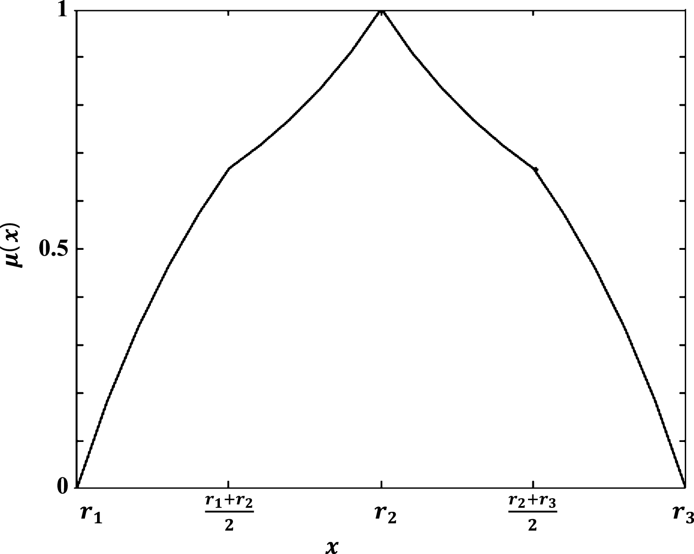
Suppose ξ₁, ξ₂ and ξ₃ be the reduction of $\tilde{ξ}$ obtained by the optimistic CV reduction, pessimistic CV reduction and CV reduction method, respectively. The possibility distributions of ξ₁, ξ₂ and ξ₃ are shown in Figs. 1 to 3, respectively [33].

Fig.1

The Possibility distribution of ξ₁.

Fig.2

The Possibility distribution of ξ₂.

Fig.3

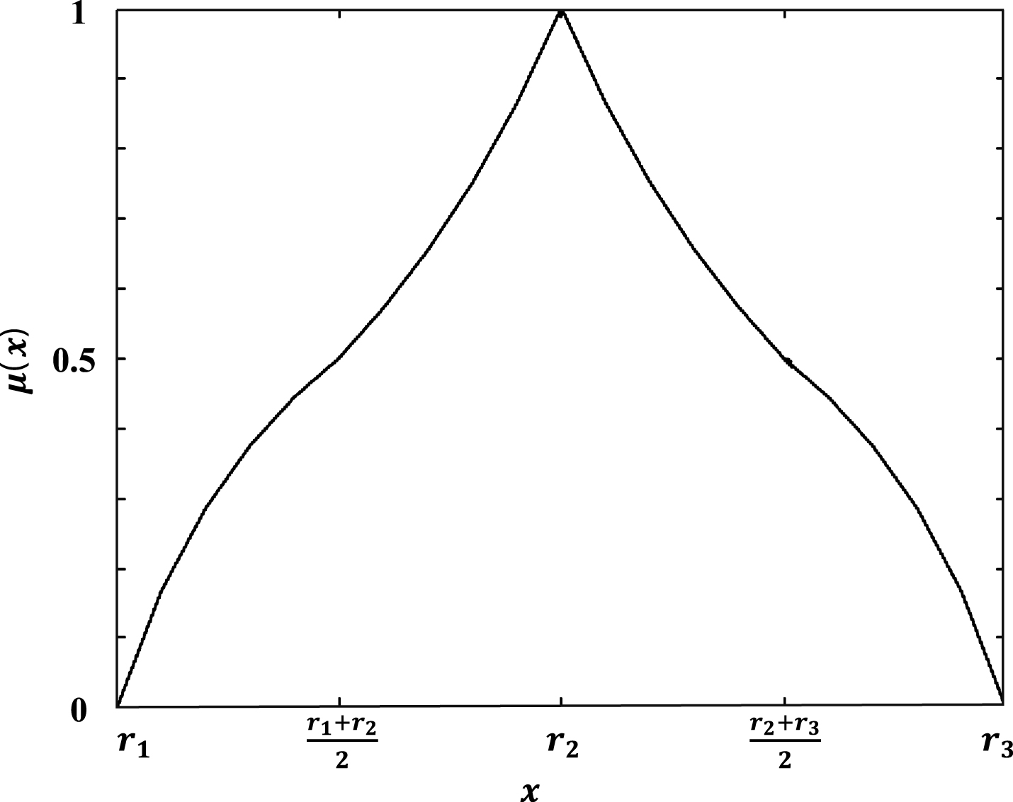
The Possibility distribution of ξ₃.

3.4 Denazification

Kundu et al. [18] presented a defuzzification process of type-2 fuzzy variables. This process included two stages. In the first stage, a CV-based reduction method is used to convert the type-2 fuzzy variables to corresponding type-1 fuzzy variables. In the second stage centroid method is applied to reduction type-1 fuzzy variables to crisp values [47]. Centroid method is the most prevalent and physically appealing of all the defuzzification methods, it is given by the following expression for discrete case. The defuzzification process is shown in Fig. 4. $z^{*} = \frac{\sum_{z} z . μ_{\tilde{A}} (z)}{\sum_{z} μ_{\tilde{A}} (z)}$

Fig.4

Defuzzification process.

4 Numerical example

To solve the proposed model for a small-sized example, a branch-and-bound (B&B) method in using Lingo 9.0 software on a laptop including five Intel (R) core (TM) i5-3230 CPU @ 2.60 GHz and 6 GB RAM. This example consists of three cells, two machines, two parts, two tools, three location and two operators where each part type is assumed to have two operations that must be processed, sequentially. Each operation is able to perform on four alternative machine-tools-operator assignments. The data sets related to the example are shown in Table 1. The machining time and machining cost required for each operation on a machine to part and with a tool by an operator combinations are illustrated in Table 1. ((β_m = (2, 3), ${TQ}_{m} = (7, 7), {\tilde{φ}}_{m} = (3000, 4000), T_{m} = (45, 45)$ and UB = (3, 3, 3)).

Table 1
Typical test problem

Machine Tool Worker P ₁ P ₂

j = 1 j = 2 j = 1 j = 2

M ₁ T ₁ W ₁ W ₂ 0.03,10* 0.03,10 0.03,11 0.03,14

T ₂ W ₁ W ₂ 0.03,9 0.03,11 0.03,12 0.03,12

M ₂ T ₁ W ₁ W ₂ 0.03,14 0.03,15 0.03,10 0.03,12

T ₂ W ₁ W ₂ 0.03,14 0.03,16 0.03,12 0.03,13

D _p 200 100

${\tilde{γ}}_{p}^{inter}$ 10 15

${\tilde{γ}}_{p}^{intra}$ 2 3

Machine	Tool	Worker	P ₁	P ₂
M ₁	T ₁	W ₁ W ₂	0.03,10*	0.03,10	0.03,11	0.03,14
	T ₂	W ₁ W ₂	0.03,9	0.03,11	0.03,12	0.03,12
M ₂	T ₁	W ₁ W ₂	0.03,14	0.03,15	0.03,10	0.03,12
	T ₂	W ₁ W ₂	0.03,14	0.03,16	0.03,12	0.03,13
	D _p		200		100
	${\tilde{γ}}_{p}^{inter}$		10		15
	${\tilde{γ}}_{p}^{intra}$		2		3

*The first figure (0.03) indicates to operation time, and the second figure (10) indicates to operation cost.

The data sets related to the worker information and tools are shown in Table 2. The related parameters of distance between cells are given in Table 3.

Table 2

Typical test problem

Worker	T _w	α _w	$t_{jpmtw}^{'}$	$t_{jpmtw}^{''}$	Tool	Q _t	${\tilde{λ}}_{t}$
W ₁	45	2	0.02	0	t ₁	3	50
W ₂	45	1	0.02	0	t ₂	3	60

Table 3

Information relating to distance between cells for test problem

d _cc′	1	2	3
1	5	10	20
2	10	5	10
3	20	10	5

We assume some of objective function coefficients in the small-sized examples with type-2 fuzzy variables. $\begin{matrix} {\tilde{γ}}_{p}^{intra} = {\begin{matrix} 1 & \tilde{μ} {\tilde{γ}}_{p}^{intra} = (0.4, 0.6, 0.7) \\ 2 & \tilde{μ} {\tilde{γ}}_{p}^{intra} = (0.5, 0.7, 0.8) \\ 3 & \tilde{μ} {\tilde{γ}}_{p}^{intra} = (0.6, 0.8, 0.9) \end{matrix} \\ {\tilde{γ}}_{p}^{intra} = {\begin{matrix} 2 & \tilde{μ} {\tilde{γ}}_{p}^{intra} = (0.4, 0.6, 0.7) \\ 3 & \tilde{μ} {\tilde{γ}}_{p}^{intra} = (0.5, 0.7, 0.8) \\ 4 & \tilde{μ} {\tilde{γ}}_{p}^{intra} = (0.6, 0.8, 0.9) \end{matrix} \\ {\tilde{γ}}_{p}^{inter} = {\begin{matrix} 9 & \tilde{μ} {\tilde{γ}}_{p}^{inter} = (0.3, 0.5, 0.7) \\ 10 & \tilde{μ} {\tilde{γ}}_{p}^{inter} = (0.6, 0.8, 0.9) \\ 11 & \tilde{μ} {\tilde{γ}}_{p}^{inter} = (0.4, 0.6, 0.8) \end{matrix} \\ {\tilde{γ}}_{p}^{inter} = {\begin{matrix} 14 & \tilde{μ} {\tilde{γ}}_{p}^{inter} = (0.3, 0.5, 0.7) \\ 15 & \tilde{μ} {\tilde{γ}}_{p}^{inter} = (0.6, 0.8, 0.9) \\ 16 & \tilde{μ} {\tilde{γ}}_{p}^{inter} = (0.4, 0.6, 0.8) \end{matrix} \\ {\tilde{λ}}_{t} = {\begin{matrix} 40 & \tilde{μ} {\tilde{λ}}_{t} = (0.3, 0.4, 0.5) \\ 50 & \tilde{μ} {\tilde{λ}}_{t} = (0.4, 0.6, 0.8) \\ 55 & \tilde{μ} {\tilde{λ}}_{t} = (0.3, 0.5, 0.6) \end{matrix} \\ {\tilde{λ}}_{t} = {\begin{matrix} 50 & \tilde{μ} {\tilde{λ}}_{t} = (0.3, 0.4, 0.5) \\ 60 & \tilde{μ} {\tilde{λ}}_{t} = (0.4, 0.6, 0.8) \\ 65 & \tilde{μ} {\tilde{λ}}_{t} = (0.3, 0.5, 0.6) \end{matrix} \\ {\tilde{φ}}_{m} = {\begin{matrix} 2000 & \tilde{μ} {\tilde{φ}}_{m} = (0.4, 0.5, 0.7) \\ 3000 & \tilde{μ} {\tilde{φ}}_{m} = (0.5, 0.7, 0.9) \\ 3500 & \tilde{μ} {\tilde{φ}}_{m} = (0.4, 0.6, 0.7) \end{matrix} \\ {\tilde{φ}}_{m} = {\begin{matrix} 3000 & \tilde{μ} {\tilde{φ}}_{m} = (0.4, 0.5, 0.7) \\ 4000 & \tilde{μ} {\tilde{φ}}_{m} = (0.5, 0.7, 0.9) \\ 4500 & \tilde{μ} {\tilde{φ}}_{m} = (0.4, 0.6, 0.7) \end{matrix} \end{matrix}$

For example, the possibilities that ${\tilde{γ}}_{p}^{intra}$ (i.e., intra-cell movement cost for part type 1) has the values 1, 2 and 3 are ${\tilde{μ}}_{{\tilde{γ}}_{p}^{intra}} (1) = (0.4, 0.6, 0.7)$ , ${\tilde{μ}}_{{\tilde{γ}}_{p}^{intra}} (2) = (0.5, 0.7, 0.8)$ and ${\tilde{μ}}_{{\tilde{γ}}_{p}^{intra}} (3) = (0.6, 0.8, 0.9)$ respectively, each of which is the triangular RFV. We have: $\begin{matrix} {\tilde{μ}}_{{\tilde{γ}}_{p}^{intra}} (1, u) = {\begin{matrix} \frac{u - 0.4}{0.2} & 0.4 \leq u \leq 0.6 \\ 1 & u = 0.6 \\ \frac{0.7 - u}{0.1} & 0.6 \leq u \leq 0.7 \end{matrix} \\ {\tilde{μ}}_{{\tilde{γ}}_{p}^{intra}} (2, u) = {\begin{matrix} \frac{u - 0.5}{0.2} & 0.5 \leq u \leq 0.7 \\ 1 & u = 0.7 \\ \frac{0.8 - u}{0.1} & 0.7 \leq u \leq 0.8 \end{matrix} \\ {\tilde{μ}}_{{\tilde{γ}}_{p}^{intra}} (3, u) = {\begin{matrix} \frac{u - 0.6}{0.2} & 0.6 \leq u \leq 0.8 \\ 1 & u = 0.8 \\ \frac{0.9 - u}{0.1} & 0.8 \leq u \leq 0.9 \end{matrix} \end{matrix}$

We get the secondary possibilities for the points 1, 2, 3 and each value of u is described in Fig. 5.

Fig.5

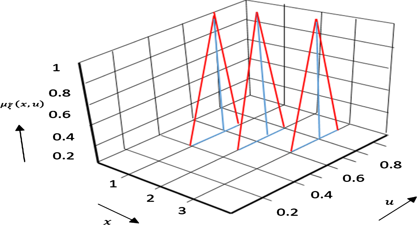
Type-2 fuzzy variable ${\tilde{γ}}_{p}^{intra}$ .

To solve the example, in the first stage, we apply a CV reduction method to convert the type-2 fuzzy variables to corresponding type-1 fuzzy variables. In the second stage, we apply a centroid method to reduction type-1 fuzzy variables to crisp values. The crisp values of technological coefficients are obtained as $γ_{p}^{intra} = (2.07, 3.07),$ $γ_{p}^{intra} = (10.03, 15.03),$ λ_t = (48.91, 58.91) and φ_m = (2874.3, 3874.3).

For example, we consider the following discrete RFV for ${\tilde{γ}}_{p}^{intra}$ : ${\tilde{γ}}_{p}^{intra} = {\begin{matrix} 1 & \tilde{μ} {\tilde{γ}}_{p}^{intra} = (0.4, 0.6, 0.7) \\ 2 & \tilde{μ} {\tilde{γ}}_{p}^{intra} = (0.5, 0.7, 0.8) \\ 3 & \tilde{μ} {\tilde{γ}}_{p}^{intra} = (0.6, 0.8, 0.9) \end{matrix}$

Then, we have: $\begin{matrix} {CV}^{*} [1] = 0.64, {CV}_{*} [1] = 0.5, CV [1] = 0.57 \\ {CV}^{*} [2] = 0.73, {CV}_{*} [2] = 0.58, CV [2] = 0.64 \\ {CV}^{*} [3] = 0.81, {CV}_{*} [3] = 0.67, CV [3] = 0.71 \end{matrix}$

Type-1 fuzzy variables are obtained by using the optimistic, pessimistic and CV reduction methods to ${\tilde{γ}}_{p}^{intra}$ (i.e., intra cell movement cost for part type 1), respectively as follows: $\begin{matrix} (\begin{matrix} 1 & 2 & 3 \\ 0.64 & 0.73 & 0.81 \end{matrix}) (\begin{matrix} 1 & 2 & 3 \\ 0.5 & 0.58 & 0.67 \end{matrix}) \\ (\begin{matrix} 1 & 2 & 3 \\ 0.57 & 0.64 & 0.71 \end{matrix}) \end{matrix}$

The CV reduction method uses the credibility measures (i.e., average of necessity and possibility measures) while pessimistic CV and optimistic CV reduction methods are developed by using necessity and possibility measures, respectively. We take the defuzzified value derived by using the CV reduction method [18]. Applying the centroid method to these type-1 fuzzy variables, we obtain the corresponding reduced crisp value. $γ_{p}^{intra} = 2.07$ .

By considering the data provided in Tables 1 to 3, and crisp coefficients that are the results of the defuzzification process, the detailed optimal solution of the proposed model is presented in Tables 4 and 5.

Table 4

Objective functions and components for the developed type-2 fuzzy programming example

Total	Total Processing cost	Inter-cell Material cost	Intra-cell materialcost	Total machine constant cost	Tooling cost
26533.89	6000	0	82.45	20245.8	205.64

Table 5

Optimal selection of cells, locations, machines, operations, tools and operators for the developed type-2 fuzzy programming example

Cells	Locations	Machines	Tools	Operators	p ₁		p ₂		Number of tool	Number of Machines	Number of operators
					j ₁	j ₂	j ₁	j ₂
C ₃	L ₃	M ₁	T ₁	W ₁		10			1	3	1
		–	T ₂		9				1	–	–
C ₁	L ₁	M ₂	T ₁	W ₂			10	12	2	3	1
		–	T ₂						–	–	–
C ₂	L ₂	–	–	–	–	–	–	–	–	–	–

5 Solution algorithms

The notable advantage of a meta-heuristic algorithm is its ability in solving NP-hard problems. A number of authors, (e.g., [20, 52]) proposed meta-heuristics to solve large-sized problems considering their computational time. Due to the NP-hardness of the proposed model, it is necessary to develop a meta-heuristic approach to solve the proposed model for large-sized problems. To solve the problem, this paper presents a particle swarm optimization, due to there is no benchmark available to validate the results, two meta-heuristic algorithms as differential evolution (DE) and Firefly algorithm (FA) are presented too. In addition, in order to obtain better solutions, the Taguchi method is used to tune the parameters of three algorithms. The details of the algorithms are given in the next subsections.

5.1 Particle swarm optimization

The particle swarm optimization (PSO) algorithm is a population-based stochastic optimization algorithm that was established by Kennedy and Eberhart [14]. It is composed of a population (i.e., swarm) of candidate solutions, called particles. These particles are in motion inward the search-space with a denoted velocity in search of an optimal solution. Each particle preserves a memory, which helps it in keeping the path of its previous best position. The positions of the particles are recognized as personal best and global best [32]. The main iterative process to determine the solution is performed by: $x_{i}^{k + 1} = x_{i}^{k} + v_{i}^{k + 1}$ (50) $\begin{matrix} v_{i}^{k + 1} & = & {wv}_{i}^{k} + C_{1} {rand}_{1} ({PBest}_{i} - x_{i}^{k}) \\ + C_{2} {rand}_{2} (P_{gi} - x_{i}^{k}) \end{matrix}$ (51)

Equation (48) calculates the movement for the ith particle in the kth iteration, where $v_{i}^{k}, x_{i}^{k}$ is the velocity and the current position of the ith particle in the kth iteration, respectively. Equation (51) calculates the updated velocity vector of the ith particle in the kth iteration, PBest_i is the best position of the ith particle, w is the inertia factor that controls the magnitude of the old velocity, C₁ and C₂ are acceleration constants (i.e., cognitive and social) and based on the kind of search, local or global P_gi called lBest and gBest [32].

5.2 Differential evolution algorithm

The differential evolution (DE) algorithm is a very recent evolutionary techniques for optimizing continuous nonlinear functions and developed by Noktehdan et al. [31] and Storn and Price [44]. The main steps of the DE algorithm are defined as follows. First, a random generation of a population is formed and evaluation of the objective function is performed. For each individual solution in the current population, creation of a mutated solution ${\hat{x}}_{i}$ (52) is as foolows:

$\hat{x_{i}} = x_{r 1} + F (x_{r 3} - x_{r 2})$ (53)

where F is a scalar (F ∈ [0, 1]), and x_r1, x_r3, x_r2 are randomly chosen individuals in the current population i ( $\hat{x_{i}} \neq x_{r 1} \neq x_{r 3} \neq x_{r 2}$ ). The crossover operation is used to construction a trial vector by shuffling the information contained in the mutated vector and the current solution. $y_{i}^{j} = {\begin{matrix} {\hat{x}}_{i}^{j} & R_{j} \leq CR \\ x_{i}^{j} & R_{j} > CR \end{matrix}$ (54)

CR is the crossover rate ∈[0, 1] which has to be determined by the user, and R_j is a random real number ∈[0, 1] and j is j.th parameter. Each trial vector ( $\vec{y_{i}}$ ) is compared with its parent ( $\vec{x_{i}}$ ) and the better one is remained in the population in the selection step [38].

5.3 Firefly algorithm

Firefly algorithm (FA) is a nature-inspired meta-heuristic global optimization method, which is based on the flashing light of fireflies and developed by Yang [55]. A females firefly attracts males fireflies equivalent to the brightness and the distance. Females Firefly prefer brighter male flashes also the flash intensity varies with the distance from the source. A less brighter firefly moves towards to the adjacent brighter one [38, 41]. The main steps of the FA algorithm are defined as follows: First, the random firefly positions (solutions) with the limits of problem variables and control parameters of the FA algorithm is initialized. The brightness of a firefly is determined by evaluating the landscape of the objective function. The variation of attractiveness of a firefly (β) determined with the distance r by: $β = β_{0} e^{- γ r^{2}}$ (55)

where β₀ is the attractiveness at r = 0.

The Cartesian distance (r) is used for shown distance between two fireflies. γ is the absorption coefficient of light and effects on the speed of convergence. The movement of a less attractive firefly (ith) towards a most attractive firefly (jth) is defined by Equation 53: $x_{i}^{t + 1} = x_{i}^{t} + β_{0} e^{- γ r_{ij}^{2}} (x_{j}^{t} - x_{i}^{t}) + α_{t} ɛ_{i}^{t}$ (56) where, ɛ_i is a random number and α is randomization constraint [37, 40].

6 Computational results

In order to verify and validate the proposed model and evaluate the performance of three meta-heuristic algorithms on the CMS design, a range of random numerical examples are generated. for solve the presented model MATLAB (R2013b) software is used to code the algorithms on a laptop including five Intel (R) core (TM) i5-3230 CPU @ 2.60 GHz and 6 GB RAM. The Taguchi method is performed in MINITAB software version 16.2.2 to tune the parameters and analysis of the data.

6.1 Generating random data

10 random examples are constructed in different sizes by uniform distributed random points for some of the parameters provided. Four effective factors on the size of each problem is given.

The number of operations (J)

The number of parts (P)

The number of machines (M)

The number of workers (W)

The attributes of 10 designed test examples are shown in Tables 6. Also, Table 7 shows the details of the model input parameters required for 10 problem instances.

Table 6
The attribute of test examples

Problem No 1 2 3 4 5 6 7 8 9 10

J 2 3 3 4 4 5 5 6 6 7

P 3 3 4 4 5 6 7 6 7 8

M 3 3 4 4 4 5 5 4 4 5

W 3 3 4 4 4 5 5 4 4 5

Problem No	1	2	3	4	5	6	7	8	9	10
J	2	3	3	4	4	5	5	6	6	7
P	3	3	4	4	5	6	7	6	7	8
M	3	3	4	4	4	5	5	4	4	5
W	3	3	4	4	4	5	5	4	4	5

Table 7

Information relating to random production of problems test

Parameter	Amount	Parameter	Amount
t _jpmtw	0.03	$t_{jpmtw}^{'}$	0.02
$γ_{p}^{inter}$	U (10.03–15.03)	$t_{jpmtw}^{''}$	0
$γ_{p}^{intra}$	U (2.07–3.07)	K _jpmtw	U (9–16)
D _p	U (100–200)	φ _m	U (2874.3–3874.3)
T _m	45	Q _t	3
T _w	45	TQ _m	7
β _m	U (2–3)	λ _t	U (48.91–58.91)
α _w	U (1–2)	$B_{p}^{inter}$	U (12–15)
$B_{p}^{intra}$	U (2–5)	TL _t	1

6.2 Tuning parameters

In this section the Taguchi method is employed to tune the parameters of the PSO, FA and DE Algorithms, because the values of meta-heuristic algorithms parameters affected on quality of the solution. Taguchi method is a fractional factorial experiment proposed by Taguchi useable as an efficient alternative for full factorial experiments [40]. Taguchi procedure uses orthogonal array for design of experiences and then applied a procedure to reduction of the variation and control of N [27]. There are different types of the quality characteristic the S/N, but in this study, the “smaller is better” type of response has been used (since the goal is to minimize S/N), where S/N is given as $S / - N = - 10 \times Log (\frac{S (y^{2})}{n})$ (57)

Where, n and Y are the number of orthogonal arrays the response, respectively. To execute the Taguchi procedure, we use the L⁹ design, in which the values and levels of PSO, FA and DE algorithm parameters are given in Table 8. These values are obtained after multiple tests on the current examples of the classes using the frequent runs of the algorithms.

Table 8

PSO, FA and DE parameters and levels

	Algorithm Parameters	LEVEL (1)	LEVEL (2)	LEVEL (3)
PSO	NOP (A)	30	40	50
	C₁ (B)	1.5	2	2.5
	C₂ (B)	1.5	2	2.5
	NOG (D)	100	150	200
FA	NOG (A)	20	50	100
	NOP (B)	15	30	40
	ALFA (C)	0.2	0.5	0.9
DE	NOP (A)	20	30	50
	NOG (B)	30	50	100
	P_c (C)	0.1	0.5	0.9

6.3 Analysis of results

In order to compare the results obtained from three algorithms and find the best methodology for solving the proposed CMS design with type-2 fuzzy variables, each other of the 10 generated examples, solved by MATLAB (R2013b) soft wares on a laptopincluding five Intel (R) core (TM) i5-3230 CPU @ 2.60 GHz and 6 GB RAM. Tables 9 to 11 contains the input parameter and the objective values of three algorithms for each one of the examples. In these Tables, the optimal values of the algorithm parameters are obtained with L₉ design using the Taguchi method.

Table 9
Input parameters and the objective function of the PSO algorithm for the generated problems

Problem No. PSO

NOP C1 C2 NOG OBJ

1 40 2.5 2.5 150 18729

2 40 2.5 2.5 150 36527

3 40 1.5 2 150 51355

4 40 1.5 2.5 200 89909

5 50 1.5 2 150 76227

6 50 2.5 2.5 150 155380

7 40 1.5 2 200 204020

8 50 1.5 1.5 200 166830

9 40 1.5 2 200 162970

10 30 1.5 1.5 200 227730

MEAN – – – – 118968

St. Dev – – – – 73562

Problem No.	PSO
1	40	2.5	2.5	150	18729
2	40	2.5	2.5	150	36527
3	40	1.5	2	150	51355
4	40	1.5	2.5	200	89909
5	50	1.5	2	150	76227
6	50	2.5	2.5	150	155380
7	40	1.5	2	200	204020
8	50	1.5	1.5	200	166830
9	40	1.5	2	200	162970
10	30	1.5	1.5	200	227730
MEAN	–	–	–	–	118968
St. Dev	–	–	–	–	73562

Table 10

Input parameters and the objective function of the FA algorithm for the generated problems

Problem No.	FA
	NOG	NOP	ALFA	OBJ
1	100	40	0.9	29633
2	100	40	0.2	53518
3	20	40	0.9	75455
4	50	30	0.2	140210
5	50	40	0.9	118110
6	20	30	0.2	205570
7	50	40	0.9	235150
8	20	40	0.9	188630
9	20	40	0.5	214460
10	50	30	0.2	317320
MEAN	–	–	–	157806
St. Dev	–	–	–	90578

Table 11

Input parameters and the objective function of the DE algorithm for the generated problems

Problem No.	DE
	NOP	NOG	PC	OBJ
1	50	100	0.1	42102
2	50	100	0.1	44352
3	50	100	0.1	85693
4	30	100	0.1	96351
5	30	50	0.9	96130
6	30	100	0.9	193910
7	50	100	0.9	249700
8	50	100	0.9	190150
9	50	100	0.1	189760
10	30	100	0.5	231620
MEAN	–	–	–	141977
St. Dev	–	–	–	77315

In addition to, according to Fig. 6, it look like that PSO has a better performance than FA and DE in objective function in all problems. The one-way analysis of variance (ANOVA) is used to compare the performances of the PSO, FA and DE algorithm statistically.

Fig.6

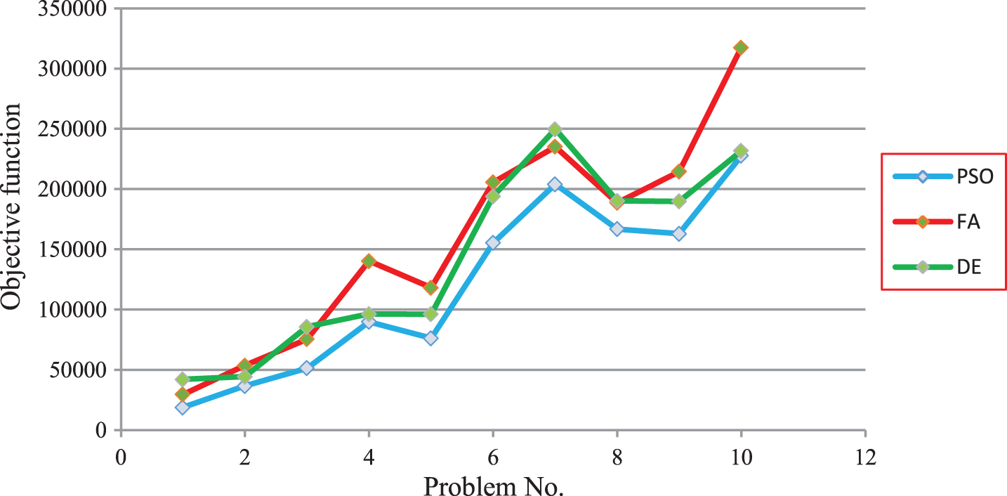
Trend of objective function values of the generated problems for the proposed algorithms.

This process is performed in MINITAB software version 16.2.2. The ANOVA output shown in Table 12 indicates that at a confidence level of 95% the two algorithms do not have significant differences in the Mean objective function. Performances of three algorithms can also be observed in Fig. 7.

Fig.7

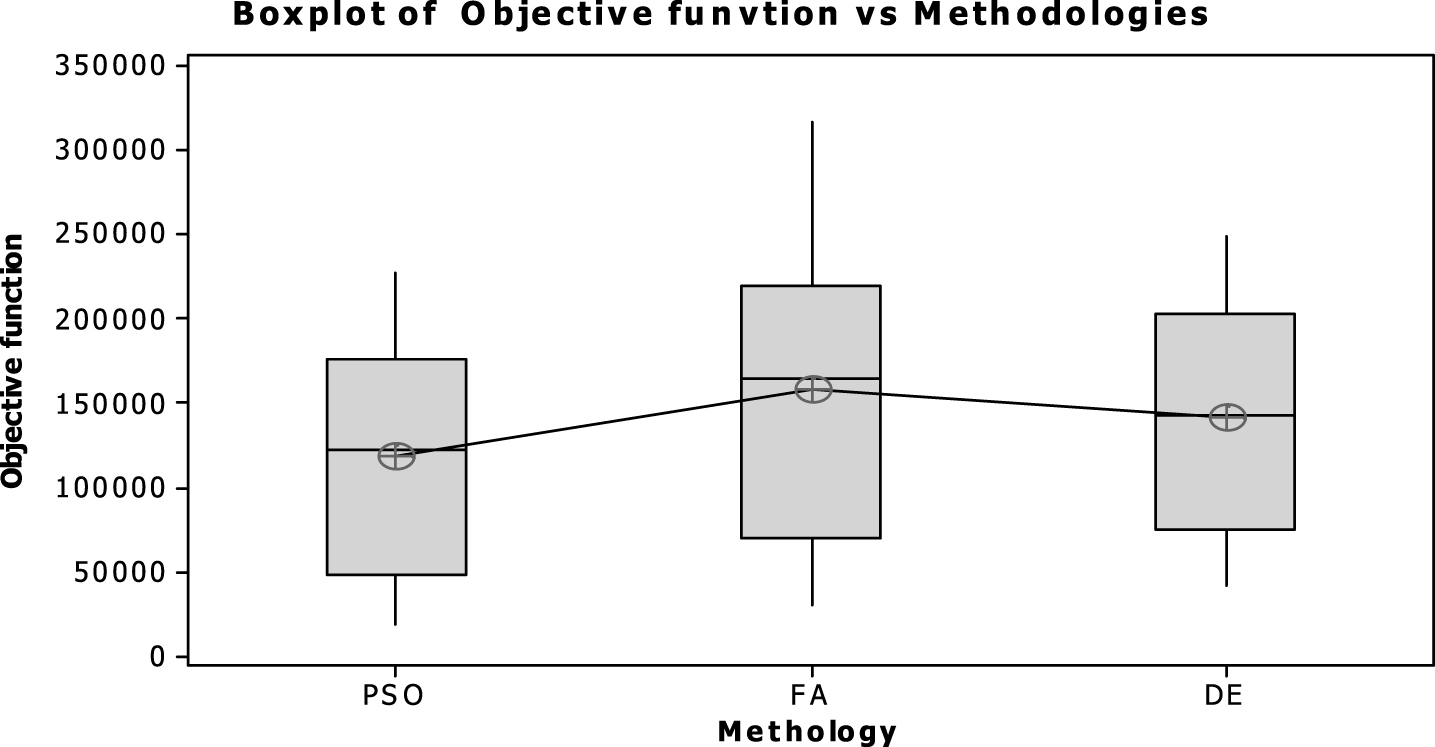
Boxplot of the objective function values.

Table 12

Analysis of variance results to compare the algorithms in terms of mean objective function value

Source	DF	SS	MS	F	P-value
Methods	2	7627840229	3813920114	0.58	0.565
Error	27	1.76341E+11	6531130466
Total	29	1.83968E+11

7 Conclusions

In this research, an integrating model for cell formation, inter cell-layout, resource assignment consist of tool assignment and operator assignment problems was investigated for the cellular manufacturing system design with the total expected cost criteria. In our presented model, processing cost, inter and intra-cell material handling costs, machines constant cost and tooling cost were minimized. The distinguished benefits of the mathematical model were as follows: cell formation by more material flow to the shortest distances and operator assignment by the total expected cost criteria with the desirable costs that defined by Fuzzy type-2. By utilizing a number of auxiliary variables, the presented model was linearized. We solved a small-sized numerical example with Type-2 fuzzy variables by a branch-and-bound (B&B) method using Lingo 9.0 software.

To solve the proposed CMS model, a PSO algorithm was employed, in which DE and FA were used to validate the outputs of the presented algorithm. The Taguchi method was used to tune of the PSO, DE and FA algorithms. One of the notable advantage of this research to solve 10 generated random large-sized problems was used the optimal levels of the algorithms parameters by the Taguchi method for each problem. The results of the algorithms showed that the PSO algorithm had a better performance than the DE and FA in terms of the objective function on 10 generated random problems. The one-way analysis of variance (ANOVA) was used to compare the performances of the PSO, DE and FA algorithms statistically. Also, the tendency displayed that PSO had better performances in comparison with DE and FA in most problems, in which a statistical significant difference was not found. This shows that the valid results were derived using PSO. Finally, some recommendations for further research are as follows:

Used the other meta-heuristic algorithms.

Extending the model in other fuzzy type – 2 parameters.

Considering the proposed model in multi period planning horizon.

As a direction for future research, it would be interesting to consider the Response surface methodology to set the algorithms parameters.

References

Al-Ahmari

and Alharbi

, Design of cellular manufacturing systems with labor and tools consideration, Proceeding of the International Conference on Computers and Industrial Engineering, Troyes, France, 2009, pp. 678–683.

Aryanezhad

M.B.

, Deljoo

, Mirzapour

S.M.J.

, Al-e-Hashem , Dynamic cell formation and the worker assignment problem: A new model, The International Journal of Advanced Manufacturing Technology 41 (2008), 329–342.

Azadeh

, Nazari-Shirkouhi

, Hatami-Shirkouhi

and Ansarinejad

, A unique fuzzy multi-criteria decision making: Computer simulation approach for productive operators’ assignment in cellular manufacturing systems with uncertainty and vagueness, The International Journal of Advanced Manufacturing Technology 56 (2011), 329–343.

Bagheri

and Bashiri

, A new mathematical model towards the integration of cell formation with operator assignment and inter-cell layout problems in a dynamic environment, Applied Mathematical Modelling 38 (2014), 1237–1254.

Balakrishnan

and Cheng

C.H.

, Dynamic cellular manufacturing under multiperiod planning horizons, Journal of Manufacturing Technology Management 16 (2005), 516–530.

Chen

and Cao

, Coordinating production planning in cellular manufacturing environment using Tabu search, Computers and Industrial Engineering 46 (2004), 571–588.

Deljoo

, Mirzapour Al-e-hashem

S.M.J.

, Deljoo

and Aryanezhad

M.B.

, Using genetic algorithm to solve dynamic cell formation problem, Applied Mathematical Modelling 34 (2010), 1078–1092.

Dimopoulos

and Zalzala

, Recent developments in evolutionary computing for manufacturing optimization: Problems, solutions and comparisons, IEEE Transactions on Evolutionary Computation 68 (2000), 93–113.

Fazlollahtabar

, Mahdavi-Amiri

and Muhammadzadeh

, A genetic optimization algorithm for nonlinear stochastic programs in an automated manufacturing system, Journal of Intelligent & Fuzzy Systems 28 (2015), 1461–1475.

10.

García

J.C.F.

, Solving fuzzy linear programming problems with Interval Type-2 RHS, IEEE International Conference on Systems, Man and Cybernetics, San Antonio, USA, 2009, pp. 262–267.

11.

Hamedi

, Esmaeilian

G.R.

, Ismail

and Ariffin

M.K.A.

, Capability-based virtual cellular manufacturing systems formation in dual-resource constrained settings using Tabu Search, Computers and Industrial Engineering 62 (2012), 953–971.

12.

Heragu

S.S.

and Kakuturi

S.R.

, Grouping and placement of machine cells, IIE Transactions 29 (1997), 561–571.

13.

Jain

A.K.

, Kasilingam

R.G.

and Bhole

S.D.

, Joint consideration of cell formation and tool provisioning problems in flexible manufacturing systems, Computers and Industrial Engineering 20 (1991), 271–277.

14.

Kennedy

and Eberhart

, Particle swarm optimization, Paper presented at the Neural Networks, Proceedings of the IEEE International Conference, Perth, WA, 1995, pp. 1942–1948.

15.

Kia

, Baboli

, Javadian

, Tavakkoli-Moghaddam

, Kazemi

and Khorrami

, Solving a group layout design model of a dynamic cellular manufacturing system with alternative process routings, lot splitting and flexible reconfiguration by simulated annealing, Computers and Operations Research 39 (2012), 2642–2658.

16.

Kia

, Khaksar-Haghani

, Javadian

and Tavakkoli-Moghaddam

, Solving a multi-floor layout design model of a dynamic cellular manufacturing system by an efficient genetic algorithm, Journal of Manufacturing Systems 33 (2014), 218–232.

17.

Kia

, Tavakkoli-Moghaddam

, Javadian

, Baboli

and Kazemi

, A group layout design model of a dynamic cellular manufacturing system, Proceeding of the IEEE 3rd International Conference on Communication Software and Networks, Xi’an, China, (2011), pp. 745–749.

18.

Kundu

, Kar

and Maiti

, Fixed charge transportation problem with type-2 fuzzy variables, Information Sciences 255 (2014), 170–186.

19.

Logendran

, Ramakrjshna

and Sriskandarajah

, Tabu search-based heuristics for cellular manufacturing systems in the presence of alternative process plans, International Journal of Production Research 32 (1994), 273–297.

20.

Mahdavi

, Paydar

M.M.

, Solimanpur

and Heidarzade

, Genetic algorithm approach for solving a cell formation problem in cellular manufacturing, Expert Systems with Applications 36 (2009), 6598–6604.

21.

Mahdavi

, Aalaei

, Paydar

M.M.

and Solimanpur

, Designing a mathematical model for dynamic cellular manufacturing systems considering production planning and worker assignment, Computers and Mathematics with Applications 60 (2010), 1014–1025.

22.

Mahdavi

, Teymourian

, Tahami Baher

and Kayvanfar

, An integrated model for solving cell formation and cell layout problem simultaneously considering new situations, Journal of Manufacturing Systems 32 (2013), 655–663.

23.

Mahdavi

, Bootaki

and Paydar

M.M.

, Manufacturing cell configuration considering worker interest concept applying a bi-objective programming approach, International Journal of Industrial Engineering and Production Research 25 (2014), 41–53.

24.

Majazi Dalfard

, New mathematical model for problem of dynamic cell formation based on number and average length of intra and intercellular movements, Applied Mathematical Modelling 37 (2013), 1884–1896.

25.

Mehdizadeh

and Rahimi

, An integrated mathematical model for solving dynamic cell formation problem considering operator assignment and inter/intra cell layouts, Applied Soft Computing 42 (2016), 325–341.

26.

Min

and Shin

, Simultaneous formation of machine and human cells in group technology: A multiple objective approach, International Journal of Production Research 31 (1993), 2307–2318.

27.

Mousavi

S.M.

, Hajipour

, Niaki

S.T.A.

and Aalikar

, A multi-product multi-period inventory control problem under inflation and discount: A parameter-tuned particle swarm optimization algorithm, The International Journal of Advanced Manufacturing Technology 70 (2014), 1739–1756.

28.

Mungwattana

Design of cellular manufacturing systems for dynamic and uncertain production requirement with presence of routing flexibility, Ph.D. Thesis, Blacksburg State University Virginia, 2000.

29.

Niebel

B.W.

, Motion and time study, Homewood, Irwin, USA, 1982.

30.

Norman

B.A.

, Tharmmaphornphilas

, Needy

K.L.

, Bidanda

and Warner

R.C.

, Worker assignment in cellular manufacturing considering technical and human skills, International Journal of Production Research 40 (2002), 1479–1492.

31.

Noktehdan

, Karimi

and Husseinzadeh Kashan

, A differential evolution algorithm for the manufacturing cell formation problem using group based operators, Expert Systems with Applications 37 (2010), 4822–4829.

32.

Pant

, Thangaraj

and Abraham

, Particle swarm optimization: Performance tuning and empirical analysis foundations of computational intelligence, Global Optimization 3 (2009), 101–128.

33.

Qin

, Liu

Y.K.

and Liu

Z.Q.

, Methods of critical value reduction for type-2 fuzzy variables and their applications, Journal of Computational and Applied Mathematics 235 (2011), 1454–1481.

34.

Rafiei

and Ghodsi

, A bi-objective mathematical model toward dynamic cell formation considering labor utilization, Applied Mathematical Modelling 37 (2013), 2308–2316.

35.

Safaei

, Saidi-Mehrabad

and Jabal-Ameli

M.S.

, A hybrid simulated annealing for solving an extended model of dynamic cellular manufacturing system, European Journal of Operational Research 185 (2008), 563–592.

36.

Safaei

, Saidi-Mehrabad

, Tavakkoli-Moghaddam

and Sassani

, A fuzzy programming approach for a cell formation problem with dynamic and uncertain conditions, Fuzzy Sets and Systems 159 (2008), 215–236.

37.

Safaei

and Tavakkoli-Moghaddam

, Integrated multi-period cell formation and subcontracting production planning in dynamic cellular manufacturing systems, International Journal of Production Economics 120 (2009), 301–314.

38.

Sahin

and Akay

, Comparisons of metaheuristic algorithms and fitness functions on software test data generation, Applied Soft Computing 49 (2016), 1202–1214.

39.

Selim

H.M.

, Askin

R.G.

and Vakharia

A.J.

, Cell formation in group technology: Review, evaluation and directions for future research, Computers and Industrial Engineering 34 (1998), 3–20.

40.

Shavandi

, Mahlooji

and Ekram Nosratian

, A constrained multi-product pricing and inventory control problem, Applied Soft Computing 12 (2012), 2454–2461.

41.

Shukla

and Singh

, Selection of parameters for advanced machining processes using firefly algorithm, Engineering Science and Technology, an International Journal (2016).

42.

Slomp

, Chowdary

B.V.

and Suresh

N.C.

, Design of virtual manufacturing cells: A mathematical programming approach, Robotics and Computer-Integrated Manufacturing 21 (2005), 273–288.

43.

Solimanpur

, Vrat

and Shankar

, Ant colony optimization algorithm to the inter-cell layout problem in cellular manufacturing, European Journal of Operational Research 157 (2004), 592–606.

44.

Storn

and Price

, Differential evolution - a simple and efficient heuristic for global optimization over continuous spaces, Journal of Global Optimization 11 (1997), 341–359.

45.

Süer

G.A.

and Bera

I.S.

, Optimal operator assignment and cell loading when lot-splitting is allowed, Computers and Industrial Engineering 35 (1998), 431–434.

46.

Sugeno

, Theory of fuzzy integrals and its applications, Ph.D. Thesis, Tokyo Institute of Technology, 1974.

47.

Sugeno

, An introductory survey of fuzzy control, Information Sciences 36 (1985), 59–83.

48.

Suresh

N.C.

, Slomp

and Kaparthi

, Sequence-dependent clustering of parts and machines: A Fuzzy ART neural network approach, International Journal of Production Research 37 (1999), 2793–2816.

49.

Tavakkoli-Moghaddam

, Aryanezhad

M.B.

, Safaei

and Azaron

, Solving a dynamic cell formation problem using metaheuristics, Applied Mathematics and Computation 170 (2005), 761–780.

50.

Tavakkoli-Moghaddam

, Aryanezhad

M.B.

, Safaei

, Vasei

and Azaron

, A new approach for the cellular manufacturing problem in fuzzy dynamic conditions by a genetic algorithm, Journal of Intelligent & Fuzzy Systems 18 (2007), 363–376.

51.

Tavakkoli-Moghaddam

, Javadi

, Jolai

and Mirgorbani

S.M.

, An efficient algorithm to inter and intra-cell layout problems in cellular manufacturing systems with stochastic demands, IJE Transactions A: Basics 19 (2006), 67–78.

52.

Tavakkoli-Moghaddam

, Heydar

and Mousavi

S.M.

, A hybrid genetic algorithm for a bi-objective scheduling problem in a flexible manufacturing cell, IJE Transactions A: Basics 23 (2010), 235–252.

53.

Vakharia

A.J.

and Chang

Y.L.

, Cell formation in group technology: A combinatorial search approach, International Journal of Production Research 35 (1997), 2025–2044.

54.

Wemmerlöv

and Hyer

N.L.

, Procedures for the part family/machine group identification problem in cellular manufacturing, Journal of Operations Management 6 (1986), 125–147.

55.

Yang

X.S.

, Nature-Inspired Metaheuristic Algorithm, Luniver Press, United Kingdom, 2008.

56.

Zadeh

L.A.

, The concept of a linguistic variable and its application to approximate reasoning-II, Information Sciences 8 (1975), 301–357.

An integrated cellular manufacturing system with type-2 fuzzy variables: Three tuned meta-heuristic algorithms

Abstract

Keywords

1 Introduction

2 Problem description

2.1 Assumptions

2.2 Notations

2.2.1 Input parameters

2.2.2 Decision variables

2.2.3 Auxiliary variables

2.3 Mathematical model

3.1 Fundamental concepts and definitions

3.3 Critical values (CV) for RFVs

5.1 Particle swarm optimization

6.1 Generating random data

Table 6 The attribute of test examples Problem No 1 2 3 4 5 6 7 8 9 10 J 2 3 3 4 4 5 5 6 6 7 P 3 3 4 4 5 6 7 6 7 8 M 3 3 4 4 4 5 5 4 4 5 W 3 3 4 4 4 5 5 4 4 5

References

Table 6
The attribute of test examples

Problem No 1 2 3 4 5 6 7 8 9 10

J 2 3 3 4 4 5 5 6 6 7

P 3 3 4 4 5 6 7 6 7 8

M 3 3 4 4 4 5 5 4 4 5

W 3 3 4 4 4 5 5 4 4 5