An empirical assestment of fuzzy Black and Scholes pricing option model in Spanish stock option market

Abstract

The main objective of this paper is assessing the empirical performance of fuzzy extension to Black-Scholes option pricing formula (FBS). Concretely we evaluate the goodness of the FBS predictions for traded prices of options on the Spanish stock index IBEX35 during March 2017. We firstly propose a procedure to fit, from real data, the fuzzy parameters to implement FBS in stock options: price of the subjacent asset, free discount rate and stock volatility. Subsequently we evaluate the capability of FBS to include actual traded prices and whether this capability depends on option moneyness and expiration date. We find that FBS fits quite well actual traded prices. However, generally most representative market prices (closing and medium) are not better fitted than those more extreme (minimum and maximum). We have also check that the goodness of the FBS predictions often depends on the moneyness grade and the expiration date of options.

Keywords

Fuzzy numbers fuzzy regression expected interval of fuzzy numbers finance option pricing Black-Scholes formula

1 Introduction

In economic and financial problems, an important piece of information is often given by means of imprecise and/or vague data. In this case Fuzzy Set Theory (FST) is a suitable modeling instrument. This reason explains why, despite stochastic analysis is at the core of option pricing methods; their extension to the use of fuzzy parameters has become an active research field. Some works in this way are [7, 43] for real options and [3 , 44] for financial options of European or American style. Likewise [36, 37] develop fuzzy methodologies to price less common option styles like compounded options or binary options. These papers usually develop deeply several aspects of fuzzy extension to the model by Black and Scholes [1], (FBS). Likewise, other options pricing models have been extended to fuzziness in parameters. Whereas [28] propose a fuzzy option pricing method where the subjacent asset follows a geometric Brownian motion with Poisson jumps, [12] extends the model with stochastic volatility by Heston [16] to the case where some parameters are fuzzy numbers. Zhang et al. [42] extend the double exponential jump diffusion model to price European options to fuzzy environments. Papers [28, 29] develop a fuzzy option pricing to the case where the subjacent asset follows a Levy process. In any case, for a wide review on this matter see [27].

This study is motivated by the scarceness of papers about the empirical performance of fuzzy option models. In contrast, there is a great deal of literature on theoretical fuzzy option pricing as we exposed above. Concretely, we analyze two empirical aspects about fuzzy extension of Black-Scholes formula. We firstly propose a procedure to quantify parameters from empirical data to implement FBS by means of Triangular Fuzzy Numbers. Subsequently we evaluate the suitability of FBS to predict actual traded option prices. The empirical application is developed with a sample of closing, maximum, mean and minimum prices of calls and puts for IBEX35 traded in the Spanish Derivative Market (MEFFSA) within the Wednesdays of March 2017. We test the closeness of FBS to actual prices from two perspectives. We initially evaluate the membership level of observed prices into the fuzzy estimates that come from FBS. Alternatively we analyze the frequency in which the expected interval of FBS contains actual prices. In both cases we also study if moneyness and maturity of options have influence in the performance of FBS to fit real data. We find that FBS fits quite well actual traded option prices and that there is not a substantial difference between call and put options on this matter. However, generally representative market prices (closing and medium) are not better fitted than minimum and maximum prices. We have also checked that the moneyness grade and the expiration of the option influence the goodness of FBS predictions.

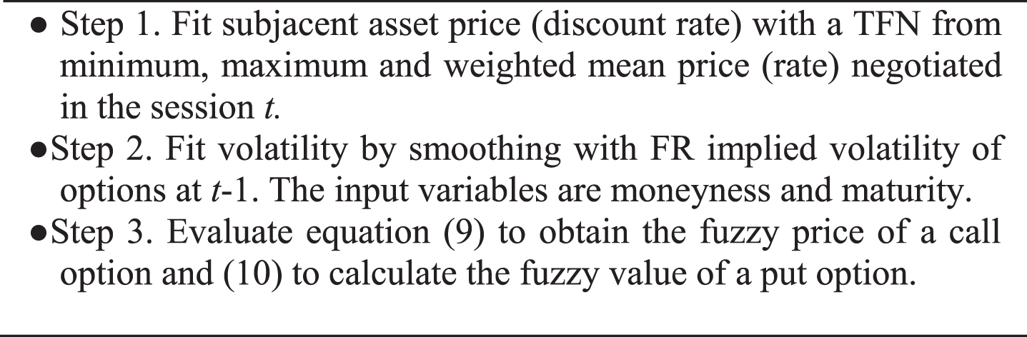
We structure the rest of the paper as follows. In section 2 we describe the notation and instruments of FST used in this paper. We then present the fuzzy extension to the formula in [1] in [38, 39] and propose a way to obtain fuzzy estimates for subjacent asset price, free discount rate and volatility from empirical data. Whereas the fuzzy estimates of stock price and free discount rate comes straightforward from empirical data, to obtain the volatility we smooth options past implied volatilities using a fuzzy regression model, similarly to [26]. Subsequently we assess the goodness of FBS to fit traded prices. Finally we outline the principal conclusions of our paper.

2 Functions of fuzzy variables and fuzzy regression

A fuzzy set $\tilde{A}$ can be defined as $\tilde{A} = {(x, μ_{\tilde{A}} (x)) | x \in X}$ , where $μ_{\tilde{A}}$ is the membership function and is a mapping $μ_{\tilde{A}} : X \to [0, 1]$ . Alternatively, a fuzzy set can be represented by its α-cuts, A_α, where $A_{α} = {x \in X | μ_{\tilde{A}} (x) \geq}, \forall \in (0, 1]$ .

A Fuzzy Number (FN) is a fuzzy subset $\tilde{A}$ defined over the set of real numbers. It is normal, i.e. $\max_{x \in X} μ_{\tilde{A}} (x) = 1$ , and convex, that is, its α-cuts are closed and bounded intervals. So, they can be represented as $A_{α} = [\underline{A} (α), \bar{A} (α)]$ , where $\underline{A} (α) (\bar{A} (α))$ are continuously increasing (decreasing) functions of the membership level (ML) αɛ [0, 1]. Triangular Fuzzy Numbers (TFNs) are used intensively in practical applications of FST. A TFN can be denoted as $\tilde{A} = (a, l_{a}, u_{a})$ where the value a is the core whereas l_a and u_a are the lower and upper spread of that FN. The α-cut representation of a TFN is: $A_{α} = [a - l_{a} (1 - α), a + r_{a} (1 - α)]$ (1)

The expected interval (EI) of a FN is commonly used in fuzzy literature to estimate a representative real valued interval of a FN. It was developed, among others, by Heilpern in [15]. If we name the EI of $\tilde{A}$ , $EI (\tilde{A}),$ analytically: $EI (\tilde{A}) = [\int_{0}^{1} \underline{A} (α) d α, \int_{0}^{1} \bar{A} (α) d α]$ (2)

Let f (·) be a continuous real valued function of n-real variables x_j, j = 1, 2, …, n, and let ${\tilde{A}}_{1}, {\tilde{A}}_{2}, \dots, {\tilde{A}}_{n}$ be n FNs that quantify these variables. Although often the membership function of $\tilde{B} = f ({\tilde{A}}_{1}, {\tilde{A}}_{2}, \dots, {\tilde{A}}_{n})$ , can be obtained it is usually possible to obtain a closed expression for its α-cuts, B_α. If f (·) is increasing with respect to the first m variables, m ≤ n, and decreases in the last n - m variables, from [4]:

$\begin{array}{l} B_{α} = [\underline{B} (α), \bar{B} (α)] \\ = [f (\underline{A_{1}} (α), \underline{A_{2}} (α), \dots, \underline{A_{m}} (α), {\bar{A}}_{m + 1} (α), {\bar{A}}_{m + 2} (α), \dots {\bar{A}}_{n} (α)) \\ f ({\bar{A}}_{1} (α), {\bar{A}}_{2} (α), \dots, {\bar{A}}_{m} (α), \underline{A_{m + 1}} (α), \underline{A_{m + 2}} (α), \dots \underline{A_{n}} (α))] \end{array}$ (3)

The fuzzy regression (FR) model used in this paper is developed in [17]. This method mixes least squares (LS) regression and the FR method in [35] but also allow a non-symmetrical structure for the coefficients. In our concrete option pricing context, [26] evaluate how several FR methods (including [17]) fit the volatility smile of options.

Like any regression technique, the objective of a FR method is to determine a functional relationship between a dependent variable (output) and a set of independent ones (inputs). Let us suppose that for the j-th observation of the sample, j = 0, 1, …, n, the pair of the dependent variable (that may be a FN) and the independent variables (that we suppose crisp) is $({\tilde{y}}_{j}, x_{j})_{j = 1, 2, \dots, n}$ where x_j = (x_1,j, x_2,j, …, x_m,j), ${\tilde{y}}_{j} = (y_{j}, l_{y_{j}}, r_{y_{j}})$ , $x_{i, j} \in R$ . We also consider a linear relation between dependent and independent variables where their coefficients are TFNs ${\tilde{A}}_{i} = (a_{i}, l_{a_{i}}, r_{a_{i}}), i = 0, 1, \dots, m$ . So: ${\tilde{y}}_{j} = {\tilde{A}}_{0} + \sum_{i = 1}^{m} {\tilde{A}}_{i} x_{i, j}$ and then: $\begin{matrix} (y_{j}, l_{y_{j}}, r_{y_{j}}) & = & (a_{0}, l_{a_{0}}, r_{a_{0}}) \\ + \sum_{i = 1}^{m} (a_{i}, l_{a_{i}}, r_{a_{i}}) x_{i, j} \end{matrix}$ where: $y_{j} = a_{0} + \sum_{i = 1}^{m} a_{i} x_{i, j}$

$\begin{matrix} l_{y_{j}} & = & l_{a_{0}} + \sum_{\begin{matrix} i = 1 \\ x_{i, j} \geq 0 \end{matrix}}^{m} | x_{i, j} | l_{a_{i}} + \sum_{\begin{matrix} i = 1 \\ x_{i, j} < 0 \end{matrix}}^{n} | x_{i, j} | r_{a_{i}} \\ r_{y_{j}} & = & r_{a_{0}} + \sum_{\begin{matrix} i = 1 \\ x_{i, j} \geq 0 \end{matrix}}^{m} | x_{i, j} | r_{a_{i}} + \sum_{\begin{matrix} i = 1 \\ x_{i, j} < 0 \end{matrix}}^{n} | x_{i, j} | l_{a_{i}} \end{matrix}$

The final objective is obtaining the estimates of ${\tilde{A}}_{i} = (a_{i}, l_{a_{i}}, r_{a_{i}}), i = 0, 1, \dots m$ , that will be denoted by ${\tilde{A}}_{i}^{*} = (a_{i}^{*}, l_{a_{i}^{*}}, r_{a_{i}^{*}})$ . Following [17], we implement the next steps:

Step 1. Taking the centres or modes of the dependent variable, y_j, j = 0, 1, …, n, we fit the centres of the fuzzy coefficients ${\tilde{A}}_{i}^{*}$ , $a_{i}^{*}$ , i = 0, 1, … m, by using LS on the expression $y_{j} = a_{0} + \sum_{i = 1}^{m} a_{i} x_{i, j}$ . In such a way, we obtain the estimates $(a_{0}^{*}, a_{1}^{*}, \dots, a_{m}^{*})$ .

Step 2. Using the minimum fuzziness criterion in [35], we fit the parameter spreads in such a way that they must minimize the uncertainty of the estimated dependent variables and simultaneously they have to contain the observed outputs with a ML of at least α. If we symbolize the estimates on the spreads of the coefficients ${\tilde{a}}_{i}$ as $l_{a_{i}}^{*}$ and $r_{a_{i}}^{*}$ , i = 0, 1, … m, the estimates that we will obtain for ${\tilde{y}}_{j}$ will be ${\tilde{y}}_{j}^{*} = (y_{j}^{*}, l_{y_{j}}^{*}, r_{y_{j}}^{*})$ , where: $y_{j}^{*} = a_{0}^{*} + \sum_{i = 1}^{m} a_{i}^{*} x_{i, j}$

Considering, as in [35], that ${\tilde{y}}_{j} \subseteq_{α} {\tilde{y}}_{j}^{*} \Leftrightarrow y_{j_{α}} \subseteq y_{j_{α}}^{*}$ , the spreads $l_{a_{i}^{*}}$ and $r_{a_{i}^{*}},$ i = 0, 1, … m, can be obtained by solving, for a given level α, the next linear programming problem: $\begin{array}{l} \min \sum_{j = 1}^{n} l_{y_{j}} + \sum_{j = 1}^{n} r_{y_{j}} = min_{l_{a_{i}}, r_{a_{i}}, i = 0, 1, \dots, m} n l_{a_{0}} + n r_{a_{0}} + \sum_{j = 1}^{n} \sum_{i = 1}^{m} | x_{i, j} | l_{a_{i}} + \sum_{j = 1}^{n} \sum_{i = 1}^{m} | x_{i, j} | r_{a_{i}} \\ subject to: \\ a_{0}^{*} + \sum_{i = 1}^{m} a_{i}^{*} x_{i, j} + [r_{a_{0}} + \sum_{\begin{array}{l} i = 1 \\ x_{i, j} \geq 0 \end{array}}^{m} | x_{i, j} | r_{a_{i}} + \sum_{\begin{array}{l} i = 1 \\ x_{i, j} < 0 \end{array}}^{n} | x_{i, j} | l_{a_{i}}] (1 - α) \geq y_{j} + r_{y_{j}} (1 - α) \\ a_{0}^{*} + \sum_{i = 1}^{m} a_{i}^{*} x_{i, j} - [l_{a_{0}} + \sum_{\begin{array}{l} i = 1 \\ x_{i, j} \geq 0 \end{array}}^{m} | x_{i, j} | l_{a_{i}} + \sum_{\begin{array}{l} i = 1 \\ x_{i, j} < 0 \end{array}}^{n} | x_{i, j} | r_{a_{i}}] (1 - α) \leq y_{j} - l_{y j} (1 - α) \\ l_{a_{i}}, r_{a_{i}} \geq 0, j = 1, 2, \dots, n, i = 0, 1, \dots, m \end{array}$ (4a)

In [8] it is proposed an useful rule to choose α. This parameter must allow contain the observed outputs within estimated values of the dependent variables, ${\tilde{y}}_{j}^{*}$ , reasonably well but, likewise ${\tilde{y}}_{j}^{*}$ must be narrow enough to be useful predictions. If we name as ${\tilde{y}}_{j}^{* α} = (y_{j}^{*}, l_{y_{j}}^{* α}, r_{y_{j}}^{* α})$ to the estimate for the jth observation of the dependent variable for a given level a and define the credibility level $c_{j}^{α}$ as: $c_{j}^{α} = \frac{μ_{{\tilde{y}}_{j}^{*} α} (y_{j})}{l_{y_{j}}^{* α} + r_{y_{j}}^{* α}}$

So, the credibility for the entire sample c^α is: $c^{α} = \sum_{j = 0}^{n} \frac{μ_{{\tilde{y}}_{j}^{* α}} (y_{j})}{l_{y_{j}}^{* α} + r_{y_{j}}^{* α}}$

In [8] it is showed that maximizing c^α is equivalent to solve the quadratic programming problem: $\max c^{α} = - p^{0} α^{2} + (p^{0} - c^{0}) α, α [0, 1]$ where: $\begin{matrix} p^{0} & = & \sum_{j = 0}^{n} \frac{1 - μ_{{\tilde{y}}_{j}^{* 0}} (y_{j})}{l_{y_{j}}^{* 0} + r_{y_{j}}^{* 0}} \end{matrix}$ (4b) $\begin{matrix} c^{0} & = & \sum_{j = 0}^{n} \frac{μ_{{\tilde{y}}_{j}^{* 0}} (y_{j})}{l_{y_{j}}^{* 0} + r_{y_{j}}^{* 0}} \end{matrix}$ (4c)

The solution of this problem is: $α = {\begin{matrix} α = \frac{1}{2} (1 - \frac{c^{0}}{p^{0}}) & c^{0} < p^{0} \\ 0 & otherwise \end{matrix}$ (4d)

3 Pricing European options with fuzzy empirical data

3.1 Pricing European options by evaluating Black and Scholes model with fuzzy parameters

The option pricing formula [1] is very popular not only in theoretical studies but also among practitioners. Since its publication, option pricing has rising as a prominent field in Financial Economics un such a way that papers on this matter growth exponentially. A complete survey on this matter is [24].

The European stock option pricing model by Black and Scholes [1] supposes that the price of the subjacent asset follows a geometric Brownian motion: $\frac{{dS}_{t}}{S_{t}} = μ dt + σ {dz}_{t}$ , where S_t is the price of the subjacent asset at time t, μ is the expected rate of growth, σ is the standard deviation and dz_t is a standard Wiener process. Using an arbitrage argument [1] demonstrates that the price of an European call option is a function of the price of the asset, S_t, the strike price (K), the time to maturity τ, the standard deviation σ and the free risk rate, r: $Π^{call} (S_{t}, K, τ, σ, r) = S_{t} Φ (d_{1}) - {Ke}^{- r τ} Φ (d_{2})$ (6a)

Where Φ (·) stands for the distribution function of a standard normal random variable, and: $\begin{matrix} d_{1} & = & \frac{\ln (\frac{S_{t}}{K}) + (r + \frac{σ^{2}}{2}) τ}{σ \sqrt{τ}} \end{matrix}$ (6b) $\begin{matrix} d_{2} & = & d_{1} - σ \sqrt{τ} \end{matrix}$ (6c)

To price a put option it is enough to use the call-put parity for call and put options with the same strike price where, $Π^{call} - Π^{put} = S_{t} - {Ke}^{- r τ}$ (7a) and so: $Π^{put} = Π^{call} - S_{t} + {Ke}^{- r τ}$ (7b) then: $\begin{matrix} Π^{put} (S_{t}, K, τ, σ, r) \\ = {Ke}^{- r τ} Φ (- d_{1}) - S_{t} Φ (- d_{2}) \end{matrix}$ (7c)

Partial derivatives of the option price are commonly used to measure their sensitivity to variations of initial values of parameters. They are colloquially known as “the Greeks” and their analytical expression is in Table 1.

Table 1

First derivative of European call and put prices respect to the stock price, volatility, maturity and free-risk rate (the Greeks)

Greek	Call	Put
Δ	$\frac{d Π^{call}}{{dS}_{t}} = Φ (d_{1}) > 0$	$\frac{d Π^{put}}{{dS}_{t}} = - Φ (- d_{1}) < 0$
υ	$\frac{d Π^{call}}{d σ} = \frac{d Π^{put}}{d σ} = S_{t} φ (d_{1}) \sqrt{τ} > 0$
θ	$\frac{d Π^{call}}{d τ} = \frac{S_{t} φ (d_{1}) σ}{2 \sqrt{τ}} + {rKe}^{- r (T - t)} Φ (d_{2}) > 0$	$\frac{d Π^{put}}{d τ} = - {rKe}^{- r (T - t)} Φ (- d_{2}) + \frac{S_{t} φ (d_{1}) σ}{2 \sqrt{T - t}} ≷ 0$
ρ	$\frac{d Π^{call}}{dr} = K τ e^{- r τ} Φ (d_{2}) > 0$	$\frac{d Π^{put}}{dr} = - K τ e^{- r τ} Φ (d_{2}) < 0$

Note: φ (·) stands for the density function of a normal distribution function with mean 0 and variance 1.

From early 2000 s option pricing with fuzzy parameters has become an active research area (see [27] for a wide survey). In options over financial assets, K and τ are crisp parameters that are fixed beforehand in the contracts. Of course, this does not follow in the case of real options, as it is shown in [7, 43], where K and τ usually are uncertain. In any case, the price of the subjacent asset and the free risk rate traded in financial markets often are not precise numbers. In a concrete session, the agreed prices for two trades on the same asset are probably different. Likewise, in market practice is usual to indicate bid/asked prices with imprecise sentences as “my bid (asked) price is about $3”. So, it is reasonable modeling the price of a subjacent asset as a TFN ${\tilde{S}}_{t} = (S_{t}, l_{S_{t}}, u_{S_{t}})$ , where:

$\begin{matrix} S_{t_{α}} & = & [\underline{S_{t}} (α), \bar{S_{t}} (α)] \\ = & [S_{t} - l_{S_{t}} (1 - α), S_{t} + u_{S_{t}} (1 - α)] \end{matrix}$ (8a)

The same arguments can be extended to justify the use fuzzy estimates for free-risk rate. Then, we suppose that this interest rate is given by a TFN $\tilde{r} = (r, l_{r}, u_{r})$ whose α-cuts are: $\begin{matrix} r_{α} & = & [\underline{r} (α), \bar{r} (α)] \\ = & [r - l_{r} (1 - α), r + u_{r} (1 - α)] \end{matrix}$ (8b)

Theoretically, the volatility is the standard deviation of subjacent asset price fluctuations. However, other volatility predictors are used in the literature, e.g. those that come from GARCH family. An alternative approach, very extended among practitioners, is the use of implied volatilities of past transactions with options that have similar strike prices and maturities. We can do similar reflection as above on the traded prices on options contracts and so, their implied volatilities: they are rarely unique in two different transactions. These reasons motivate to several authors using fuzzy estimates for the volatility, that we will consider triangular, $\tilde{σ} = (σ, l_{σ}, u_{σ})$ , being: $\begin{matrix} σ_{α} & = & [\underline{σ} (α), \bar{σ} (α)] \\ = & [σ - l_{σ} (1 - α) σ + u_{σ} (1 - α)] \end{matrix}$ (8c)

Under these hypotheses we find the price of a call option as a FN ${\tilde{Π}}^{call}$ that come from evaluating (6a)-(6c) with FNs: ${\tilde{Π}}^{call} = Π^{call} ({\tilde{S}}_{t}, K, τ, \tilde{σ}, \tilde{r})$ . Following [4] we can obtain the α-cuts of ${\tilde{Π}}^{call}$ , $Π_{α}^{call}$ taking into account that, as Table 1 shows, (6a) is an increasing function of S_t, σ and r and considering (3), (8a)-(8c):

$\begin{matrix} Π_{α}^{call} = [\underline{Π^{call}} (α), \bar{Π^{call}} (α)] & = & [Π^{call} (\underline{S_{t}} (α), K, τ, \underline{σ} (α), \underline{r} (α)), \\ Π^{call} (\bar{S_{t}} (α), K, τ, \bar{σ} (α), \bar{r} (α))] \end{matrix}$ (9)

Analogously, the price of a put contract with fuzzy parameters ${\tilde{Π}}^{put}$ is obtained by evaluating ${\tilde{Π}}^{put} = Π^{put} ({\tilde{S}}_{t}, K, τ, \tilde{σ}, \tilde{r})$ . We can calculate the alpha cuts of ${\tilde{Π}}^{put}$ , $Π_{α}^{put}$ by using the solution of crisp Equation (7a), (7b) as it is proposed in [5]. Taking into account, as it is shown in Table 1, that (7c) is a decreasing function of S_t, and r but an increasing function of σ:

$\begin{matrix} Π_{α}^{put} & = & [\underline{Π^{put}} (α), \bar{Π^{put}} (α)] \\ = & [Π^{put} (\bar{S_{t}} (α), K, τ, \underline{σ} (α), \bar{r} (α)), \\ Π^{put} (\underline{S_{t}} (α), K, τ, \bar{σ} (α), \underline{r} (α))] \end{matrix}$ (10)

Table 2 shows the α-cut representation with a scale of eleven grades of truth for the fuzzy prices of a call and a put on IBEX35. Following [18] this scale “provides enough discernment without being excessive to represent the shape a FN ( ...)”. These options were traded at t = 3/1/2017. In both cases K = 9700 and τ= 23/365. The fuzzy parameters are given by ${\tilde{S}}_{t}$ = (9696.8, 80.2, 59.7), $\tilde{σ}$ = (15.34%, 0.99%, 2.39%) and 1 $\tilde{r}$ = (– 0.52%, 0.03%, 0.07%).

Table 2

α-cuts of the FBS value of calls and puts on IBEX35 at trading date t = 3/1/2017 where K = 9700 and expiration date 3/24/2017

α	$\underline{Π^{call}} (α)$	$\bar{Π^{call}} (α)$	$\underline{Π^{put}} (α)$	$\bar{Π^{put}} (α)$
1	155.63	155.95	151.84	151.73
0.9	151.09	160.11	148.08	158.31
0.8	146.55	164.27	144.32	164.89
0.7	142.01	168.42	140.56	171.47
0.6	137.46	172.58	136.80	178.05
0.5	132.92	176.74	133.03	184.63
0.4	128.38	180.90	129.27	191.21
0.3	123.84	185.06	125.51	197.79
0.2	119.29	189.22	121.75	204.37
0.1	114.75	193.37	117.99	210.95
0	110.21	197.53	114.22	217.53

It is often necessary obtaining the grade of truth that a given bid/asked crisp price attains in the fuzzy price. If we name indistinctly the fuzzy estimate of a call or a put price as $\tilde{Π}$ and the price to be assessed as Π, that membership levels (MLs) is $μ_{\tilde{Π}} (Π)$ . Unfortunately, despite we found a closed expression for Π_α in (9) and (10) it does not follow for $μ_{\tilde{Π}} (Π)$ and so, $μ_{\tilde{Π}} (Π)$ must be inferred from Π_α by solving: $μ_{\tilde{Π}} (Π) = \underset{α \in [0, 1]}{argmax} {α | \underline{Π} (α) \leq Π \leq \bar{Π} (α)}$ (11)

To find $μ_{\tilde{Π}} (Π)$ we can use the procedure proposed in [39] which is based on bisection search algorithm. To develop it we propose fixing the initial value to iterate, α₀, from the α-cut representation for eleven grades of truth of $\tilde{Π}$ , like in Table 2. So for:

Case 1. If $Π \leq \underline{Π} (0)$ or $\bar{Π} (0) \leq Π$ , then α₀= 0 and finally $μ_{\tilde{Π}} (Π) = 0$

Case 2. If $\underline{Π} (1) \leq Π \leq \bar{Π} (1)$ then α₀= 1 and finally $μ_{\tilde{Π}} (Π) = 1$

Case 3. If $\underline{Π} (\frac{j}{10}) \leq Π < \underline{Π} (\frac{j + 1}{10})$ , j = 0, 1, …, 9 then (11) becomes $μ_{\tilde{Π}} (Π) = \underset{α \in [0, 1]}{argmax} {α | \underline{Π} (α) \leq Π}$ and, given that $\underline{Π} (α)$ is an increasing function of α, we simply must to obtain the root of $\underline{Π} (α) = Π$ , α ∈ [0, 1] . This root can be approximated by using bisection algorithm that we start from the tentative solution $α_{0} = \frac{1}{10} [j + \frac{Π - \underline{Π} (\frac{j}{10})}{\underline{Π} (\frac{j + 1}{10}) - \underline{Π} (\frac{j}{10})}]$ .

Case 4. If $\bar{Π} (\frac{j}{10}) > Π \geq \bar{Π} (\frac{j + 1}{10})$ , j = 0, 1, …, 9 then the problem (11) is equivalent to $μ_{\tilde{Π}} (Π) = \underset{α \in [0, 1]}{argmax} {α | Π \leq \bar{Π} (α)}$ . Given that $\bar{Π} (α)$ is a decreasing function of α, the problem is reduced to obtaining the root of $\bar{Π} (α) = Π$ , α ∈ [0, 1] . To solve this equation with bisection algorithm we start with a tentative solution $α_{0} = \frac{1}{10} [j + 1 - \frac{Π - \bar{Π} (\frac{j + 1}{10})}{\bar{Π} (\frac{j}{10}) - \bar{Π} (\frac{j + 1}{10})}]$ .

3.2 Estimating the parameters to use in FBS from empirical data

The price traded for any asset in a given day oscillates between a maximum and minimum value $[S_{t}^{\min}, S_{t}^{\max}]$ . E.g. the value of IBEX35 at 3/1/2017 was within [9616.6, 9756.5]. Likewise, financial markets usually publish a weighted mean of negotiated prices, $S_{t}^{wm}$ that in our example was 9696.8. In this paper, on the contrary to [9], that considers the price of the subjacent asset as a symmetrical TFN, the price is a TFN not necessarily symmetrical, ${\tilde{S}}_{t} = (S_{t}, l_{S_{t}}, u_{S_{t}})$ where $S_{t} = S_{t}^{wm}$ , $l_{S_{t}} = S_{t}^{wm} - S_{t}^{\min}$ and $u_{S_{t}} = S_{t}^{\max} - S_{t}^{wm} .$ So, ${\tilde{S}}_{3 / 1 / 2017} = (9696.8, 80.2, 59.7)$ .

We quantify free-risk discount rate also as a TFN. To estimate fuzzy interest rate we will consider those registered in the Spanish repo market for agreements with maturity less than 3 months and proceed exactly as in the case of subjacent asset price. At 3/1/2017, in Spanish repo market the interest rates oscillated within the interval [– 0.55%, – 0.45% ] whereas weighted mean for those rates was – 0.52%. So, the fuzzy interest rate is $\tilde{r} = (r, l_{r}, u_{r})$ = (– 0.52%, 0.03%, 0.07%).

Theoretically, volatility is the standard deviation of the subjacent asset price fluctuation. In this way, [9], following [2, 34], proposes using a fuzzy historical standard deviation that they derivate from conventional statistical confidence intervals. In [6] the fuzzy volatility comes from applying a possibility-probability transformation to historical prices of the subjacent asset.

It is more extended among practitioners the use of the implied volatilities. Since [21], numerous papers report that implied volatilities of options are linked with the strike price and too far from historical volatilities of subjacent asset. The relation between implied volatility and strike price is known as “volatility sunrise” due to it usually can be represented by means of a convex quadratic function of strike price. Likewise it is also usual the existence of a link between implied volatility and date of expiration which is named “temporal structure of volatility” whose causes are exposed in [25]. These phenomena motivated the use of stochastic volatilities to model option prices, as [16]. However, these models exhibit usually poorer results than Black and Scholes formula with simple volatility adjustments as it is shown [13] for the case of IBEX35 options. So [13] checks that the predictions given by BS formula where the volatility comes from the implied volatility of an option that was traded recently with the same strike price and expiration date are better than those obtained by more sophisticated methods. That is why in practice it is often used BS formula with a deterministic volatility that depends on the strike price and expiration date of the option. Several alternatives on this way are discussed in [11]. Table 3 shows the result of estimating with LS the equation $σ = a_{0} + a_{1} \frac{K}{S} + a_{2} {(\frac{K}{S})}^{2} + a_{3} τ$ , being K the strike price, S the closing price and τ the maturity of several option contracts for IBEX35 traded in MEFFSA at 2/28/2017. We only consider the options that expire the last tradable day of the third week of the next three months (March, April and May), given that they are the most liquid references. Table 3 shows that volatility smile and term structure exhibit a clear statistical significance. The sign of the squared strike price coefficient is coherent with the existence of a volatility smile.

Table 3
Results of fitting $σ = a_{0} + a_{1} \frac{k}{s} + a_{2} {(\frac{k}{s})}^{2} + a_{3} τ$ for the options on IBEX35 negotiated in MEFFSA at t = 2/28/2017

Variable	Constant	$\frac{K}{S}$	${(\frac{K}{S})}^{2}$	τ
Value	1.403	– 2.146	0.874	0.368
	(3.24***)	(– 2.43**)	(1.95*)	(15.43***)

Note: The t-ratio is in parenthesis and *, **,*** symbolize rejection of the hypothesis that the coefficient is not different from 0 at 10%, 5% and 1% statistical significance level.

Under an implied volatility framework, [6] proposes estimating fuzzy volatilities by applying a probability-possibility transformation on historical implied volatilities. However, as [26] we opt to fit implied volatility with the FR method [17]. Concretely, we fit the fuzzy version of the equation fitted in Table 3. So, we model the volatility smile as quadratic function of the strike price and also, to quantify term structure effects we include a linear term of the option maturity. Therefore, we adjust the FR model: ${\tilde{σ}}_{i} = {\tilde{A}}_{0} + {\tilde{A}}_{1} x_{i} + {\tilde{A}}_{2} x_{i}^{2} + {\tilde{A}}_{3} τ_{i}$

Where ${\tilde{σ}}_{i}$ is the implied volatility of the ith observation. The observed values of volatility come from a confidence interval $[σ_{i}^{\min}, σ_{i}^{\max}]$ that is built up, as [26], from the implied volatility of call and put closing prices with the same maturity and expiration date. The coefficients are TFNs in such a way ${\tilde{A}}_{k} = (a_{k}, l_{a_{k}}, u_{a_{k}})$ and k = 0, 1, 2, 3. The observation of the first explanatory variable x_i is the quotient of the strike price respect to the closing price of the subjacent asset in that moment, $x_{i} = \frac{K_{i}}{S_{i}}$ and so $x_{i}^{2}$ fits the curvature of the volatility smile. Then, τ_i is the maturity of the contract in the ith observation. The sample used to adjust this FR model is composed by the implied volatilities of options traded previous day. Therefore, if an option is priced 3/1/2017 we use the observations on implied volatilities at 2/28/2017.

Firstly we estimate a_k, k = 0, 1, 2, 3 by means of a LS regression. Their values are denoted as $a_{k}^{*}$ i = 0, 1, 2, 3. Therefore the values of $a_{k}^{*}$ i = 0, 1, 2, 3 at 2/28/2017 are exposed in Table 3. Notice that at this step, we have two crisp observations for ${\tilde{σ}}_{i}$ , $σ_{i}^{\min}$ and $σ_{i}^{\max}$ , whose linked value of the explanatory variables is identical.

Subsequently, to fit l_{a
_k}, u_{a
_k}, k = 0, 1, 2, 3 we have to solve the following linear programming model: $\begin{matrix} Minimize \sum_{i} (l_{a_{0}} + u_{a_{0}}) + (l_{a_{1}} + u_{a_{1}}) \sum_{i} x_{i} + (l_{a_{2}} + u_{a_{2}}) \sum_{i} x_{i}^{2} + (l_{3} + u_{a_{3}}) \sum_{i} τ_{i} \\ subject to : \\ a_{0}^{*} + a_{1}^{*} x_{i} + a_{2}^{*} x_{i}^{2} + a_{3}^{*} τ_{i} - (l_{a_{0}} + x_{i} l_{a_{1}} + x_{i}^{2} l_{a_{2}} + τ_{i} l_{a_{2}}) (1 - α) \geq σ_{i}^{\min} \forall i \\ a_{0}^{*} + a_{1}^{*} x_{i} + a_{2}^{*} x_{i}^{2} + a_{3}^{*} τ_{i} - (u_{a_{0}} + x_{i} u_{a_{1}} + x_{i}^{2} u_{a_{2}} + τ_{i} u_{a_{2}}) (1 - α) \leq σ_{i}^{\min} \forall i \\ l_{a_{k}}, u_{a_{k}} \geq 0 k = 1, 2, 3, 4 \end{matrix}$

So, for the options to be priced at 3/1/2017 we fit the volatility as $\tilde{σ}$ = (1.403,0.000,0.024)+(– 2.146, 0.000, 0.000) $\frac{K}{S}$ +(0.874, 0.000, 0.000) ${(\frac{K}{S})}^{2}$ +(0.368, 0.157, 0.000) τ. Figure 1 summarizes how we estimate the parameters of FBS from empirical data.

Fig.1

Estimating parameters to evaluate FBS at time t.

4 Empirical assessment of fuzzy Black-Scholes formula

To test the capability of FBS to fit actual traded prices of options we use a sample of calls and puts on IBEX35 negotiated at MEFFSA all the Wednesdays of March and that expire the last tradable day of the third week of the next three months (see Table 4). These are the most liquid references of Spanish option market. Our sample comprises 256 call and 334 put prices.

Table 4
Trading dates and expiration of the calls and puts in our sample

Trading dates Expiration dates

3/1/2017 3/17/2017; 4/19/2017; 5/19/2017

3/8/2017 3/17/2017; 4/19/2017; 5/19/2017

3/15/2017 3/17/2017; 4/19/2017; 5/19/2017

3/22/2017 4/19/2017; 5/19/2017; 6/16/2017

3/29/2017 4/19/2017; 5/19/2017; 6/16/2017

Trading dates	Expiration dates
3/1/2017	3/17/2017; 4/19/2017; 5/19/2017
3/8/2017	3/17/2017; 4/19/2017; 5/19/2017
3/15/2017	3/17/2017; 4/19/2017; 5/19/2017
3/22/2017	4/19/2017; 5/19/2017; 6/16/2017
3/29/2017	4/19/2017; 5/19/2017; 6/16/2017

We consider four crisp actual prices for an option during one day: closing price (Π_clos), maximum price (Π_max), mean price (Π_mean) and minimum price (Π_min). We measure the capability of FBS to fit these prices in two ways. The first method consists in evaluating the ML of an actual price of the type i, Π_i, in the FN that predicts it $(\tilde{Π})$ : $μ_{\tilde{Π}} (Π_{i})$ . It that can be obtained by solving (11). The second way consists in testing the capability of the EI of FBS estimate, $EI (\tilde{Π})$ to include the price Π_i. We test the following issues.

The quality of the prediction that FBS makes for actual prices. We expect that real prices are contained with enough reliability in FBS estimates.

It seems reasonable expecting that closing and mean prices are better fitted than minimum and maximum prices. Whereas closing and mean prices can be considered crisp representative values for an option, maximum and minimum prices can be understood as extreme values of that value.

We also check if FBS makes predictions for call prices as good as for put prices.

We asses on the influence of the moneyness and the expiration date of options on the capability of FBS to include traded prices.

4.1 Assessing the membership levels of actual prices on FBS

We evaluate the quality of FBS predictions through the MLs of actual prices in their fuzzy predictions following the steps in Fig. 2.

Fig.2

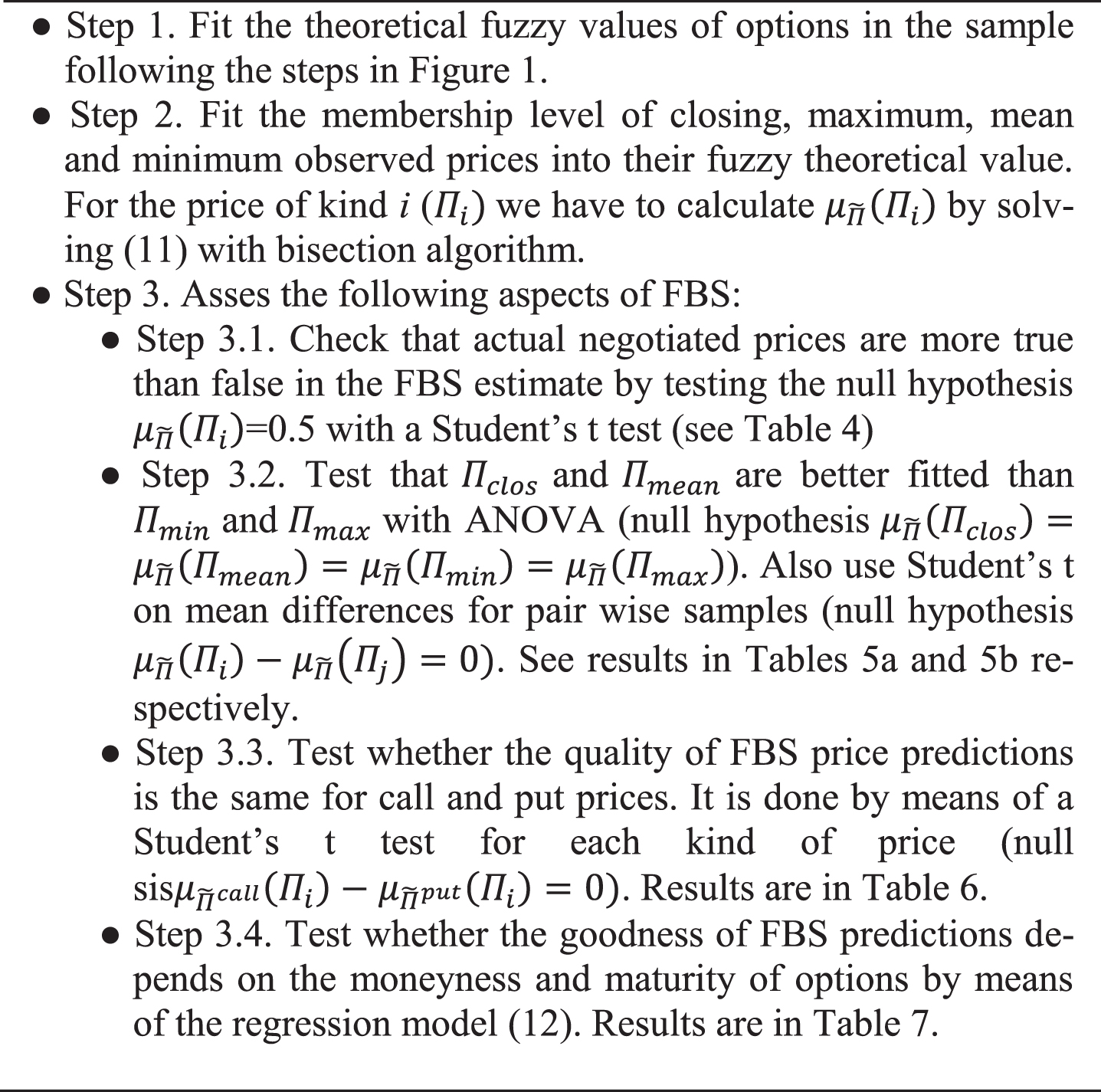
Steps to asses FBS empirically from the membership levels attained by actual option prices.

Respect the levels on which FBS fits real prices, we state if they are included in FBS prediction with a ML of at least 0.5, which is commonly considered the “cut” to consider an element nearest to be member than non-member of a fuzzy set. Lower mean MLs imply that traded prices are more false than true in FBS estimates of price and so, FBS do not make acceptable estimates of prices. To asses this issue we test whether the mean ML of a concrete kind of price is 0.5.with a Student’s t (see results are in Table 5).

Table 5

Mean values of $μ_{\tilde{Π}} (Π_{i})$ and Student’s t for the null hypothesis $μ_{\tilde{Π}} (Π_{i})$ = 0.5

	Π _close	Π _max	Π _mean	Π _min
Calls	0.60409	0.63836	0.62045	0.53958
	(6.12***)	(8.63***)	(6.78***)	(1.99**)
Puts	0.58235	0.58208	0.59010	0.58048
	(5.22***)	(5.01***)	(5.71***)	(5.04***)

Note: The value of Student’s t-ratio comes in parenthesis and *, **, *** indicates rejection of the null hypothesis $μ_{\tilde{Π}} (Π_{i})$ = 0.5 at 10%, 5% and 1% statistical significance levels.

Table 5 shows that all kind of prices are contained in their fuzzy predictions with MLs near 0.6. The exception is the minimum price of calls, where this mean ML is 0.54. The null hypothesis $μ_{\tilde{Π}} (Π_{i}) = 0.5$ is rejected with a significance level under 5% for calls minimum price and under 1% otherwise.

In Tables 6a, 6b and 7 we conduct several statistical tests on mean differences. We expect that the mean ML attained by Π_clos and Π_mean in FBS prediction will be greater than that attained by Π_max and Π_min. Table 6a shows that the results of ANOVA do not allow to accept that all call prices attain the same mean ML. However, this does not follow in the case of put prices.

Table 6a

Snedecor’s F for the null hypothesis $μ_{\tilde{Π}} (Π_{clos}) =$ $μ_{\tilde{Π}} (Π_{\max}) = μ_{\tilde{Π}} (Π_{mean})$ $= μ_{\tilde{Π}} (Π_{\min})$

	F-statistic
Calls	4.929***
Puts	0.073

Note: The value of t-ratio comes in parenthesis and *, **, *** indicates rejection of the ANOVA null hypothesis at 10%, 5% and 1% statistical significance levels.

Table 6b

Mean values and Student’s t for the null hypothesis $μ_{\tilde{Π}} (Π_{i}) - μ_{\tilde{Π}} (Π_{j}) = 0$

	Π_clos vs Π_max	Π_clos vs Π_mean	Π_clos vs Π_min
Call	– 0.0343	– 0.0164	0.0645
	(– 3.596***)	(– 1.507)	(4.184***)
Put	0.0003	– 0.0078	0.0019
	(0.025)	(– 1.019)	(0.216)
	Π_max vs Π_mean	Π_max vs Π_min	Π_mean vs Π_min
Call	0.0179	0.0988	0.0809
	(1.451)	(5.331***)	(7.336***)
Put	– 0.0080	0.0016	0.0096
	(– 0.961)	(0.108)	(1.055)

Note: The value of Student’s t-ratio comes in parenthesis and *, **, *** indicates rejection of the null hypothesis at 10%, 5% and 1% statistical significance levels.

Table 7

Mean values and Student’s t for the null hypothesis $μ_{{\tilde{Π}}^{call}} (Π_{i}) - μ_{{\tilde{Π}}^{put}} (Π_{i}) = 0$

Π _clos	Π _max	Π _mean	Π _min
0.02174	0.05628	0.03035	– 0.04090
(0.937)	(2.455***)	(1.276)	(– 1.601)

Note: The value of t-ratio comes in parenthesis and *, **, *** indicates rejection of the null hypothesis at 10%, 5% and 1% statistical significance levels.

Table 6b shows that in the case of put prices, the sign of the difference of MLs is as we expected (closing and mean prices have greater MLs than maximum and minimum prices) but in any case these differences have statistical significance. Surprisingly in call prices Π_max is better fitted than other prices and this fact has statistical significance when compare $μ_{\tilde{Π}} (Π_{\max})$ with $μ_{\tilde{Π}} (Π_{clos})$ and $μ_{\tilde{Π}} (Π_{\min})$ . Likewise, as we expected, the mean MLs of closing and mean prices are greater than that of minimum prices with a statistical significance below 1%.

Regarding the mean difference between the MLs in fuzzy estimates of calls and puts, Table 7 shows that fuzzy estimates fit better Π_clos, Π_mean and Π_max in calls than in puts whereas Π_min achieves greater MLs in put options. However we can check that these differences only have statistical significance for Π_max.

To state the influence of the degree of moneyness and the maturity on $μ_{\tilde{Π}} (Π_{i})$ we estimate a regression equation where $μ_{\tilde{Π}} (Π_{i})$ is the dependent variable and the ratio K/S and τ are the independent variables. Given that $μ_{\tilde{Π}} (Π_{i})$ must be within the interval [0,1], we estimate the following censored logistic model: $\ln (\frac{μ_{\tilde{Π}} (Π_{i})}{1 - μ_{\tilde{Π}} (Π_{i})}) = a_{1} + a_{1} \frac{K}{S} + a_{3} τ$ (12)

Table 8 shows the results of fitting (12) for all kind of call and put prices. We can check that attained MLs are positive (negative) linked with K/S in calls (puts). So, as options became more out of the money (i.e. it is less probable that will be exercised) FBS fits better the real prices. This relation reaches clear statistical significance levels in the case of closing and maximum prices of call options and in Π_clos, Π_mean and Π_min of put options.

Table 8

Value of the coefficients for the regression model (12)

		Constant	K/S	τ
Calls	Closing price	– 0.0284	0.5190	0.7724
		(– 0.097)	(1.746*)	(2.708***)
	Maximum price	0.0254	0.5907	0.1807
		(0.093)	(2.142*)	(0.686)
	Mean price	0.1553	0.4117	0.3967
		(0.533)	(1.397)	(1.406)
	Minimum price	– 0.0483	0.3593	1.4599
		(– 0.135)	(0.989)	(4.148***)
Puts	Closing price	1.1217	– 0.7246	1.0414
		(5.606***)	(– 3.735***)	(3.837***)
	Maximum price	0.8186	– 0.3061	0.4886
		(3.514***)	(– 1.351)	(1.684*)
	Mean price	0.8154	– 0.4164	1.1970
		(3.883***)	(– 2.040**)	(4.432***)
	Minimum price	0.8340	– 0.5835	1.9646
		(4.268***)	(– 3.092***)	(7.382***)

Note: The value of Student’s t-ratio comes in parenthesis and *, **, *** indicates rejection of the null hypothesis at 10%, 5% and 1% of significance levels.

Table 8 also shows that in all kind of options MLs of real prices are positive related with maturity. This relation has enough statistical entity in the case of closing and minimum prices of call options and in all kind of put prices.

4.2 Assessing the capability of the expected interval of FBS to fit real prices

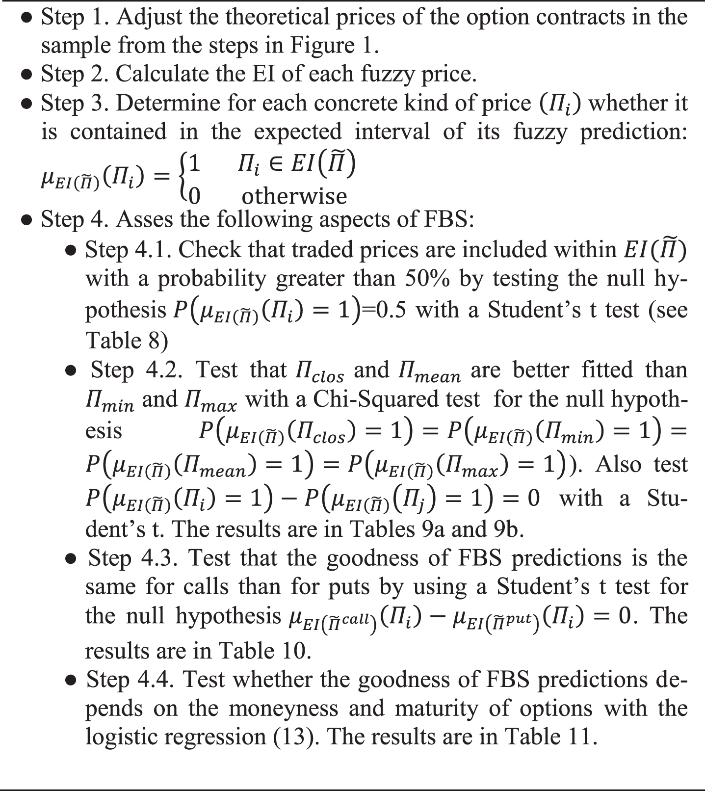
Now we assess the capability of EIs that come from FBS predictions, $EI (\tilde{Π}),$ to include actual option prices following the steps in Fig. 3. To obtain EIs we apply Simpson’s rule on (2) over (9) and (10) and, likewise, we implement (9) and (10) with a scale of eleven grades of truth, as in Table 2.

Fig.3

Steps to asses FBS empirically by means of the expected interval predictions.

We expect more frequent that any kind of real price is included within $EI (\tilde{Π})$ than not included. Likewise, we expect that Π_clos and Π_med will be more frequently within $EI (\tilde{Π})$ than extreme prices Π_max and Π_min. This analysis is made from the membership function of the crisp confidence interval $EI (\tilde{Π})$ : $μ_{EI (\tilde{Π})} (Π_{i}) = {\begin{matrix} 1 & Π_{i} \in EI (\tilde{Π}) \\ 0 & otherwise \end{matrix}$ (13)

To assess the frequency in which Π_i is included within $EI (\tilde{Π})$ we test with an Student’s t the null hypothesis $P (μ_{EI (\tilde{Π})} (Π_{i}) = 1) = 0.5$ , being P (·) the probability of the evaluated result. Notice that 0.5 is the cut to consider an outcome to be more likely than not likely. Table 9 shows that except minimum traded prices of call options, any type of option price is included in $EI (\tilde{Π})$ with frequencies above 60% and often above 65%. We reject with significance levels below 1% in practically all the cases that $P (μ_{EI (\tilde{Π})} (Π_{i}) = 1) = 0.5$ i.e., the empirical experience lead us to consider that $P (μ_{EI (\tilde{Π})} (Π_{i}) = 1) > 0.5$ .

Table 9

Observed relative frequencies of $μ_{EI (\tilde{Π})} (Π_{i}) = 1$ and Student’s t for the null hypothesis $P (μ_{EI (\tilde{Π})} (Π_{i}) = 1) = 0.5$

	Π _clos	Π _max	Π _mean	Π _min
Calls	0.66797	0.70703	0.69531	0.56641
	(5.375^***)	(6.625^***)	(6.25^***)	(2.125^**)
Puts	0.62575	0.63281	0.67578	0.69141
	(4.596^***)	(4.854^***)	(6.425^***)	(6.996^***)

Note: The value of t-ratio comes in parenthesis and *, **, *** indicates rejection of the null hypothesis at 10%, 5% and 1% statistical significance levels.

We expect that Π_clos and Π_mean should be more frequently included within $EI (\tilde{Π})$ than Π_max and Π_min. However, Table 10a shows that Chi-Square test results in call and puts do not allow rejecting that all kind of prices have the same probability to be included within $EI (\tilde{Π})$ .

Table 10a

Results of testing whether all kind of prices have the same probability to be contained in the EI of FBS prediction with a Chi-Square test

χ²-statistic
Call	4.769
Put	1.677

Note: The value of t-ratio comes in parenthesis and *, **, *** indicates rejection of the null hypothesis at 10%, 5% and 1% statistical significance levels.

Table 10b shows the results of Student’s t test for the hypothesis $P (μ_{EI (\tilde{Π})} (Π_{i}) = 1) = P (μ_{EI (\tilde{Π})} (Π_{j}) = 1)$ . In call options, Π_max is again the price better fitted but his fact only has statistical significance when compare $μ_{EI (\tilde{Π})} (Π_{\max})$ with $μ_{EI (\tilde{Π})} (Π_{\min})$ . Table 10b also shows that Π_min is the price poorer fitted by EIs and this fact always presents significant statistical levels. In the case of put options, the sign of the differences between relative frequencies of $μ_{EI (\tilde{Π})} (Π_{i}) = 1$ are not as we expected in several cases (e.g. closing prices have been included less times than minimum and minimum prices). In any case, only the difference between the relative frequencies attained by Π_clos and Π_min has real statistical significance (p-value 10%).

Table 10b

Mean value of $μ_{EI (\tilde{Π})} (Π_{i}) - μ_{EI (\tilde{Π})} (Π_{j})$ and Student’s t for the null hypothesis $P (μ_{EI (\tilde{Π})} (Π_{i}) = 1) = P (μ_{EI (\tilde{Π})} (Π_{j}) = 1)$

	Π_clos vs Π_max	Π_clos vs Π_mean	Π_clos vs Π_min
Call	– 0.0391	– 0.0273	0.1016
	(– 0.953)	(– 0.664)	(2.364***)
Put	– 0.0071	– 0.0500	– 0.0657
	(– 0.189)	(– 1.356)	(– 1.789*)
	Π_max vs Π_mean	Π_max vs Π_min	Π_mean vs Π_min
Call	0.0117	0.1406	0.1289
	(0.290)	(3.308***)	(3.032***)
Put	– 0.0430	– 0.0586	– 0.0156
	(– 1.168)	(– 1.601)	(– 0.434)

Note: The value of t-ratio comes in parenthesis and *, **, *** indicates rejection of the null hypothesis at 10%, 5% and 1% statistical significance levels.

Regarding the difference between the frequency in which call and put prices are within $EI (\tilde{Π})$ , Table 11 shows, as Table 7 that FBS fits better Π_clos, Π_mean and Π_max in calls than in puts whereas Π_min is better predicted in put options. We also can check that these differences only have statistical significance in the case of maximum and minimum prices.

Table 11

Difference between the relative frequency of $μ_{EI (\tilde{Π})} (Π_{clos}) = 1$ , $μ_{EI (\tilde{Π})} (Π_{\max}) = 1$ , $μ_{EI (\tilde{Π})} (Π_{\max}) = 1$ , $μ_{EI (\tilde{Π})} (Π_{med}) = 1$ and $μ_{EI (\tilde{Π})} (Π_{\min}) = 1$ of calls and puts

Π _clos	Π _max	Π _mean	Π _min
0.0422	0.0742	0.0195	– 0.1250
(1.061)	(1.893*)	(0.506)	(– 3.130***)

Note: The value of t-ratio comes in parenthesis. *, **, *** indicates rejection of the null hypothesis at 10%, 5% and 1% statistical significance levels.

We now analyze the influence of the degree of moneyness and the maturity on $μ_{EI (\tilde{Π})} (Π_{i})$ . So we fit a logistic regression where $μ_{EI (\tilde{Π})} (Π_{i})$ is the dependent variable, which takes values on {0, 1} and K/S and τ are again the explanatory variables. $\ln (\frac{μ_{EI (\tilde{Π})} (Π_{i})}{1 - μ_{EI (\tilde{Π})} (Π_{i})}) = a_{1} + a_{1} \frac{K}{S} + a_{3} τ$ (14)

Table 12 shows the results of fitting (14) for all type of prices and options. We can check again that $μ_{EI (\tilde{Π})} (Π_{i})$ has a positive relation with maturity. This relation has solid statistical significance practically for any kind of price and/or option. In call prices and for closing, maximum and minimum prices we also detect a positive relation between $μ_{EI (\tilde{Π})} (Π_{i})$ and K/S whose significance level is above 5%. On the other hand, the sign of the relation between $μ_{EI (\tilde{Π})} (Π_{i})$ and K/S is not clear for put prices. This sign is negative for maximum and minimum prices and also positive for closing and mean prices. In any case, those contradictory relations have not relevant statistical significance levels.

Table 12

Fitted coefficients for the logistic regression model (14)

		Constant	K/S	τ
Calls	Closing price	– 5.4942	5.7277	3.8487
		(– 2.407^***)	(2.487^***)	(1.787^*)
	Maximum price	– 4.6484	5.4831	0.9100
		(– 2.014^**)	(2.348^***)	(0.412)
	Mean price	– 4.6766	5.1098	3.2728
		(– 2.023^**)	(2.189^**)	(1.495)
	Minimum price	– 3.8037	3.4200	4.7777
		(– 1.777*)	(1.585)	(2.330^***)
Puts	Closing price	1.0982	– 1.7111	6.9512
		(0.753)	(– 1.182)	(3.684^***)
	Maximum price	– 0.5142	0.5478	3.4942
		(– 0.365)	(0.395)	(1.884^*)
	Mean price	– 0.5628	0.1699	6.9848
		(– 0.380)	(0.116)	(3.636^***)
	Minimum price	0.9200	– 2.2252	11.2752
		(0.602)	(– 1.461)	(5.668^***)

Note: The value of t-ratio comes in parenthesis and *, **, *** indicates rejection of the null hypothesis at 10%, 5% and 1% statistical significance levels.

5 Conclusions

This paper exposes the fuzzyfied extension of Black and Scholes model [1], (FBS), developed in [38 –40] and proposes a suitable way to fit empirically subjacent asset price, free interest rate and volatility to evaluate FBS. Whereas fuzzy stock price and discount rate are obtained directly from empirical data, volatility is fitted by a fuzzy regression model similar to [26]. It links implied volatility with grade of moneyness and maturity of the options. In our opinion, it may be of interest investigating if other fuzzy volatility models as [6 , 23] allow obtaining better empirical results. Likewise, we think that granular computing (see for several perspectives [10 , 31– 33]) is a very promising field to model financial time series as it is shown in [22, 23]. So, future applications of granular computing on option pricing field could be fruitful.

We also assess the performance of FBS to predict traded prices (closing, maximum, mean and minimum) in two ways. The first one is based on the analysis of the membership levels (MLs) of real prices into fuzzy estimates. The second is developed from the relative frequency in which traded prices are included into the expected interval (EI) of FBS. We can synthesize the results as follows:

Both testing procedures reveal that FBS predicts reasonably well all types of market price. FBS contains all kind of prices with MLs greater than 0.5 (i.e, they are more true than false) whereas the EI of FBS contains with probabilities greater than 50% those prices.

Minimum and maximum prices can be considered as extreme values whereas closing and mean prices can be assimilated to representative prices. So, it is reasonable to expect that the extreme prices must be worst fitted than those more representative. This hypothesis is only proved for the minimum price of call options. In fact, it seems that in call options FBS fits better maximum prices than kind of prices whereas in put options we cannot reject that all type of prices are equally well fitted.

Our analysis indicates that FBS fits with approximately equal precision in calls and puts, closing and mean prices. On the other hand, it seems clear that FBS tends to adjust better maximum (minimum) prices in call (put) contracts.

The results of fitting the regression models (12) and (14) reveal that option moneyness and expiration date are relevant to explain the capability of FBS to fit actual prices. We have checked that the closeness of FBS estimates to actual prices increases with the maturity of the option. In (12) that positive relation is statistically significant for closing and minimum prices of call options and in all kind of put prices. This pattern is also detected in the regression model (14).

The option moneyness has been measured with the ratio strike price/price (K/S). We have checked that this ratio may be positive (negative) linked with the closeness of actual call (put) prices and their fuzzy estimates. That is to say, FBS seems to work better in options that are more out of the money. In the case of call prices this relation is not especially clear when estimating (12). On the other hand, we have found a clear statistical significance when analyzing the capability of $μ_{EI (\tilde{Π})} (Π_{i})$ to include closing, maximum and mean call prices. In the case of put options, the negative relation of K/S with the goodness of FBS predictions is easy to accept in (12) but it is not clear at all in the regression model (14).

In our opinion, the main contribution of this paper is that test empirically the closeness of FBS developed in [38 –40] to actual market data. As we have shown in the introduction, there is a wide research field that consists in adapting option pricing models to fuzzy data but also a lack of empirical studies on this topic. So, a natural extension of this research may extend the empirical evidence about FBS to option markets of other countries. Another future research direction may consist in testing with real data other fuzzy option pricing models that are supported from more sophisticated hypothesis on the stochastic process that governs subjacent asset [10 , 42] or are developed for less usual option styles than European or American [36, 37].

Footnotes

Notice that since 2016, in Eurozone, the interest rates due to the monetary policy of European Central Bank are negative in all short term monetary markets.

Acknowledgments

Author thanks the helpful comments of anonymous reviewers.

References

Black

and Scholes

, The pricing of options and corporate liabilities, Journal of Political Economy81(3) (1973), 637–654.

Buckley

J.J.

, Fuzzy statistics: Hypothesis testing, Soft Comput9(7) (2005), 512–518.

Buckley

J.J.

and Eslami

, Pricing options, forwards and futures using fuzzy set theory, In Fuzzy Engineering Economics with Applications, Springer Berlin Heidelberg, 2008, pp. 339–357.

Buckley

J.J.

and Qu

, On using α-cuts to evaluate fuzzy equations, Fuzzy Sets and Systems38(3) (1990), 309–312.

Buckley

J.J.

and Qu

, Solving fuzzy equations: A new solution concept, Fuzzy Sets and Systems39(3) (1991), 291–301.

Capotorti

and Figá-Talamanca

, On an implicit assessmentof fuzzy volatility in the Black and Scholes environment, Fuzzy Sets and Systems223 (2013), 59–71.

Carlsson

and Fullér

, A fuzzy approach to real option valuation, Fuzzy sets and systems139(2) (2003), 297–312.

Chen

, Chen

, Zhou

and Liu

, Optimizing h value for fuzzy linear regression with asymmetric triangular fuzzy coefficients, Engineering Applications of Artificial Intelligence47 (2016), 16–24.

Chrysafis

K.A.

and Papadopoulos

B.K.

, On theoretical pricing of options with fuzzy estimators, Journal of Computational and Applied Mathematics223(2) (2009), 552–566.

10.

Dubois

and Prade

, Bridging gaps between several forms of granular computing, Granular Computing1(2) (2016), 115–126.

11.

Dumas

, Fleming

and Whaley

R.E.

, Implied volatility functions: Empirical tests, The Journal of Finance53(6) (1998), 2059–2106.

12.

Figa-Talamanca

, Guerra

M.L.

and Stefanini

, Market application of the fuzzy-stochastic approach in the heston option pricing model, Finance a Uver62(2) (2012), 162.

13.

Fiorentini

, León

and Rubio

, Estimation and empirical performance of Heston’s stochastic volatility model: The case of a thinly traded market, Journal of Empirical Finance9 (2002), 225–255.

14.

Guerra

M.L.

, Sorini

and Stefanini

, Option price sensitivities through fuzzy numbers, Computers & Mathematics with Applications61(3) (2011), 515–526.

15.

Heilpern

, The expected value of a fuzzy number, Fuzzy Sets and Systems47 (1992), 81–86.

16.

Heston

S.L.

, A closed-form solution for options with stochasticvolatility with applications to bond and currency options, Review of financial studies6(2) (1993), 327–343.

17.

Ishibuchi

and Nii

, Fuzzy regression using asymmetric fuzzy coefficients and fuzzified neural networks, Fuzzy Sets and Systems119 (2001), 273–290.

18.

Jiménez

and Rivas

J.A.

, Fuzzy number approximation, International Journal of Uncertainty, Fuzziness and Knowledge-Based Systems6(01) (1998), 69–78.

19.

Liu

, Gegov

A.E.

and Cocea

, Rule based systems: A granular computing perspective, Granular Computing1(4) (2016), 259–274.

20.

Loia

, D’Aniello

, Gaeta

and Orciuoli

, Enforcing situation awareness with granular computing: A systematic overview and new perspectives, Granular Computing2(1) (2016), 127–143.

21.

MacBeth

J.D.

and Merville

L.J.

, An empirical examination of the black-scholes call option pricing model, The Journal of Finance34(5) (1979), 1173–1186.

22.

Maciel

, Ballini

and Gomide

, Evolving granular analytics for interval time series forecasting, Granul Comput1 (2016), 213–224.

23.

Maciel

, Gomide

and Ballini

, Evolving fuzzy-GARCH approach for financial volatility modeling and Forecasting, Computational Economics48(3) (2016), 379–398.

24.

Merton

R.C.

, Applications of option-pricing theory: Twenty-five years later (digest summary), American Economic Review88(3) (1998), 323–349.

25.

Mixon

, The implied volatility term structure of stock index options, Journal of Empirical Finance14(3) (2007), 333–354.

26.

Muzzioli

, Ruggieri

and De Baets

, A comparison of fuzzy regression methods for the estimation of the implied volatility smile function, Fuzzy Sets and Systems266 (2015), 131–143.

27.

Muzzioli

and De Baets

, Fuzzy approaches to option price modeling, IEEE Transactions on Fuzzy Systems25(2) (2017), 392–401.

28.

Nowak

and Romaniuk

, Computing option price for Levy process with fuzzy parameters, European Journal of Operational Research201(1) (2010), 206–210.

29.

Nowak

and Romaniuk

, A fuzzy approach to option pricing in a Levy process setting, International Journal of Applied Mathematics and Computer Science23(3) (2013), 613–622.

30.

Nowak

and Romaniuk

, Application of Levy processes and Esscher transformed martingale measures for option pricing in fuzzy framework, Journal of Computational and Applied Mathematics263 (2014), 129–151.

31.

Peters

and Weber

, DCC: A framework for dynamic granular clustering, Granular Computing1(1) (2016), 1–11.

32.

Sánchez

M.A.

, Castro

J.R.

, Castillo

, Mendoza

, Rodríguez-Diaz

and Melin

, Fuzzy higher type information granules from an uncertainty measurement, Granular Computing2(2) (2016), 95–103.

33.

Skowron

, Jankowski

and Dutta

, Interactive granular computing, Granular Computing2(1) (2016), 95–113.

34.

Sfiris

D.S.

and Papadopoulos

B.K.

, Non-asymptotic fuzzy estimators based on confidence intervals, Information Sciences279 (2014), 446–459.

35.

Tanaka

, Fuzzy data analysis by possibility linear models, Fuzzy Sets and Systems24 (1987), 363–375.

36.

Thavaneswaran

, Appadoo

S.S.

and Frank

, Binary option pricing using fuzzy numbers, Applied Mathematics Letters26(1) (2013), 65–72.

37.

Wang

, He

and Li

, Compound option pricing under fuzzy environment, Journal of Applied Mathematics (2014).

38.

H.C.

, Pricing European options based on the fuzzy pattern of Black– Scholes formula, Computers & Operations Research31(7) (2004), 1069–1081.

39.

H.C.

, Using fuzzy sets theory and Black– Scholes formula to generate pricing boundaries of European options, Applied Mathematics and Computation185(1) (2007), 136–146.

40.

, Xu

, Li

and Zhang

, A study of Greek letters of currency option under uncertainty environments, Mathematical and Computer Modelling51(5) (2010), 670–681.

41.

Yoshida

, The valuation of European options in uncertain environment, European Journal of Operational Research145(1) (2003), 221–229.

42.

Zhang

L.H.

, Zhang

W.G.

, Xu

W.J.

and Xiao

W.L.

, The double exponential jump diffusion model for pricing European options under fuzzy environments, Economic Modelling29(3) (2012), 780–786.

43.

Zmeškal

, Application of the fuzzy– stochastic methodology to appraising the firm value as a European call option, European Journal of Operational Research135(2) (2001), 303–310.

44.

Zmeškal

, Generalised soft binomial American real option pricing model (fuzzy– stochastic approach), European Journal of Operational Research207(2) (2010), 1096–1103.

An empirical assestment of fuzzy Black and Scholes pricing option model in Spanish stock option market

Abstract

Keywords

1 Introduction

2 Functions of fuzzy variables and fuzzy regression

3.1 Pricing European options by evaluating Black and Scholes model with fuzzy parameters

Table 3 Results of fitting σ = a 0 + a 1 k s + a 2 ( k s ) 2 + a 3 τ for the options on IBEX35 negotiated in MEFFSA at t = 2/28/2017

Footnotes

Acknowledgments

References

Table 3
Results of fitting $σ = a_{0} + a_{1} \frac{k}{s} + a_{2} {(\frac{k}{s})}^{2} + a_{3} τ$ for the options on IBEX35 negotiated in MEFFSA at t = 2/28/2017