Design of computer interactive system for sports training based on artificial intelligence and improved support vector

Abstract

At present, there is less software related to sport technical behavior recognition, and there are few studies on the classification and identification of detailed actions. By introducing computer technology to analyze the efficiency and regularity of sports, not only the characteristics of athletes can be excavated, but also the visibility and dynamic tracking of sport training can be provided. The process of sports education is a fast and complex systematic process. Through the interactive system of physical education, we can use different methods to collect sports data and make a comparative analysis of athletes’ movements. Through the data mining of the relationship between athletes’ physiological indexes and sports load, the unreasonable link in sports training can be avoided. Also, in sports training, we can use computer vision and modern biomechanics to construct a virtual sports education situation. With the classification accuracy as the fitness function, this paper collects the data through the network database, and returns the corresponding sport training parameters on this basis. The results showed that the accuracy of the model was nearly 98%, which met the actual demand. Therefore, the development of sports education assistant system can provide strong support for the process control of sports training and education.

Keywords

Support vector improved model computer interactive system recognition algorithm

1 Introduction

The research on human behavior recognition can be traced back to the 1990s [1]. As an important research field of ubiquitous computing, the role of human behavior recognition is to monitor and sense the activity state, exercise intensity and energy consumption of the human body. With the development of science and technology, the recognition of human behavior can be used as a basis to provide support for various upper-level applications. Moreover, with the improvement of people’s living standards, its application in the fields of smart home, elderly guardianship, patient monitoring, athlete rehabilitation and other aspects gradually began to appear [2].

The ways to obtain human behavior data are mainly divided into two types based on vision and wearable sensing networks [3]. Vision-based human behavior recognition is suitable for large-scale occasions with high security requirements such as banks, supermarkets, and schools. Due to factors such as expensive recording equipment, complex identification algorithms, limited monitoring range, and easy disclosure of the privacy of the monitored person, it is limited in the application of the field of behavior recognition with high intelligence and energy consumption requirements. With the continuous development of wireless communication technology, sensortechnology and embedded computing technology, wireless sensor networks and body area network technologies have begun to appear, and behavior recognition methods based on wearable sensor networks have begun to attract people’s attention. The method is to obtain a series of data such as acceleration data, environmental variables and physiological signals when the human body moves by wearing various types of sensors in different parts of the human body. Moreover, after analyzing and processing such data, it can be used to judge the motion state of the human body [4].

Human-based behavior recognition requires comprehensive use of machine vision for target detection, biometric analysis, biometric classification method research and other related professional knowledge, which has interdisciplinary and high comprehensive characteristics. Since the human body belongs to a non-rigid object, the mathematical modeling, feature selection, feature extraction and compression, feature classification and feature recognition of the target human body are relatively difficult. In literature [5], a method for detecting anomalous behavior based on motion direction is proposed. It uses block motion directions to describe different actions and uses support vector machines.

The target behavior analysis relies on computer vision analysis technology, which is mainly divided into three levels of analysis processing at the bottom, middle and high levels. The middle and bottom layers mainly include motion detection, tracking and classification of targets [6]. Moreover, the prediction of the target behavior category belongs to the high-level behavior of the target behavior recognition, for example, to determine whether the current target behavior has an abnormal behavior.

The athletes’ various training actions and competition actions not only have certain ornamental characteristics, but also have certain dangers. Moreover, some details of the action will lead to an increase in the probability of athletes’ injury, and some bad habits will also have an impact on the athlete’s training and competition.

2 Related work

At present, the recognition of human behavior includes two methods, namely, a vision-based sensor network and a wearable-based sensor network [7]. Vision-based behavior recognition mainly uses high-frequency cameras for image acquisition and analysis. It not only recognizes human behavior, but also performs facial expression recognition, gesture recognition, etc. [8], and is widely used in security fields (such as intrusion detection) and human-computer interaction.

For example, Microsoft launched the Kinect somatosensory device in 2010. It does not require any controllers, just captures and recognizes the player’s actions in 3D space through the camera, which allows the player to participate in the game. H. Qian et al. used a visual-based approach to identify behaviors such as walking, jumping, standing, sitting, and falling, and obtained a higher accuracy of behavior recognition [9]. At present, there are three main problems in vision-based behavior recognition. Firstly, visual-based behavior recognition is easy to cause the leakage of the monitored person’s privacy. However, not all of the monitored persons are willing to record their own actions at the moment by the video equipment. Secondly, in order to record the daily behavior image of the monitored person as comprehensively as possible, the range of the activity of the monitored person must be captured around the video device, so the monitoring range based on the abnormal behavior of the video is limited. In addition, video recording equipment is relatively expensive, and video processing calculations are complex, which hinders the development of vision-based behavior recognition technology [10].

With the continuous development of microelectromechanical systems (MEMS) and wireless sensor networks (WSN), human behavior related data such as motion data (position, acceleration), environmental variables (temperature, humidity), and physiological parameters (heart rate, ECG signals) can be obtained by wearable wireless sensors. Moreover, the wearable wireless sensor is increasingly used in behavior recognition research because of its small size, light weight, low energy consumption and convenient carrying [11].

At present, many human body behavior recognition systems based on acceleration sensors have been proposed [12]. Some of these studies classify different types of physical activities by analyzing acceleration signals, such as going upstairs, going downstairs, etc.; Moreover, there are some studies used to identify daily activities such as lying, sitting, standing, walking, running, etc. in life; Minnen et al. used acceleration data to identify recurring activities such as hammering, sanding, drilling, etc.; Giansanti and Narayanan et al. used this accelerometer-based anomaly behavior recognition system for fall detection and prevention in the elderly. In order to improve the accuracy of behavior recognition, early behavioral recognition systems based on wearable sensor networks usually need to fix multiple sensors in different parts of the human body for data collection, such as waist, thigh, chest, arms, back, wrist and ankles, etc.

In the literature [13], five two-axis accelerometers are fixed on the ankle, thigh, wrist, arm, and buttocks of the human body to obtain human behavior data. Although the behavior data obtained by it is more comprehensive, the system consumes a large amount of energy, has a large amount of calculation, and the wearer’s comfort is poor, which seriously hinders the daily life of human beings. Therefore, at this stage, more and more researchers are studying the behavior of individual acceleration sensors. Chernbumroong and Atkins fixed an accelerometer at the wrist and collected acceleration data to distinguish five behaviors of sitting, standing, lying, walking, and running [14]. Also distinguishing these five behaviors, Choi and LeMay fixed a Shimmer node at the waist to collect acceleration data [15]. In the literature [16], the recognized behavior includes standing, walking, running, going up and down the stairs. Because the actions involved are leg movements, the sensor nodes are fixed to the legs.

As a new research field, the human behavior recognition system based on wearable sensor network has achieved unprecedented development, but there are still some problems that researchers need to solve. First of all, by reading a large amount of literature, it is learned that the current research on human behavior mainly focuses on normal daily behaviors such as walking, running, sitting, lying down, going up and down stairs, taking elevators, but the attention to abnormal behavior is relatively small, and most of them are mostly concentrated on the fall monitoring of the elderly. If the behavioral recognition based on wearable sensor networks is to be extended to prison management and military fields other than smart home, elderly guardianship, medical rehabilitation, the identification of abnormal behaviors such as fights should also attract attention. Secondly, the sensor node that collects human behavior data has its endurance capability provided by its own battery. Due to the small size of the sensor node, the battery life is limited. Moreover, today’s behavior recognition system has large data collection and large complexity of feature space calculation, which leads to large system energy consumption, short system life time and poor real-time system. Therefore, how to effectively extract behavioral data features while ensuring the accuracy of behavior recognition, real-time and low-power behavior recognition systems should also be concerned [17].

In addition, the selection of behavior recognition algorithms and their parameters will also affect the power consumption and real-time performance of the system. Therefore, how to construct an efficient behavior recognition algorithm is also worthstudying.

3 Target recognition algorithm

The identification of targets is usually based on statistical methods, and the difficulty of statistical methods is that it often involves dimensionality problems. In all the information that expresses the target, the algorithm hopes to remove the redundant information and retain the feature information that can represent the target as little as possible. That is, in the case where the target is not distorted, the less the data describing the target, the better, that is, the dimension of the target description information is considered to be reduced. Moreover, reducing the dimension of the target information is often a difficult point to solve the problem in practice [18]. The reduction of the target dimension is actually to reduce the high dimensionality of the target information amount to a low-dimensional space through a certain projection. The Fisher method is to project the target high-dimensional information into a one-dimensional space and compress the target image to a spatial straight line while ensuring that the information required by the target is not distorted. Then, the most appropriate boundary is found, which can distinguish between different types of targets. The main function of the algorithm is to find the optimal projection direction so that the distance between all the target classes to be classified is maximized when the target is mapped onto the line. The algorithm is described below [19]:

The average values of the samples to be classified in the high-dimensional feature space are as follows: $Φ_{i} = \frac{1}{n_{i}} \sum_{x_{k} \in X_{i}} x_{k}, i = 1, 2, \dots, N$ (1)

The projection algorithm is: $Φ_{i} = w^{T} φ_{i}$ (2)

The average of the projected objects in the projected one-dimensional space: $φ_{i} = \frac{1}{n_{i}} \sum_{y_{k} \in Y_{i}} y_{k}, i = 1, 2, \dots, N$ (3)

The distance between classes of the target sample in the one-dimensional feature space is expressed as: $L_{i}^{2} = \sum_{y_{k} \in Y_{i}} {(y_{k} - m_{i})}^{2}$ (4)

The greater the distance between the two classes, the smaller the intra-class dispersion of each sample, the more it can meet the mapping needs. The fisher criterion function is defined as [20]: $\begin{matrix} J_{F} (w) = \frac{{| φ_{1} - φ_{2} |}^{2}}{L_{1}^{2} + L_{2}^{2}} = \\ \frac{{∥ w^{T} M_{1} - w^{T} M_{2} ∥}^{2}}{w^{T} (\vec{L_{1}} + \vec{L_{2}}) w} = \\ \frac{w^{T} \vec{L_{b}} w}{w^{T} \vec{L_{w}} w} \end{matrix}$ (5)

When the maximum value of J_F is taken, the mapping variable w^* is the best projection direction. $w^{*} = \vec{L_{w}} (Φ_{1} - Φ_{2})$ (6)

φ₁, φ₂ are different two categories, and L₁, L₂ are the corresponding inter-class distance.

In general, the procedure for solving the fisher algorithm is [21]:

Solving the variance between classes Φ_i

Solving all types of internal dispersion matrices: $\vec{L_{i}} = \sum (x_{k} - Φ_{i}) {(x_{k} - Φ_{i})}^{T}$ (7)

Calculating the total dispersion within the class: $\vec{L_{w}} = \vec{Φ_{1}} + \vec{Φ_{2}} + \dots + \vec{Φ_{n}}$ (8)

Calculating ${\vec{Φ_{w}}}^{- 1}$

Calculating $w^{*} = \vec{L_{w}} (Φ_{1} - Φ_{2})$ (9)

When using the Fisher algorithm, if the sample is linearly separable, the sample with dimensionality reduction after the projection direction has higher separability. Moreover, the distance between the classes increases, and the distance within the class decreases. The following conditions do not apply to fisher [22]:

When L₁ = L₂,w^* = 0, at this time, the sample is inseparable;

When L₁ ≠ L₂, the sample is not necessarily linearly separable;

When $\vec{L_{w}}$ is irreversible, the sample is not necessarily linearly separable.

4 Improved support vector machine

Support Vector Machine (SVM) is based on the framework of statistical learning theory and structural risk minimization. For a limited sample, based on its limited information, the model is constructed by translating the actual problem dimensions to avoid the dimensionality catastrophe problem and classifying each sample. It is another new research hotspot of data-based machine learning after neural network research.

Support vector machines evolved through the theory of optimal classification planes. This section will explain the basic operation process of the support vector machine by classifying the two types of samples.

(1) Support Vector Machines

As shown in Fig. 1, C₁, C₂ are two types of separable samples, and line H can completely separate the two types of samples. Among them [23]:H : g (x) = x · w + b

Fig.1

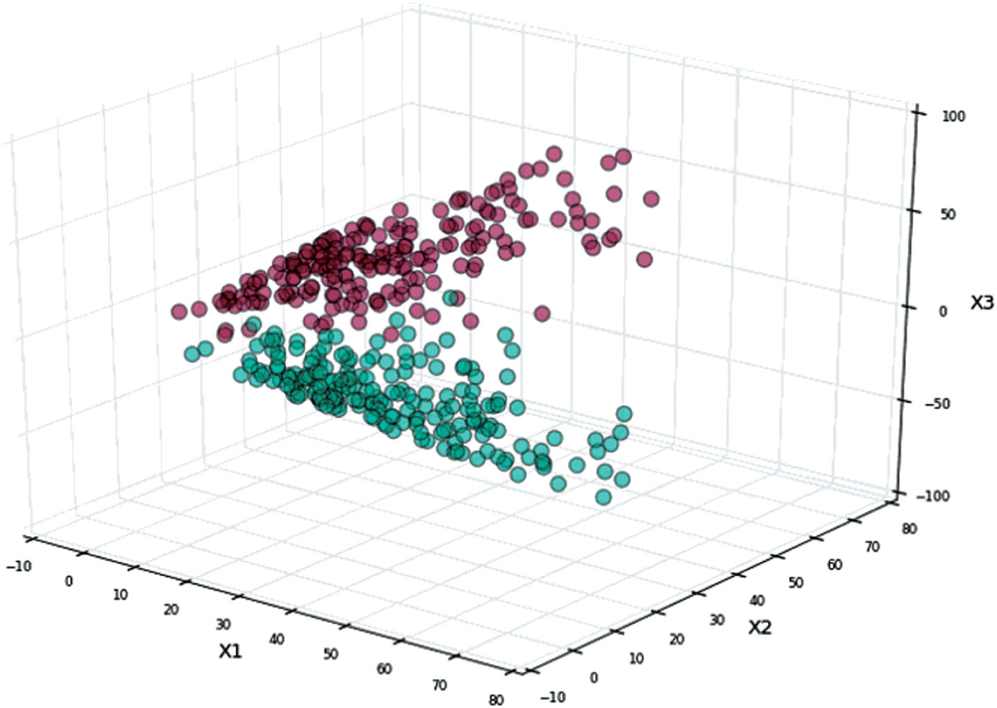
Data to be classified.

C₁, C₂ are called linear separable, otherwise they are nonlinearly separable. As can be seen from the figure, if the sample x_i belongs to the C₁ class, then x_i · w + b > 0,

When it belongs to C₂ class, x_i · w + b < 0°

Thus, it is determined whether the current sample belongs to the class by whether g (x) = x · w + b is greater than 0.

(2) Search process of optimal classification surface

There are two types of samples as shown in Fig. 2, where H is the classification line, and H₁, H₂ are the straight lines of the classes closest to the classification line and parallel to them, and the distance between them is called the classification margin. The two types of classification lines that are correctly separated and have the largest classification interval are called the optimal classification line, that is x · w + b = 0.

Fig.2

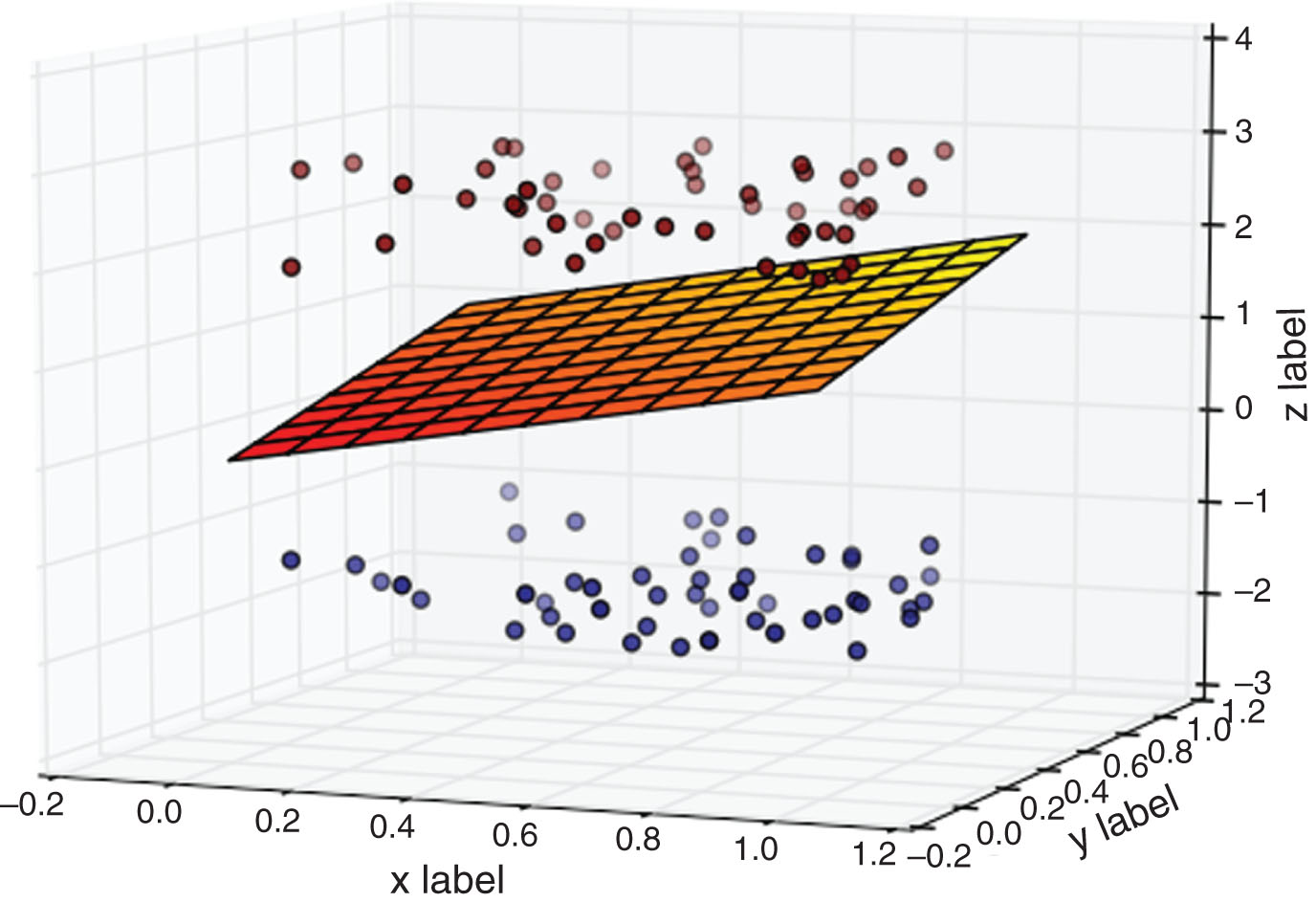
Schematic diagram of classification.

Linear separable sample set $(x_{i}, y_{i}), i = 1, \dots, n, x \in R^{d}, y \in {+ 1, - 1}$

satisfies [24]: $y_{i} [(w \cdot x_{i}) + b] - 1 ⩾ 0, i = 1, \dots, n$ (10)

Among them, the classification interval is 2/ -∥ w ∥. To maximize the classification interval, we need to minimize ∥w ∥ ²2, and the classification surface at this time is called the optimal classification surface.

The sample H₁, H₂ are called the support vector.

The dual problem is solved by the Lagrange optimization method for the appeal problem. For constraints [25]: $\sum_{i = 1}^{n} y_{i} α_{i} = 0, α_{i} ⩾ 0, i = 1, \dots, n$ (11)

The maximum value of the following variables is solved: $Q (α) = \sum_{i = 1}^{n} α_{i} - \frac{1}{2} \sum_{i, j = 1}^{n} α_{i} α_{j} y_{i} y_{j} (x_{i} \cdot x_{j})$ (12)

This formula is a problem of optimization for formula (10). Among them, α_i is the Lagrange operator corresponding to Equation (10). Among the obtained solutions, the sample of α_i which is not zero is the support vector. The optimal classification function is: $\begin{matrix} f (x) = sgn {(w \cdot x) + b} \\ = sgn {\sum_{i = 1}^{n} α_{i}^{*} y_{i} (x_{i} \cdot x) + b^{*}} \end{matrix}$ (13)

Among them, b^* is the classification threshold and is obtained when any of the support vectors satisfies the formula (11) as 0.

(3)Support vector machine extension

For the classification of high-dimensional data, the basic idea of SVM is to find the optimal hyperplane classification surface in high-dimensional space under the condition that the sample is linearly separable and classify and identify the data through the classification.

Since the value of the optimization function and the classification function involve the inner product between the training functions, when constructing the high-dimensional feature space, the algorithm only involves the dot product between the samples. For high-dimensional spaces, a linear transformation can be achieved by using the appropriate inner product function K (x_i · x_j), which is called a kernel function. Then the optimization objective function becomes $Q (α) = \sum_{i = 1}^{n} α_{i} - \frac{1}{2} \sum_{i, j = 1}^{n} α_{i} α_{j} y_{i} y_{j} K (x_{i} \cdot x_{j})$ (14)

The classification function is changed to $\begin{matrix} f (x) = sgn {(w \cdot x) + b} \\ = sgn {\sum_{i = 1}^{n} α_{i}^{*} y_{i} K (x_{i} \cdot x) + b^{*}} \end{matrix}$ (15)

In the above algorithm, it is assumed that the samples are completely correctly classified. However, in practical problems, it is necessary to seek a balance between experience risk and promotion performance, and appropriately allow the existence of misclassified samples. Moreover, the relaxation factor ξ_i is introduced, and when ∥w ∥ ² is minimized, the penalty factor $C \sum_{i = 1}^{n} ξ_{i}$ is introduced. The general form of support vector machine is: $\begin{matrix} Maximize : Q (α) = \sum_{i = 1}^{n} α_{i} - \\ \frac{1}{2} \sum_{i, j = 1}^{n} α_{i} α_{j} y_{i} y_{j} K (x_{i} \cdot x_{j}) \end{matrix}$ (16) $\begin{matrix} s . t . : \sum_{i = 1}^{n} y_{i} α_{i} = 0 \\ 0 ⩽ α_{i} ⩽ C i = 1, \dots, n \end{matrix}$

The performance of a support vector machine is usually determined by its kernel function based feature space and hyperplane classifier. Moreover, when it was first proposed, it was mainly used to solve two types of groups to be classified. The main task of constructing the support vector machine is to select the appropriate kernel function, and in the case of ensuring the error rate and the minimum empirical risk, the classification hyperplane is sought to make it possible to present each group to be classified well in the feature space. However, in the actual situation, the population to be classified is usually in more than two categories.

There are currently k categories to be classified, and there are two ways to classify them: One-Against— One, OAO, One— Against-All, OAA. OAO first classifies the current group to be classified, and all the remaining groups as one, and so on, until the last two categories are classified. Each class is subordinate to a region, and its essence is a function optimization problem for multiple classes of targets. OAA classifies each group as a separate category. Moreover, it still classifies two types of targets, one is the target to be classified, and the remaining samples are one.

The OAO model Vapnik was proposed in 1995 and is based on traditional classification methods. There are C class to be classified, and C SVMs are required. When L samples are trained, the input vector is: $T_{xy} = {(x_{1}, y_{1}), \dots, (x_{L}, y_{L})}$ (17)

x_i∈ X, y_i ∈ Y = { 1, 2, ⋯ , c }, x_i is a training sample and y_i is a sample marker. In the OAO model, if one of the data is accepted by the existing category in the current classification, the remaining categories will not accept the data. In the case of an error, after a certain class is rejected by the class, the other classes also do not accept the data, and eventually the data is not accepted by any class. In addition, the calculation of this method is extremely large, and the application is actually difficult. Vapnik proposed improvements to the traditional OAA in 1998. The specific method is that the current classification to be classified is 1, and the remaining classes are marked as -1. This construction method makes the classification to be associated with each support vector machine before being judged to be a certain class and allows it to be accepted after missing the correct classification. Therefore, the decision rule is usually a matching class when the maximum value of the output value is taken at the position of the support vector machine.

Another construction method is a one-to-many paired join. This method takes a classification process for every two classes and requires a total of c (c - 1)/ - 2 classifiers. Each classifier classifies data from two pre-classified categories. Moreover, each classifier votes on which class the unknown data belongs to, and the class that gets the most votes is judged as the class.

Support vector machines based on the OAA model will be used in this section. The following figure shows the classification and identification of the database class behavior in this section. The experimental results show that the SVM classifier using the OAA model can basically classify most of the categories in this section of the database. Figure 3 is a classification test of the shape information of three different types of behavior in this section. First, the behavior Walk is taken as a class, and Crouch and Fall are identified as a class. The classification result is shown in Fig. (a). The Crouch and Fall are then classified, and the results are shown in Fig. (b). The results show that the feature variables used in this section can better describe the target behavior, and the classification effect is obtained by the classifier.

Fig.3

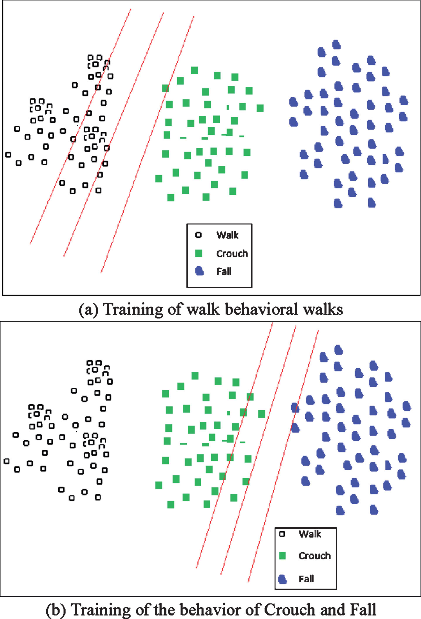
Classification results for walk, crouch, and fall. (a) Training of walk behavioral walks, (b) Training of the behavior of crouch and fall.

Table 1 is the statistics of the average behavior classification accuracy of the SVM based on the OAA model for the database based on the silhouette contour shape information.

Table 1

Statistics of the correct rate of database behavior classification based on OSA model SVM

Template	Action
	Sit(%)	Walk(%)	Run(%)	Walk(%)	Fall(%)
Rec.ratio	89.816	89.301	52.324	90.846	94.863

From the statistics of the above table, the support vector machine based on OAA model used in this paper has a good effect on the classification of the feature variables of the shape information, especially the recognition of the abnormal behavior Fall, which has a high accuracy.

5 Model construction and performance analysis

In order to study the effectiveness of the algorithm in this study, we now build a model case for analysis. This study takes the badminton net front hook diagonal as an example for analysis. In order to establish the PSO-SVM network front diagonal model, firstly, the training set and test set should be extracted from the obtained raw data. Then, this paper conducts certain data analysis and preprocessing, trains the PSO SVM network with the training set, and finally uses the obtained model to test and analyze the test data.

In Fig. 4, for the collected 240 sets of data, 180 sets of data are used to train the PSO-SVM net front hook diagonal model, and 60 sets of data are used to test the model. Among the 180 pieces of training data, 120 groups are successful data in front of the net and 75 groups are failure data. Moreover, in the 60 test data sets, 40 groups are successfully matched in front of the net, and 20 groups are failed. The success is marked as 1, and the failure is marked as -1. This paper selects the Y-axis trajectory of marker point C for analysis. By studying the Y-axis (vertical direction coordinates component) trajectory, the mesh front hook can be divided into five stages: preparation, tempo, forward swing, hitting and swinging. Before T0, it is all preparation stage. Before the hook in front of the net, the whole body stays relaxed, the concentration is concentrated, standing sideways in the front of the net, the left shoulder is leaning forward, facing the left pillar, facing the right front, and the two feet stand apart before and after, forming a figure-eight shape, so that the center of gravity is on the forefoot. Shooting stage (T0 - T1): It refers to the first maximum point (T1) from the beginning of the hook diagonal action of the net front (T0) to the hook diagonal track of the front of the net before the hitting time. At this time, the center of gravity of the body is properly downward, and the gripping hand is automatically swung from the lower right to the upper rear, and the racket is generally led to the shoulder, the elbow is vertical, and the photographing surface is parallel to the mesh belt and perpendicular to the ground. In the lead time, the elbow joint is naturally bent, drooping, and the center of gravity is moved to the rear foot to prepare for the force.

Fig.4

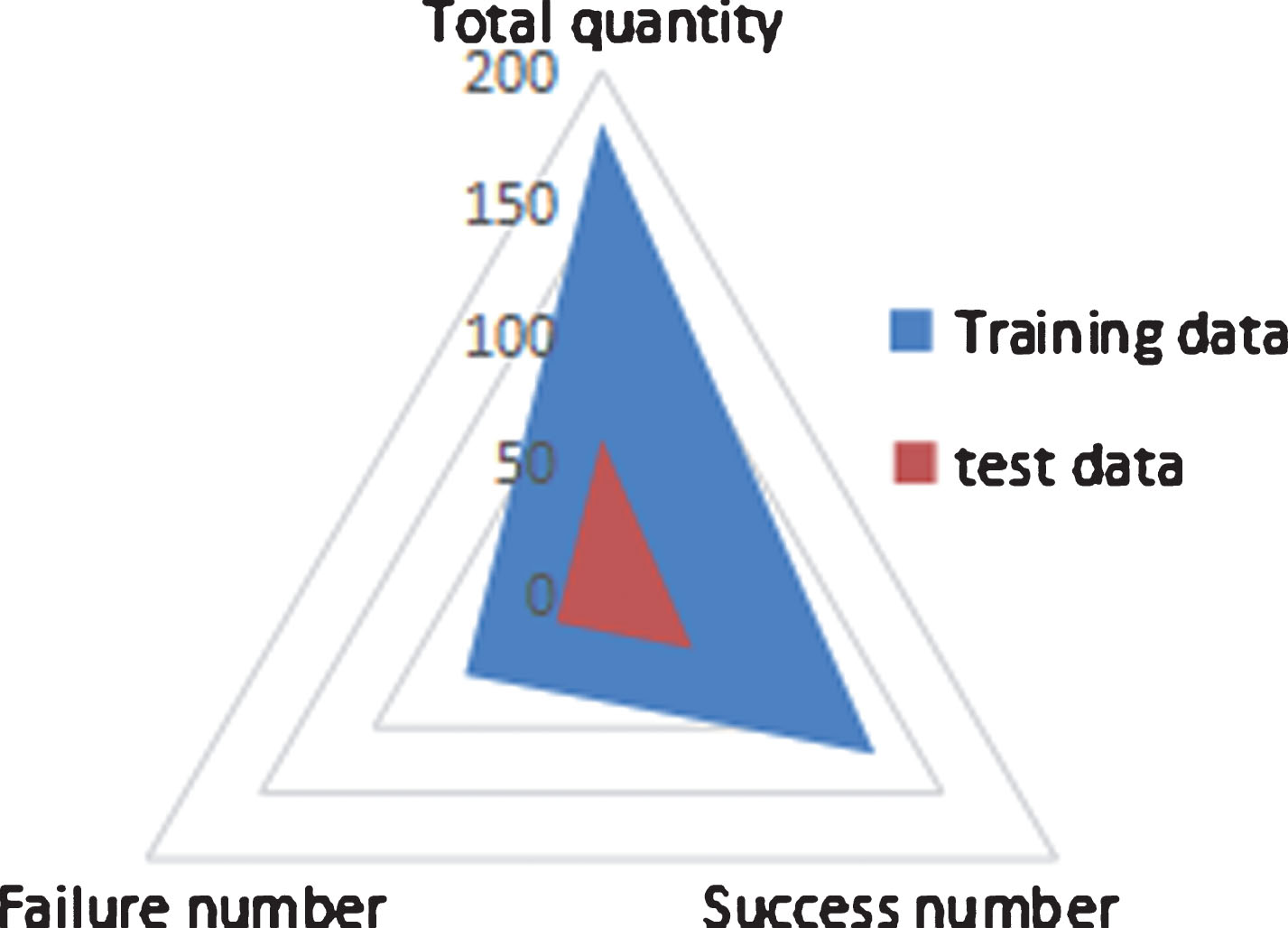
Experimental data statistics.

Fig.5

Comparison image of the accuracy rates of different classification methods.

Judgment and tempo movement start synchronously. In the front hook diagonal movement of the net, only when judging the stability and determining the best hitting point, it is possible to achieve the effect of the front hook diagonal of the net.

Pre-swing acceleration phase (T1 - T2) : It refers to the process from the first maximum point (T1) to the next minimum point (T2) of the hook diagonal track in front of the net before hitting the ball. After the ball is thrown, the racket continues to swing upwards, and the torso swings forward, causing the body to be “bow” before hitting the ball.

Batting stage (T2 - T3) : When the ball descends to the point of hitting, the body quickly slams the ball and stretches the arm and body. When swinging the ball, the wrist that is held by the hand drives the arm to have a whiplash inside the screw. This is the key action of the net front hook diagonal. An action can release all the forces such as the advance of the center of gravity, kicking, turning, swinging, etc. to the ball.

The stage of the fellows (T3 . T4) : After the shot (T3), the holding continues to stretch in the direction of the shot and is guided slightly by the inertial arm, which ends up on the left side of the body. Fellows as an integral part of the complete batting process, smooth stretch of fellows can reduce damage to the joints and muscles. The swing can not only control the power of the shot, but also control the flight path of the ball after hitting the ball, such as: rotation, curvature, and so on.

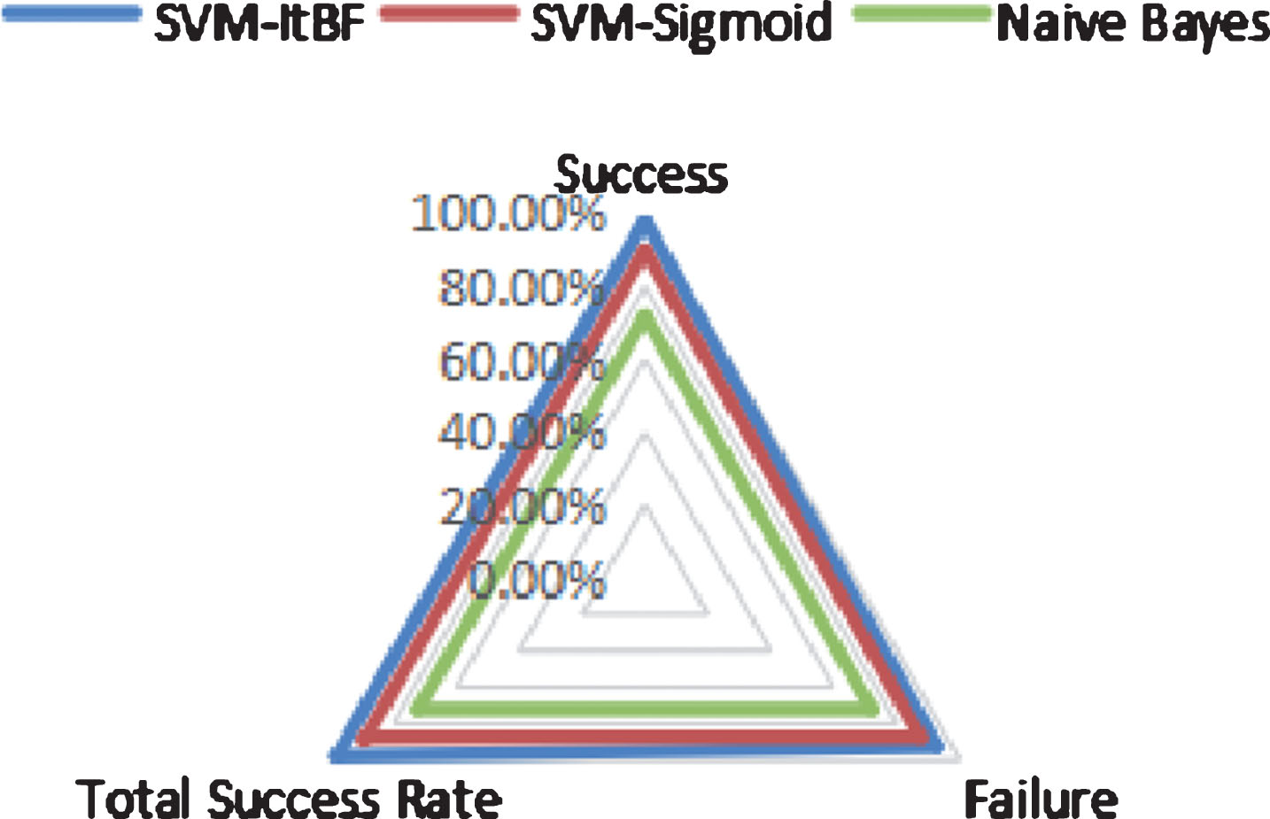
A performance comparison test of each classification method is performed to compare the classification performance of SVM’s Sigmoid kernel function and Radial basis function. With the SVM. Sigmoid and SVM. RBF classifiers, the SVM is trained with training data under the condition of fixed parameters c = 100, a = 4.87. Then, the collected 60 test data is classified and compared with the Naïve Bayes algorithm in terms of accuracy (Accuracy). The results are shown in Table 2.

Table 2

comparison table of accuracy rates of different classification methods

	Success	Failure	Total success rate
SVM-ItBF	98.34%	93%	98%
SVM-Sigmoid	90.13%	88%	89.27%
Naive Bayes	72%	72%	72%

It can be clearly seen from the table that the accuracy of the SVM classification method is higher than that of the naive Bayesian method. Among them, the total accuracy of SVM-Sigmoid method classification is 17.27% higher than that of Naïve Bayesian method, and the accuracy of SVM-RBF is nearly 25% higher than that of Naive Bayesian method. Therefore, this paper chooses the radial basis kernel function as the kernel function of SVM.

6 Analysis and comparison of results

When classifying data using PSO-SVM, the feature data needs to have the same dimension. Therefore, in the four stages of the diagonal front (T0 - T1, T1 - T2, T2 - T3, T3 - T4) , uniform sampling is used, and 30 feature points are collected in each stage. Then, the feature vector and the tag input support vector machine (SVM) are trained. On the machine with the experimental environment of Intel Xeon(R)E5.2620 v3 CPU 2.40GHz and 32.0GB memory, this paper uses MATLAB R2012b and combines LIBSVM to realize the PSO SVM tennis net front hook diagonal model. Moreover, during the training process, the radial basis kernel function is selected as the kernel function of the SVM.

The specific process is: The net front diagonal track data is read into the memory. Then, when the SVM cross-validates the parameters, the optimization is performed by the PSO algorithm to determine the optimal penalty parameter c and the kernel function parameter σ. The default local search ability of the PSO algorithm is cl = 1.5, the default global search ability is c2 = 1.7, the maximum evolution number is maxgen = 100, and the maximum population size is sizepop = 20. The maximum and minimum values of the SVM parameter c are 100 and 0.1, respectively, and the maximum and minimum values of the SVM parameter σ are 1000 and 0.01, respectively. First, 120 sets of net front hook data are used to train the PSO-SVM network. The PSO-SVM model returns the values of the optimal parameters C and g, which are: bestc = 1.347, bestg = 738.8443. The classification accuracy is the fitness, and the fitness curve of the PSO-SVM net front hook diagonal model is shown in Fig. 6.

Fig.6

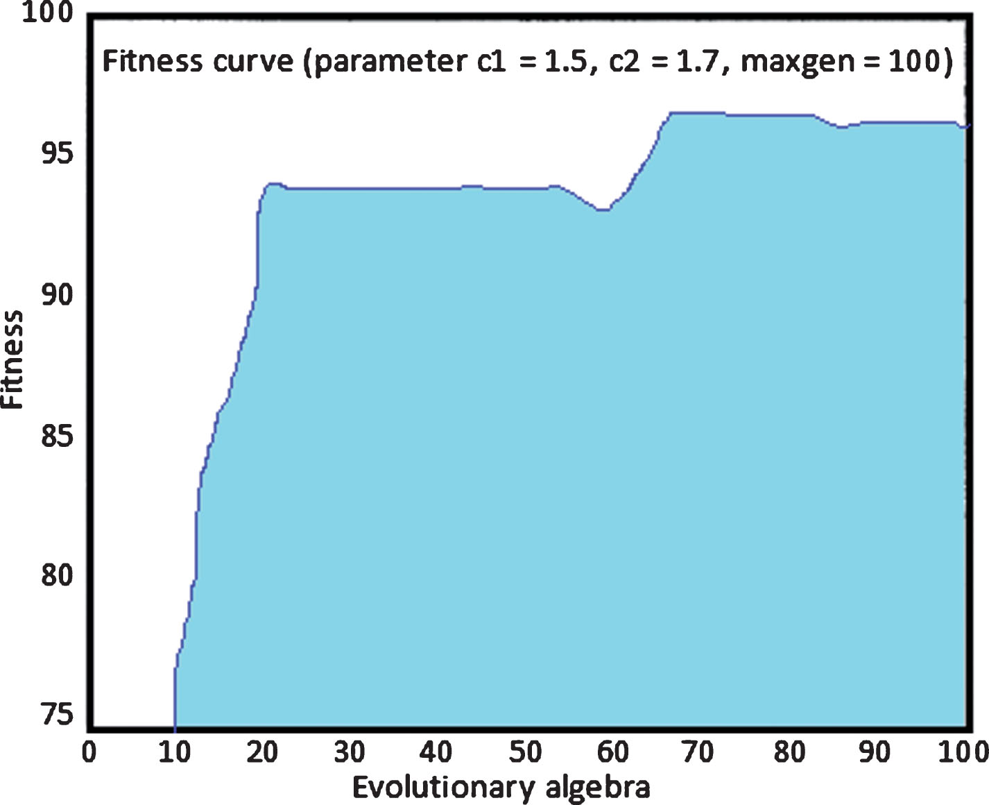
PSO-SVM fitness curve.

It can be seen from Fig. 7 that the accuracy of classification after multiple iterations is 97.5%. Then, this paper uses 60 sets of data as a test set to test this model and test the training effect. The program runs a total of 10 times, and each time 60 error values are generated, and then the error value running time is taken as an absolute average. The results are shown in Table 3.

Fig.7

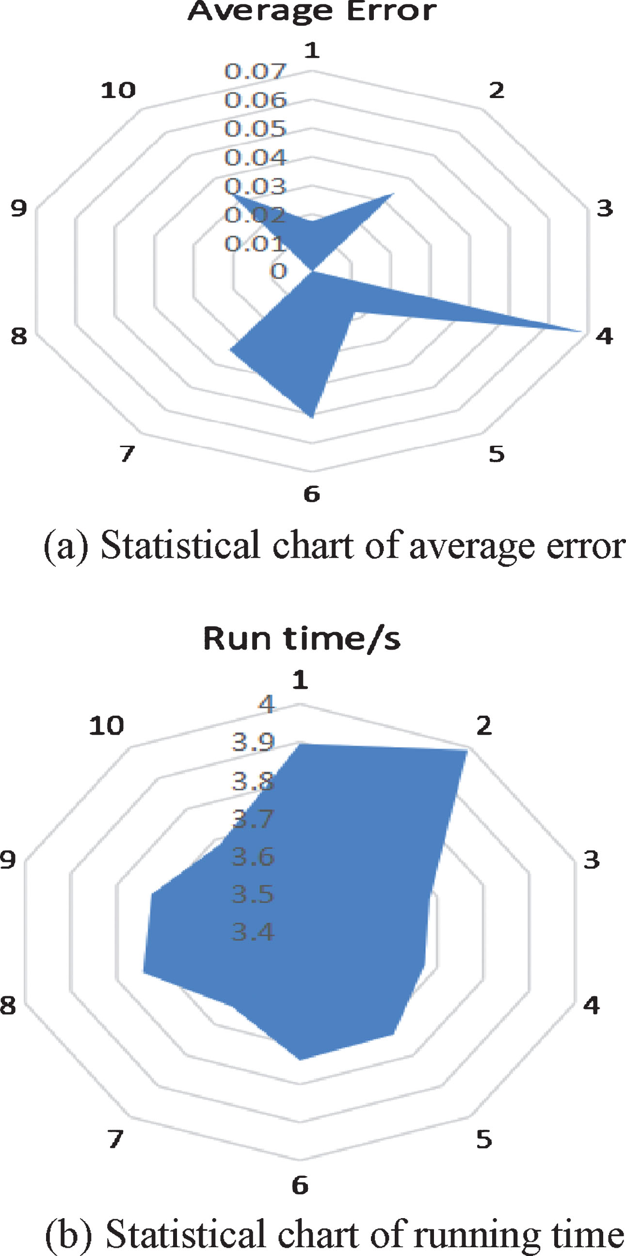
Statistical chart of PSO-SVM simulation results.

Fig.8

Statistics chart of the SVM simulation effect

Table 3

Statistical table of PSO-SVM simulation effect

NO.	Average error	Running time/ s	Average error	Average running time
1	0.01751	3.89577518	0.02575	3.75003018
2	0.03399	3.99121704
3	0	3.68308018
4	0.06901	3.67262465
5	0.01751	3.73123371
6	0.0515	3.7365413
7	0.03399	3.64088417
8	0	3.74208682
9	0	3.72320898
10	0.03399	3.68364771

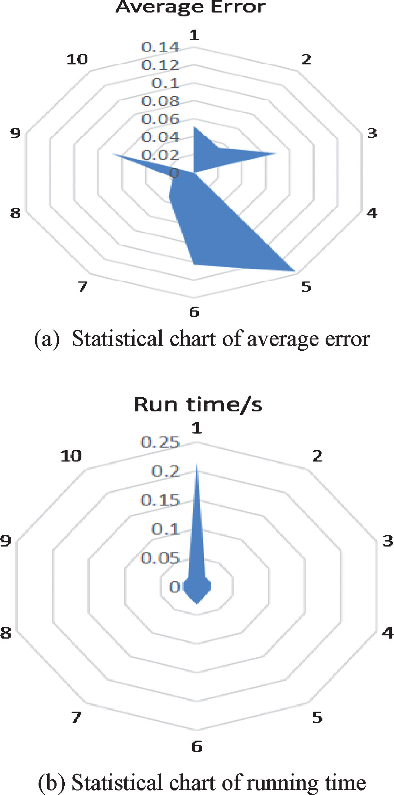
Then the traditional SVM is used to solve the classification problem, and the optimal parameters of the SVM are obtained by the exhaustive method. According to the characteristics of the collected data, the structure of the SVM is the same as that of the PSO-SVM. The SVM net front hook diagonal model is obtained through the training set, and then the training model is tested with the test setThe program runs a total of 10 times, and each time generates 60 error values, and then takes the absolute value of the error value running time. The results are shown in Table 4.

Table 4

Statistical table of SVM simulation effects

NO.	Average Error	Run time/s	Average error	Average running time
1	0.0515	0.2147756	0.05	0.0205568
2	0.03399	0.0196524
3	0.06901	0.01955764
4	0	0.01927336
5	0.13699	0.01928984
6	0.103	0.031724
7	0.03399	0.02023744
8	0.01751	0.01924452
9	0.06901	0.01920332
10	0	0.01922804

By comparison, it can be concluded that the classification error of the PSO-SVM is much smaller than that of the SVM for the classification problem of the hook diagonal trajectory of the net front hook. However, SVM is better than PS0-SVM at runtime. The main reason is that PSO-SVM takes more time to find the optimal parameters. However, if the best parameters c and σ are given directly during the training of the PSO-SVM network (i.e., the time of the optimal parameter search is not considered), the time taken by the two methods is not much different.

7 Conclusion

In order to study the effectiveness of the algorithm in this study, the model case is analyzed and analyzed, and the badminton net front hook diagonal is taken as an example for analysis. In order to establish the PSO-SVM network front diagonal model, firstly, the training set and test set should be extracted from the obtained raw data. Then, this paper conducts certain data analysis and preprocessing, and trains the PSO SVM network with the training set. Finally, this paper uses the obtained model to test and analyze the test data. When classifying data using PSO-SVM, the feature data needs to have the same dimension. Therefore, in the four stages of the diagonal front of the net (T0 - T1, T1 - T2, T2 - T3, T3 - T4) , uniform sampling is used in this paper, and 30 feature points are collected in each stage. The feature vectors and tags are then trained by the input support vector machine (SVM). By comparison, it can be concluded that the classification error of PSO-SVM is much smaller than that of SVM for the classification problem of diagonal trajectory in front of the net. However, SVM is better than PS0-SVM at runtime. The main reason is that PSO-SVM takes more time to find the optimal parameters. However, if the best parameters c and σ are given directly during the training of the PSO-SVM network (i.e., the time of the optimal parameter search is not considered), the time taken by the two methods is not much different. Experiments show that the model can accurately and reliably classify athletes’ detailed actions and achieve expectations. Then, the paper compares and analyzes the model. The results show that this model can provide guidance for dailytraining.

References

Jin

, Jin

S.W.

, Software reliability prediction model based on support vector regression with improved estimation of distribution algorithms, Applied Soft Computing Journal 15(2) (2014), 113–120.

, You

, Yin

, et al., An improved fault-location method for distribution system using wavelets and support vector regression, International Journal of Electrical Power & Energy Systems 55(2) (2014), 467–472.

Ali

, Kamavuako

E.N.

, Scheme

E.J.

, et al., Support vector regression for improved real-time, simultaneous myoelectric control, IEEE Transactions on Neural Systems & Rehabilitation Engineering 22(6) (2014), 1198–1209.

Chan

W.H.

, Mohamad

M.S.

, Deris

, et al., Identification of informative genes and pathways using an improved penalized support vector machine with a weighting scheme, Computers in Biology & Medicine 77(C) (2016), 102–115.

Guo

, Deng

, Jie

, et al., Sensor Multi-fault Diagnosis With Improved Support Vector Machines, IEEE Transactions on Automation Science & Engineering 14(2) (2017), 1053–1063.

Mishra

, Mishra

, SVM-BT-RFE: An improved gene selection framework using Bayesian T-test embedded in support vector machine (recursive feature elimination) algorithm, Karbala International Journal of Modern Science 1(2) (2015), 86–96.

, Zhou

, Li

, et al., Vibrant fault diagnosis for hydro-electric generating unit based on support vector data description improved with fuzzy K nearest neighbor, Proceedings of the Csee 34(32) (2014), 5788–5795.

Ansari

H.R.

, Gholami

, An improved support vector regression model for estimation of saturation pressure of crude oils, Fluid Phase Equilibria 402 (2015), 124–132.

, Chen

, Liu

, et al., Application of support vector machine based on improved grid search in quantitative analysis of gas, Chinese Journal of Sensors & Actuators 28(5) (2015), 774–778.

10.

Miao

, Liu

, Cao

, et al., Malware detection using bilayer behavior abstraction and improved one-class support vector machines, International Journal of Information Security 15(4) (2016), 361–379.

11.

Fattahi

, Application of improved support vector regression model for prediction of deformation modulus of a rock mass, Engineering with Computers 32(4) (2016), 567–580.

12.

Zhi-Jie

, Chun-Yan

Y.U.

, An Improved Support Vector Machines with Balanced Binary Decision Tree forMulti-class Classification, Journal of Chinese Computer Systems 35(5) (2014), 1124–1127.

13.

Dongxiao

, Tiannan

, Bingyi

, Load forecasting by wavelet least squares support vector machine with improved fruit fly optimization algorithm, Journal of Combinatorial Optimization 33(3) (2016), Power 1–22.

14.

, Hua

, Tang

, et al., Modeling of the hot metal silicon content in blast furnace using support vector machine optimized by an improved particle swarm optimizer, Neural Computing and Applications 27(6) (2016), 1451–1461.

15.

A Support. Vector Machine-Based Particle Filter Method for Improved Flooding Classification, IEEE Geoscience and Remote Sensing Letters 12(9) (2015), 1943–1947.

16.

Dharamkar

, Singh

R.R.

, Dharamkar

, et al., Cyber-Attack Classification using Improved Ensemble Technique based on Support Vector Machine and Neural Network, International Journal of Computer Applications 103(11) (2014), 1–7.

17.

Zhang

S.M.

, Li

B.X.

, Wang

B.Y.

, The Application of an Improved Integration Algorithm of Support Vector Machine to the Prediction of Network Security Situation, Applied Mechanics and Materials 513-517 (2014), 2285–2288.

18.

Optimized support vector regression model by improved gravitational search algorithm for flatness pattern recognition, Neural Computing and Applications 26(5) (2015), 1167–1177.

19.

Gangquan

S.I.

, Shuiwang

L.I.

, Jianquan

, et al., Squares Support Vector Machine Parameters Optimization Based on Improved Fruit Fly Optimization Algorithm with Applications, Journal of Xian Jiaotong University 51(6) (2017), Least 14–19.

20.

Zhu

, Wei

, Localization Algorithm in Wireless Sensor Networks Based on Improved Support Vector Machine, Journal of Nanoelectronics & Optoelectronics 12(5) (2016), 452–459.

21.

Fang

, Wu

, Shang

, et al., Failure Prediction of Wind Turbines Using Improved Gray Relation Analysis Based Support Vector Machine Method, Journal of Computational & Theoretical Nanoscience 13(9) (2016), 5887–5895.

22.

, Disaster prediction model based on support vector machine for regression and improved differential evolution, Natural Hazards 85(2) (2016), 1–18.

23.

Yang

, Deng

, Li

, et al., Improved traffic detection with support vector machine based on restricted Boltzmann machine, Soft Computing 21(11) (2015), 1–12.

24.

Kanisha

, Lokesh

, Kumar

P.M.

, et al., Speech recognition with improved support vector machine using dual classifiers and cross fitness validation, Personal & Ubiquitous Computing (3) (2018), 1–9.

25.

Patel

, Sondhi

, Motvani

, et al., Improved Intrusion Detection Technique based on Feature Reduction and Classification using Support Vector Machine and Particle of Swarm Optimization, International Journal of Computer Applications 100(18) (2014), 34–37.