Research on the improvement of the diagnostic effect of machine learning on nuclear magnetic resonance of brain tumors

Abstract

Traditional nuclear magnetic resonance technology has grayscale inhomogeneity in brain tumor detection, which directly affects the formulation of follow-up treatment plans. In order to improve the detection effect of nuclear magnetic resonance on brain tumors, this study uses a convolutional neural network as the basis algorithm to construct an algorithm model suitable for multimodal MRI image recognition. At the same time, combined with the actual case, this paper uses the model to segment and identify brain tumors, and this paper combines the principle of machine learning and collects data for data training to construct a multi-channel deep deconvolution network model. In addition, in order to explore the effectiveness of the algorithm in this study, the performance analysis was carried out by comparative experiment method, and the multi-faceted performance of the model was studied, and the corresponding test result images were obtained. Through experimental comparison, it can be seen that the algorithm model constructed in this study has certain validity, can be applied to practice, and can provide theoretical reference for subsequent related research.

Keywords

Nuclear magnetic resonance brain tumor diagnosis segmentation convolutional neural network

1 Introduction

Nuclear magnetic resonance spectroscopy is mainly used to detect the spectral properties of material molecules based on one-dimensional spectra. However, at present, multidimensional spectroscopy has become the mainstream way. Magnetic resonance multispectral spectroscopy can provide information that classical one-dimensional spectroscopy cannot provide, and plays an important role in structural identification, functional analysis, and other chemical biological studies. Especially in modern medical research, biological macromolecules such as human immune proteins need to be detected by magnetic resonance technology. Moreover, magnetic resonance imaging is widely used in clinical diagnosis and is an important tool for assisting medical diagnosis and treatment [1]. However, both multi-dimensional magnetic resonance spectroscopy and magnetic resonance imaging have the disadvantage of excessive data acquisition time. At the same time, with the expansion of the sampling dimension, the time multiplication law increases and often exceeds the acceptable range. How to provide the same amount of information with less sampling time has become an important hot topic in the field of magnetic resonance research [2].

Brain tumor image segmentation is a very important step in the diagnosis and treatment of brain tumors. By segmenting the tumor in an MRI image, the surgeon can locate the tumor and obtain the size of the tumor, then develop relevant treatment and rehabilitation strategies. In recent years, with the enrichment of material life and the development of science and technology and the improvement of related technology diagnostic techniques, computer-aided diagnosis research on brain tumors has gradually grown [3].

Brain tumor segmentation is a technique for dividing different tumor tissues from normal tissues such as gray matter, white matter and cerebrospinal fluid, such as active tumor tissue, edema tissue, and necrotic tumor tissue. Due to the high clinical relevance and challenge of tumor segmentation itself, brain tumor segmentation has received extensive attention in the past 20 years [4]. According to the degree of human intervention, image segmentation of brain tumors can be divided into three categories: manual segmentation based on manual, semi-automatic segmentation based on manual initialization, and fully automatic segmentation without human intervention. Manual segmentation is a tedious, tedious, time-consuming task [5], and different segmenters have different tendency to segment. However, manual segmentation is a relatively professional and relatively accurate segmentation method for obtaining tumor information from images. In the semi-automatic and automatic segmentation methods, the results of manual segmentation are often used as the object of comparison, which is called Ground Truth, and provides a qualitative and quantitative analysis basis. For semi-automatic segmentation, its segmentation results are relatively dependent on human initialization [6].

Nuclear magnetic resonance testing is an effective way to diagnose brain tumors. However, in practical applications, the use of nuclear magnetic resonance and technology has been difficult to meet the needs of patients. Therefore, it is necessary to combine advanced computer processing technology with nuclear magnetic resonance detection methods, and on this basis, effectively improve the detection effect. This study combines machine learning and nuclear magnetic resonance to improve the detection of nuclear magnetic resonance technology through machine learning.

2 Related work

In 1939, physicist Rabi discovered that the hydrogen molecular beam absorbs electromagnetic waves of a specific frequency in the magnetic field to produce deflection [7], and accurately measures the magnetic properties of atoms and molecules by resonance method, thus obtaining the 1944 Nobel Prize in Physics. In 1946, Purcell [8] of Havard University and Bloch [9] of Stanford University independently discovered nuclear magnetic resonance phenomena from paraffin and liquid water [10], and nuclear magnetic resonance was gradually established as a discipline. In the 1950s, the chemical shift phenomenon discovered by Proctor et al. [11] and the spin coupling phenomenon discovered by Hahnet al. [12] made NMR a good way to study molecular structure. In 1966, Ernst and Anderson implemented a pulsed Fourier transform NMR experiment [13], which improved the sensitivity of NMR and achieved a revolutionary development. In 1976, Ernst [14] and others first realized the two-dimensional nuclear magnetic resonance experiment and established the theoretical basis for the two-dimensional NMR spectrum [15]. The two-dimensional spectrum is an important milestone in the nuclear magnetic resonance spectrum, and Ernst also won the 1991 Nobel Prize in Chemistry. In addition, with the development of the manufacturing process, the excitation magnetic field frequency of the nuclear magnetic resonance spectrometer is further improved, which means that the resolution of the obtained nuclear magnetic resonance spectrum is increasing.

Nuclear magnetic resonance is mainly caused by the spin motion of the nucleus. According to the difference of the spin quantum number, it can be divided into a magnetic nucleus and a non-magnetic nucleus. The former can produce nuclear magnetic resonance phenomenon, and at least one of its proton number or neutron number is an odd number, so the spin quantum number is not 0; The latter proton and neutron numbers are even, and the spin quantum number is 0, which does not produce nuclear magnetic resonance. In the absence of an applied magnetic field, the orientation of the magnetic core in the material, that is, the orientation of the axis of the spin motion of the magnetic core, is irregular. However, after the substance is placed in an external magnetic field, the orientation of the magnetic core changes, which is consistent with or opposite to the magnetic field. When the magnetic nucleus is stabilized in an applied magnetic field, the magnetic nucleus is excited by a certain frequency of radio frequency electromagnetic waves. At this time, the magnetic nucleus resonates, and an offset occurs in the radio frequency direction, and the spin axis is offset with respect to the direction of the magnetic field, which is called precession. When the RF pulse is over, the spin axis of the magnetic core will gradually return to the state of the applied magnetic field. The time required for recovery is called the relaxation time. If the gyro returns to the spin axis and remains vertical, the relaxation time has two parts [15].

Today, many physics, chemistry, and biology research institutes use NMR as an important method of research. Moreover, NMR equipment is also evolving rapidly, and the frequency of NMR spectrometers has increased, from the use of permanent magnets to the use of superconductors, and the improvement of NMR spectrometers has driven the advancement of scientific research. In addition, NMR is also widely used in daily life. The most important thing is that in medical treatment, magnetic resonance imaging (Magnetic Resonance Imaging) has become an indispensable information for doctors to diagnose diseases [16].

In recent years, ZhiliangWei, JianYang, Youhe Chen et al. [17] proposed a Fourier transform on the basis of K space, and the resulting space is called “trans K space”, and the signal is corrected in the trans-K space. The corrected trans-K-space spectrum is then subjected to inverse Fourier transform back to K-space, and the accuracy and spectral width of the obtained two-dimensional spectrum are significantly improved.

The introduction of NMR/MRI analysis into algorithms such as machine learning/pattern recognition and other computer fields is a trend in recent years. In 2013, Nature [17] proposed a pattern recognition algorithm to design separate “fingerprints” for different tissues and substances, and to identify the collected spectrum based on these “fingerprints” through an intelligent classifier. The “fingerprint” in the article is also the feature used in the machine learning classifier. After collecting these signals, the classifier is trained, and the corresponding signals are manually labeled as fat, protein, and the like. Moreover, the trained classifier is used for the classification of the newly acquired signals. On the other hand, in MRI, digital image processing and machine learning are more widely used. Because of the extensive combination of MRI and medical, biological [18], etc., machine learning has been used, such as PET/MRI tissue signal attenuation correction [19], brain tumor classification [20], neuroimaging analysis [21] and so on. At the same time, machine learning has achieved many achievements in the field of magnetic resonance imaging.

3 Theoretical basis of the algorithm

3.1 Solving the sparse representation model

The sparse representation model can often be solved in two steps:First, the feature vector is fixed, and each input training sample is solved for its corresponding sparse coefficient a_i. Secondly, the sparse coefficient a_i is fixed, and the base feature vector φ_i is updated one by one to make it better represent the input sample vector space. The first step is the process of sparse coding, and the second step is generally called dictionary update in the sparse representation model.

The algorithms for solving sparse coding can be divided into two major categories, one is the relaxation algorithm, and the other is the greedy algorithm.

The relaxation algorithm refers to a convex sparseness loss function that is relatively easier to handle and is chosen to replace the non-convex |₀ norm by using the characteristicthat the optimization of the convex function can be solved.

The original sparse representation model is the loss function, which takes the |₀ norm as the sparsity. The |₀ norm is closest to the defined sparsity in a specific physical sense, and the |₀ norm is used to solve the model to obtain the most satisfactory result. However, unfortunately, the mathematical nature of the |₀ norm is very bad. The most significant point is that the |₀ norm is a function that cannot be divisible everywhere. Therefore, it is impossible to find its optimal solution by means of derivation. The traditional way to solve the |₀ norm optimization problem is: It assumes that the |₀ norm of the sparse coefficient a_i is L, L = 1, 2, 3, ⋯ , k. When L = 1, there are a total of k combinations. Then, whether there is a vector group that satisfies the sparse representation loss function is calculated. If it exists, the solution is successful, otherwise L is increased by 1;When L = 2, there are a total of k (k - 1)/ - 2 combinations. Then, whether there is a vector group that conforms to the loss function is calculated. If it exists, the calculation ends, otherwise L continues to increase by one, and so on. It can be found that the above algorithm is an NP-hard problem. When k is a large value, it is impossible to exhaust all possible combinations. Therefore, it is considered to replace the original |₀ norm with a more easily processed |₁ norm to convert the original combinatorial optimization problem into a linear programming problem. The most classic representation of the relaxation algorithm is the Basic Pursuit.

By using |₁ norm instead of the original |₀ norm, the purpose of convenient and fast solution can be achieved. However, under what preconditions, the solution obtained by |₁ norm and |₀ norm will be equivalent? In 2006, Chinese mathematician Tao Zhexuan proved that under the RIP condition, the |₀ norm optimization problem and the |₁ norm optimization problem will get the same solution. The so-called RIP conditions are described as follows: The constants μ, N satisfy [22]: $\begin{matrix} (1 - μ N) {∥ a ∥}_{2}^{2} ⩽ {∥ a θ ∥}_{2}^{2} ⩽ \\ μ N {∥ a ∥}_{2}^{2} \forall {∥ a ∥}_{0} ⩽ N \end{matrix}$ (1)

Therefore, under the condition that the RIP theorem is satisfied, the |₁ norm can be used as the sparsity loss function to solve the satisfactory solution, which plays a crucial role in the promotion of the sparse representation model.

The main idea of the greedy algorithm is to first determine the position of the non-zero element in the sparse coefficient a, and then calculate the value of the non-zero element by stepwise adjustment. Compared with the relaxation algorithm, the greedy algorithm greatly reduces the time complexity. Matching Pursuit and Orthogonal Matching Pursuit are two classic greedy algorithms.

The basic idea of the matching pursuit algorithm is [23]:

θ_i ∈ D, i = 1, 2, ⋯ , k, and D is called a dictionary consisting of “supercomplete” basis vectors. First, a base that is closest to the input signal x is selected from the dictionary, and then a set of sparse coefficients is obtained to construct a sparse representation. At this point, the residual between the original input signal x and the sparse representation can be found, and then the resulting residual is replaced by the obtained residual. Next, a base that best matches the residual signal is selected from the dictionary, a set of sparse coefficients is obtained, and a new sparse representation is constructed to obtain a new residual. This iteration is repeated until the final residual is less than the initially set threshold.

3.2 Group sparse representation classifiers that combine |₁, |₂ norm

A key point of the classifier method based on sparse representation is the target neuroimaging feature vector to be represented from the training samples. It assumes that there are N training samples:

{s₁, ⋯ s_n, ⋯ s_N } is represented by an X matrix, respectively, X = [X₁, · sX_l, · sX_c] ∈ R^M×N. These training samples belong to different categories of C numbers (the problem of the two classifications is studied, so C is equal to 2), and N = N₁ + N_l + N_c X_l ∈ R^M×N_l. It includes N_l number of training samples belonging to category 1. All feature vectors in this article are represented as column vectors, unless otherwise stated. Moreover, the symbol ∥ · ∥ ₁ represents the standard |₁ norm symbol of the vector, and ∥ · ∥ ₂ represents the standard European norm of the vector, also known as the |₂ norm. Then, a sparse representation of the test sample is obtained from the non-parametric dictionary by an |₁ norm minimization optimization method. However, the classification method for test samples is to evaluate which type of dictionary corresponds to a smaller reconstruction error. A test sample y is given, then the classifier based on sparse representation attempts to solve such an optimization problem with minimization of |₁ norm: $\hat{a} = arg min_{a} {∥ Xa - y ∥}_{2}^{2} + λ {∥ a ∥}_{1}$ (2)

The above-mentioned |₁ norm minimization problem can be solved by the sparse coding solution of the |₁ norm regular term mentioned above, such as relaxation algorithm and greedy algorithm. Ideally, the resulting sparseness coefficient $\hat{a}$ should be closely related to a training sample from a class, so the test sample y can be easily classified directly into this class. However, noise and errors that occur during the modeling process will cause non-zero conditions for sparse coefficients corresponding to other classes. Therefore, different from the previous classification using the sparse coefficient to distinguish the test sample, the classifier based on the sparse representation classifies by evaluating, judging the sparseness coefficient $\overset{⌢}{a} l$ and the corresponding training samples X_l belonging to the class 1 can be used to reconstruct test samples for classification. Such a classification method can make better use of the subspace structure of each class corresponding to the training sample. Therefore, for a test sample y, its final classification is as follows [25]: $Label (y) = arg min_{l} {∥ X_{l} {\hat{a}}_{l} - y ∥}_{2}$ (3)

The above |₁ norm-based sparse representation classifier assumes that non-zero values in the sparse coefficients are completely random. In other words, it is assumed that the noise appearing in the training sample is white noise similar to the standard. However, the sparse coefficients corresponding to the data samples usually show the essential and inherent structural information in the form of groups. Therefore, the introduction of the inherent packet structure information into the sparse representation model is a reasonable strategy to improve the accuracy of the sparse representation classifier. In addition, for data samples, sharing the basis vectors of the same class dictionary, in other words, the more average the sparse coefficients corresponding to the same type of base vector, the easier it is to improve the resolution of a sparse representation classifier. In order to take into account the inherent packet structure information of the sparse signal, a group sparse representation method is proposed, which includes the class grouping information of the training samples into the sparse representation model. In the group sparse representation method, the |₁ norm regular term is replaced by the |₂ norm regular term, and its mathematical expression is as follows [25]: $\hat{a} = arg min_{a} {∥ Xa - y ∥}_{2}^{2} + λ \sum_{i = 1}^{c} ω_{i} {∥ a_{G_{i}} ∥}_{2}$ (4)

Among them, the symbol a_{G
_i} represents the sparse coefficient corresponding to the category G group i. After the grouping information is added, the test data can be approximated as a linear combination of training samples within each group.

Although the sparse representation model based on the |₁ norm regularization introduces sparsity into the representation coefficients, it uses a test object-dependent approach when selecting training sample data, so it is limited in the use of packet structure information. Therefore, this paper decides to integrate the |₁ and |₂ norm regular terms, and make full use of the grouping structure information of the training samples under the premise of ensuring the sparseness of sparse coefficients, so that the sparse representation classifier model can be extended to some extent in the classification problem: $\begin{matrix} \hat{a} = arg min_{a} {∥ Xa - y ∥}_{2}^{2} + λ_{1} {∥ a ∥}_{1} \\ + λ_{2} \sum_{i = 1}^{c} ω_{i} {∥ a_{G_{i}} ∥}_{2} \end{matrix}$ (5)

In this paper, the classification problem of mild cognitive dysfunction transition (MCI-C) and mild cognitive dysfunction non-transformer (MCI-C) is taken as an example. Then, all training samples X will be divided into two groups according to the category: one is the data set corresponding to the MCI-C group and the other is the data set X₂ corresponding to the MCI-NC group. The symbol a_{G
₁} represents the coefficient corresponding to the MCI-C group in the sparse coefficient, and the symbol a_{G
₂} represents the coefficient corresponding to the MCI-NC group in the sparse coefficient. The group sparse representation classifier scheme of the fusion |₁, |₂ norm proposed in this paper can make full use of the sparse characteristics brought by the |₁ norm and the packet differentiation information brought by the group |₂ norm to get better classification results.

For the optimization of (5), the Moreau-Yosida regularization method can be used to solve it. Moreover, a penalty factor for sparse grouping can be introduced in the solution process. By adjusting the sizes of the parameters λ₁ and λ₂, it can be used to weigh the weights of the norm |₁ and the group |₂ norm.

Finally, by solving the Equation (5), the sparse coefficient corresponding to each test sample can be obtained. Then, the test samples can be classified according to the reconstruction error remainder of the minimum formula (3). Finally, the test samples will be assigned to the category corresponding to the minimum reconstruction error. For test objects with multiple time point image data, the classification decision can be determined by the sum of the reconstruction errors of all time point data.

4 Deep deconvolution network model

Inspired by U-Net’s use of deconvolution network models in cell detection and segmentation problems, based on DeconvNet and SegNet, in this paper, the multi-mode MRI image data is used to introduce the deconvolution network model from the semantic segmentation problem into the brain tumor segmentation based on MRI images, and the tissue structure of the tumor is described in the MRI slices data. The corresponding basic network model structure is shown in Fig. 2.

Fig.1

Schematic diagram of the matching pursuit algorithm.

Fig.2

Schematic diagram of the deconvolution network structure model.

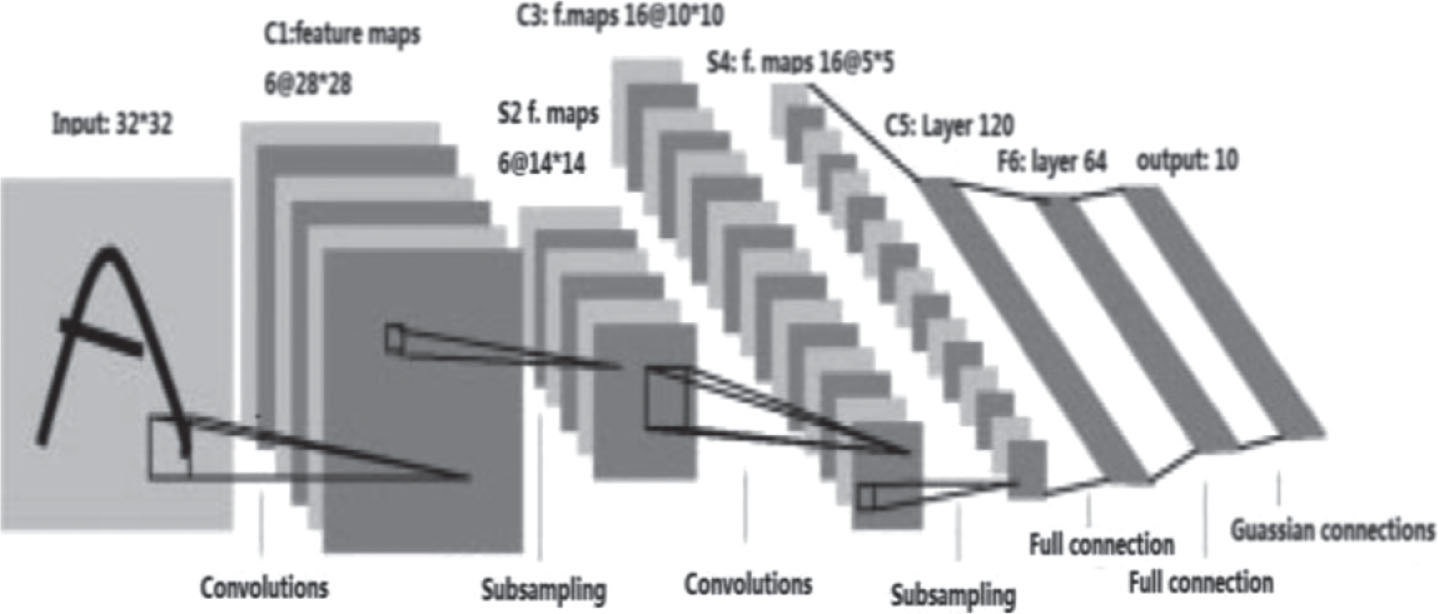
As depicted in Fig. 2, the network trained in this paper consists of two parts: convolution and deconvolution, which can also be said to be the coding part and the decoding part. The convolution network is used as a feature extractor to extract corresponding feature descriptions from the input MRI slices imageand the deconvolution network is used as a shape generator to generate a segmentation target from the extracted feature map. Finally, the softmax network is used to generate the final segmentation result, and the corresponding segmentation result is obtained by predicting the tumor class to which each pixel belongs. In this paper, the convolutional network of VGG-16 is used as the convolution part, including 13 convolutional layers, and some convolutional layers are connected by connecting the activation layer or the pooling layer. Then, the 2 fully connected layers enhance the mapping of the specific class by converting the fully connected layer into a convolutional layer similar to the FCN. The deconvolution layer is a mirrored result of the convolutional layer (such as the mirror structure described in Fig. 2), and the segmentation result is finally obtained by transposition convolution and multiple de-pooling operations. At the same time, it should be noted that the process of full-connection convolution is not detailed here.

It can be seen from the input of each layer of the network that a multi-channel target image to be segmented is input and extracted through the feature of the full convolution network. Then, using the cascaded deconvolution network, the extracted features can be restored to the original pixel space through the learned convolution kernel. Finally, through softmax, the reconstructed feature map is predicted and classified to obtain a probability map corresponding to the original pixel space, that is, the prediction label required for the split task. MRI brain tumor image segmentation is taken as an example, and the final classification number is set to k (1 ⩽ k ⩽ 4), and a training set { (x¹, y¹) , (x², y²) , . . . , (x^m, y^m)}is given, yⁱ∈ { 1, 2, . . . , k }. Now, an input test data x is given, and the probability of each class is estimated by calculating the corresponding probability value p (y = j|x) for each class. Finally, a k-dimensional normalized vector is output: $h_{θ} (x^{i}) = [\begin{matrix} p (y = 1 | x^{i}; θ) \\ p (y = 2 | x^{i}; θ) \\ . . . \\ p (y = k | x^{i}; θ) \end{matrix}] = \frac{1}{\sum_{j}^{k} e^{θ_{j}^{T} x^{i}}} [\begin{matrix} e^{θ_{1}^{T} x^{i}} \\ e^{θ_{2}^{T} x^{i}} \\ . . . \\ e^{θ_{k}^{T} x^{i}} \end{matrix}]$ (5)

Among them, θ₁, . . . , θ_k ∈ Rⁿ⁺¹ is the model parameter, and each element of the final output vector corresponds to a probability estimate of the corresponding one of the tumor structure categories and the element sum is 1. In this way, a softmax probability estimate for each pixel in the original image is obtained. Then, it is mapped to each category to be divided, and finally the segmentation result is output.

5 Test analysis

On the basis of theoretical research, through the experimental exploration and data analysis, the multi-modal brain tumor image segmentation problem using deep deconvolution network is elaborated in detail: Firstly, the DeconvNet self-pre-training deconvolution network model is used, and then the quality of pre-training model is compared with the quality of pre-training mode of the direct training and the fine-tuning of vgg-16.

5.1 Analysis of neural network training results

The training of neural networks has always been a cumbersome and time-consuming problem, and a complete training is usually at least thirty hours (for this article). In order to get better pre-training results, this paper uses three methods for training. First: using the first stage of DeconvNet training methods; second: using the vgg-16 network model trained in imagenet as a pre-training model; third: direct training. In the pre-training with DeconvNet, in order to obtain an effective pre-training model, a preliminary attempt was made to explore. The more important one is the adjustment of the learning rate: A part of the slices samples are selected, and the exploration training with fewer iterations is performed on the basis of adjusting the learning rate, so as to determine a learning rate which can converge better and faster, and to obtain a better pre-training model.

As shown in Fig. 3, the results of the loss change of the training process at the learning rates of 0.01, 0.001, 0.00001, and 0.000001 are listed separately. It can be seen that at LR = 0.000001, the loss slowly falls. It can be foreseen that the final convergence needs to take a long time and more iterations. Therefore, the LR is increased by an order of magnitude and adjusted to LR = 0.00001, and after entering more than 9000 iterations, there is a tendency for convergence to begin. Then, by an increase of 2–3 orders of magnitude, it can be found that in a shorter time, a better training result than before can be obtained. However, there have been some unexpected situations. For this reason, after several trial trainings and tests, finally, at LR = 0.0001, the pre-training results as shown in Fig. 4 were obtained.

Fig.3

Full convolutional network structure.

Fig.4

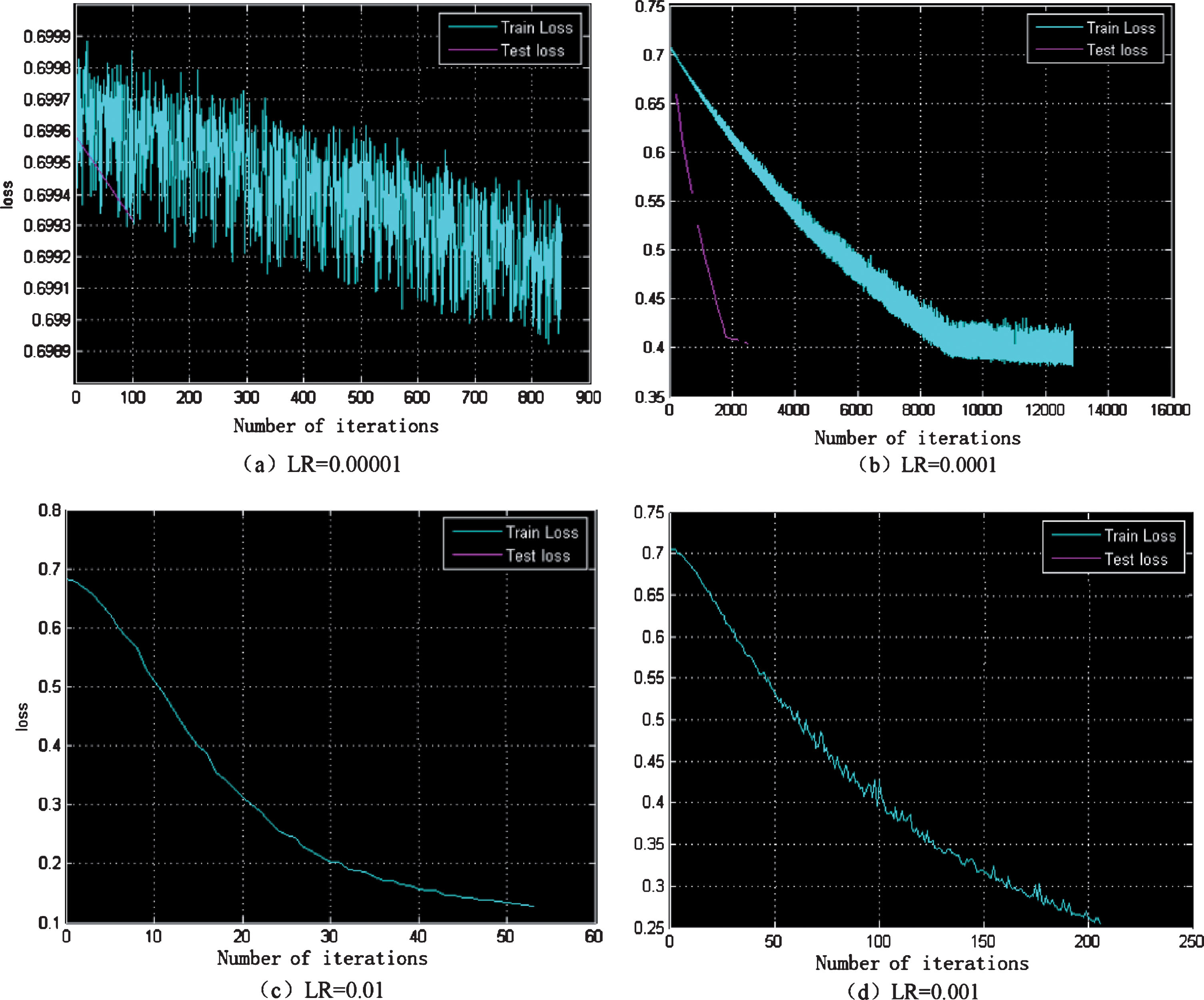
Schematic diagram of the loss change of the pre-training model at different learning rates, (a) LR = 0.00001, (b) LR = 0.0001, (c) LR = 0.01, (d) LR = 0.001.

As mentioned above, this paper uses a deep deconvolution model of multi-path to establish sub-models for each type of tumor structure. Next, the corresponding training and test results will be analyzed from the segmentation accuracy rate in the training process of each sub-network model. Compared with the results obtained by the fine tuning of Vgg16, the results obtained by the DeconvNet model pre-trained by the tumor sample have a small amplitude of convergence during the convergence process. At the same time, the average accuracy rate is relatively high. Of course, only the accuracy rate does not describe the quality of the training process. Therefore, the loss of the training process also needs to be concerned. As shown in Fig. 5, the loss changes curves of three tumor structure (whole, active, core) in the process of using DeconvNet pre-training and Vgg16 pre-training are listed separately. It can be seen that the loss of using Vgg16 has a more beautiful convergence curve than the loss of DeconvNet. The DeconvNet’s loss maintains a small amplitude and enters the state of convergence earlier.

Fig.5

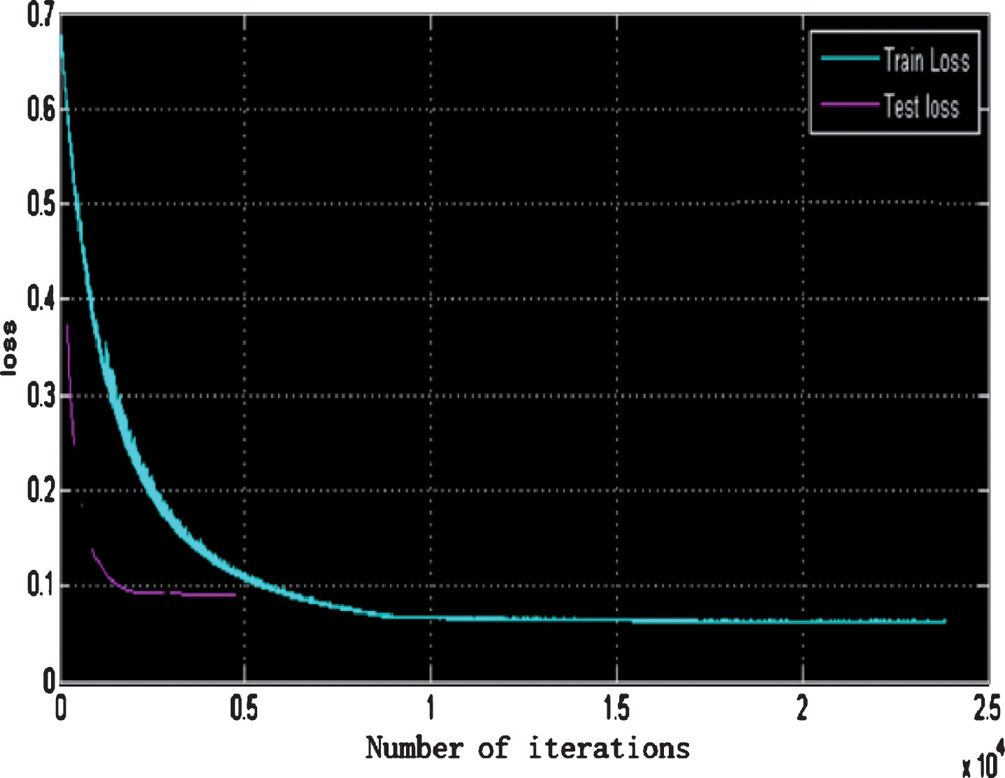
Schematic diagram of loss decline trained and verified by pre-trained models.

Fig.6

Loss changes in the tumor structure pre-training model.

Fig.7

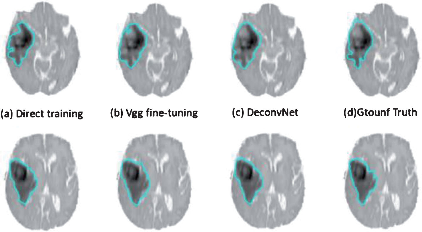
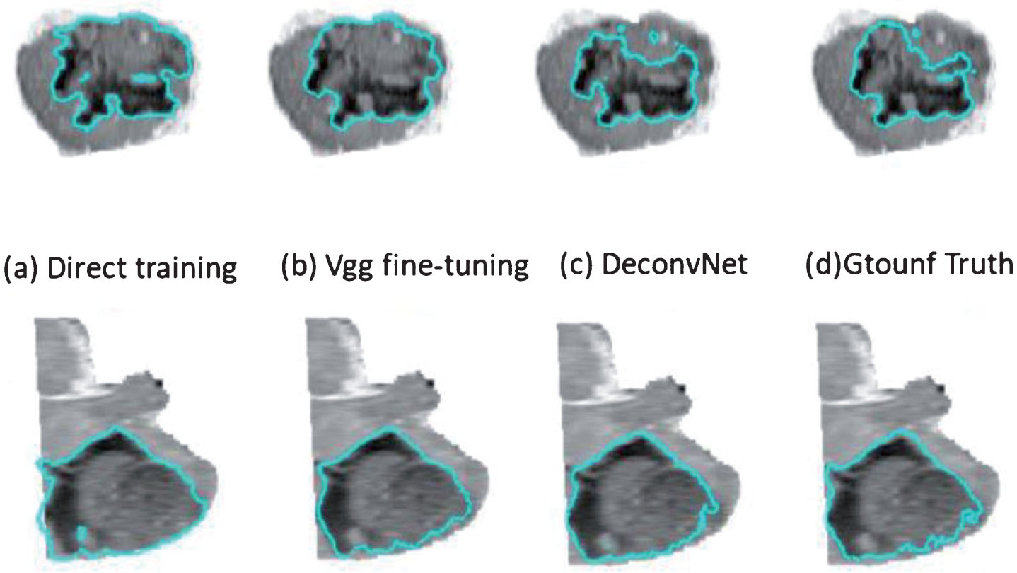
Example of Whole segmentation results of three different training modes in the axial direction.

Fig.8

Example of Whole segmentation results of three different training modes in the sagittal direction.

Fig.9

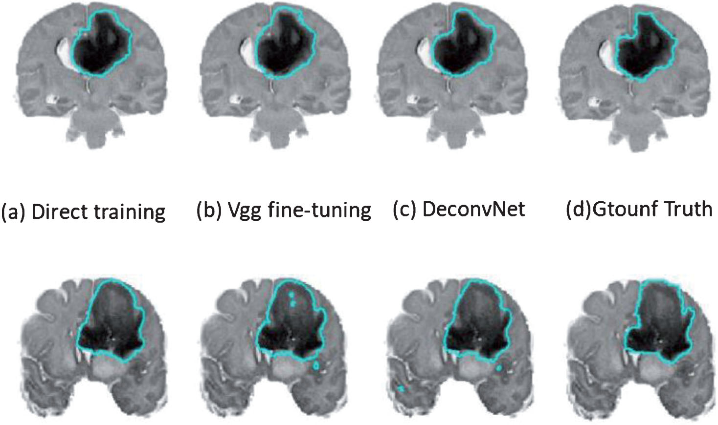
Example of Whole segmentation results of three different training methods in the coronal direction.

It can be seen that the accuracy of training using the Vgg and DeconvNet pre-training models is higher than the result of direct training. Moreover, the classification accuracy of different categories of training predictions also has a large difference. The specific reasons will be discussed in the following sections. This training prediction accuracy also has a certain guiding effect on the determination of the later segmentation model. Based on this, it can be predicted that the pre-training model obtained by Vgg and DeconvNet can better adapt to the task of brain tumor segmentation. Of course, the specific results still need to be determined in the process of model testing for the segmentation description and quantitative analysis of each structure.

6 Analysis of results

In order to fully illustrate the segmentation effectiveness of the multi-path hybrid deep deconvolution neural network, in the following three aspects of segmentation of the whole tumor, tumor core area and tumor active tissue, the results of the segmentation test results of three different training methods are taken as an example, and the ground truth results are compared in the three axial slices of interest. Meanwhile, in order to describe the final segmentation result, an edema structure, an active tissue structure, and a necrotic tissue structure in tumor tissues are also exemplified. Of course, quantitative results analysis is also necessary.

It can be clearly found that the results of using DeconvNet fine-tuning are better than the other two methods. Although the details are not as intuitive as direct training, the segmentation of the entire tumor is most similar to ground truth. After obtaining the segmentation result of the entire tumor, if the segmentation result of the tumor core region and the active tissue region is obtained, the structure of the edema region and the tumor necrotic tissue of the tumor can be obtained by the weighted region subtraction method and a certain post-treatment. In order to achieve such a goal, a fine segmentation of the tumor structure is obtained, and the effectiveness of the deep deconvolution network structure of the multipath subnetwork is described in the process of segmenting the tissue structure of the tumor. From the outside to the inside, it is roughly divided into edema area and tumor nucleus. Moreover, in the structure of the tumor nucleus, it can be further divided into an active tissue region and a necrotic region.

From the above results, it can be seen that the use of a deep deconvolution network model combined with multimodal MRI images is very effective for segmentation of brain tumor images. Of course, these structures are separate examples of the division of a structure and organization, and the detailed results of the segmentation cannot be described as a whole. To this end, the method based on multi-channel deep deconvolution neural network designed in this paper is quantitatively analyzed. Through the final segmentation results of the three training methods adopted in this paper,it can be seen that the use of model fine-tuning is more reliable than direct training.

7 Conclusion

This study combines machine learning with nuclear magnetic resonance and enhances the detection of nuclear magnetic resonance technology through machine learning. 本 At the same time, based on DeconvNet and SegNet, this paper introduces the deconvolution network model from the semantic segmentation problem into the brain tumor segmentation based on MRI images through multi-modal MRI image data and multi-channel specific segmentation network training. In addition, in order to fully explain the segmentation effectiveness of the multi-path hybrid deep deconvolution neural network, in the three aspects of segmentation of the whole tumor, tumor core area and tumor active tissue, this paper takes the segmentation test results of three different training methods as an example and compares the test results with the ground truth results in the three axial slices of interest. The results show that the use of deep deconvolution neural network methods is a very effective solution scheme for brain tumor segmentation. Moreover, the use of a deep deconvolution network model combined with multimodal MRI images is very effective in segmenting brain tumor images.

References

Mason

, Al-Qaisieh

, Bownes

, et al., Multi-parametric MRI-guided focal tumor boost using HDR prostate brachytherapy: A feasibility study, Brachytherapy 13(2) (2014), 137–145.

Yue

, Bin

, Fei

, et al., In vivo tomographic imaging with fluorescence and MRI using tumor-targeted dual-labelednanoparticles, International Journal of Nanomedicine 9(9) (2014), 33–41.

Njeh

, Sallemi

, Ayed

I.B.

, et al., 3D multimodal MRI brain glioma tumor and edema segmentation: A graph cut distribution matching approach, Computerized Medical Imaging & Graphics the Official Journal of the Computerized Medical Imaging Society 40 (2015), 108–119.

Heerkens

H.D.

, Van Vulpen

, Van d B

C.A.T.

, et al., MRI-based tumor motion characterization and gating schemes for radiation therapy of pancreatic cancer, Radiotherapy and Oncology 111(2) (2014), 252–257.

Park

J.A.

, Lee

Y.J.

, Ko

I.O.

, et al., Improved tumor-targeting MRI contrast agents: Gd(DOTA) conjugates of a cycloalkane-based RGD peptide, Biochemical and Biophysical Research Communications 455(3–4) (2014).

Alimohamadi

, Sanjari

, Mortazavi

, et al., Predictive value of diffusion-weighted MRI for tumor consistency and resection rate of nonfunctional pituitary macroadenomas, Acta Neurochirurgica 156(12) (2014), 2245.

Grossmann

, Gutman

D.A.

, Dunn

W.D.

, et al., Imaging-genomics reveals driving pathways of MRI derived volumetric tumor phenotype features in Glioblastoma, BMC Cancer, 16(1) (2016), 611.

Burbach

J.P.M.

, Kleijnen

J.P.J.

, Reerink

, et al. Inter-observer agreement of MRI-based tumor delineation for preoperative radiotherapy boost in locally advanced rectal cancer, Radiotherapy and Oncology, 118(2) (2016), 399–407.

MRI Tumor Volume Reduction Rate vs Tumor. Regression Grade in the pre-operative re-staging of locally advanced rectal cancer after chemo-radiotherapy, European Journal of Radiology 84(12) (2015), S0720048X15300814.

10.

Ramanathan

R.K.

, Korn

, Raghunand

, et al., Correlation Between Ferumoxytol Uptake in Tumor Lesions by MRI and Response to Nanoliposomal Irinotecan in Patients With Advanced Solid Tumors: A Pilot Study, Clinical Cancer Research 23(14) (2017), 3638–3648.

11.

Barnes

S.L.

, Sorace

A.G.

, Loveless

M.E.

, et al., Correlation of tumor characteristics derived from DCE-MRI and DW-MRI with histology in murine models of breast cancer, NMR in. Biomedicine 28(10) (2015), 1345–1356.

12.

Recurrence-free survival in breast cancer is associated with MRI tumor enhancement dynamics quantified using computer algorithms, European Journal of Radiology 84(11) (2015), S0720048X15300553.

13.

Lopes

, Jayaswal

D. A.

Methodical Approach for Detection and 3-D Reconstruction of Brain Tumor in MRI, International Journal of Computer Applications 118(17) (2015), 37–43.

14.

Suero

G.A.

, Abreu , Praveen Raju

, Aristizábal , Orlando , et al., In Vivo Mn-Enhanced MRI for Early Tumor Detection and Growth Rate Analysis in a Mouse Medulloblastoma Model, Neoplasia 16(12) (2014), 993–1006.

15.

Kim

H.R.

, You

D.G.

, Park

S.J.

, et al., MRI monitoring of tumor-selective anticancer drug delivery with stable thermosensitive liposomes triggered by high-intensity focused ultrasound, Molecular Pharmaceutics (2016), acs.molpharmaceut.6b00013.

16.

Luhach

, Idiyatullin

, Lynch

C.C.

, et al., Rapid ex vivo imaging of PAIII prostate to bone tumor with SWIFT-MRI, Magnetic Resonance in Medicine 72(3) (2014), 858–863.

17.

Usman

, Rajpoot

. Brain tumor classification from multi-modality MRI using wavelets and machine learning, Pattern Analysis and Applications 20(3) (2017), 871–881.

18.

Xin-Xing

, Zhao-Xia

Yang

, He-Yue

Liang

, et al., Whole^-tumor MRI histogram analyses of hepatocellular carcinoma: Correlations with Ki^-67 labeling index, Journal of Magnetic Resonance Imaging JMRI 46(2) (2016).

19.

Kragha

K.O.

Malignant Peripheral Nerve Sheath Tumor: MRI and CT Findings, Case Reports in Radiology 2015 (2015), 1–7.

20.

Canellas

, Lo

, Bhowmik

, et al., Pancreatic neuroendocrine tumor: Correlations between MRI features, tumor biology, and clinical outcome after surgery, Journal of Magnetic Resonance Imaging 47(2) (2018).

21.

Chen

, Liu

, Chen

, et al., Targeted tumor MRI with gadobutrol-loaded anti-HER2 immunoliposomes,, ActaRadiologica (2016), 0284185116664225.

22.

Johnson

D.R.

, Diehn

F.E.

, Giannini

, et al., Genetically defined oligodendroglioma is characterized by indistinct tumor borders at MRI, AJNR American Journal of Neuroradiology 38(4) (2017).

23.

Neubauer

, Li

, Verena

Müller

, et al., Diagnostic Value of Diffusion-Weighted MRI for Tumor Characterization, Differentiation and Monitoring in Pediatric Patients with NeuroblasticTumors, RöFo - Fortschritte auf demGebiet der Röntgenstrahlen und der bildgebendenVerfahren 189(07) (2017), 640–650.

24.

Smith

, Taplin

A.L.

, Syed

. et al., Correlation between intraoperative ultrasound and postoperative MRI in pediatrictumor surgery, Journal of Neurosurgery: Pediatrics (2016), 1–7.

25.

Rajendran

, Liang

, Tang

Y.A. M

, et al., Optimization of arterial spin labeling MRI for quantitative tumor perfusion in a mouse xenograft model, Nmr in Biomedicine 28(8) (2015), 988–997.