Self labeling online sequential extreme learning machine and it’s application

Abstract

In the field of big data machine learning, the data volume is large, but the labeled data is few. Due to this, it may lead to that the distribution of labeled data (source domain) is not similar to that of unlabeled data (target domain). In traditional machine learning field, this problem is a kind of transfer learning problems. To address this problem, a self labeling online sequential extreme learning machine is presented, which is called SLOSELM. Firstly, an ELM classifier is trained on the labeled training dataset of the source domain. Secondly, the unlabelled dataset of the target domain is classified by the ELM classifier. In the third step, the high confident samples are selected and the OSELM is employed to update the original ELM classifier. Tested on the real-world image dataset and the daily activity dataset, the results show that our algorithm performs well.

Keywords

Extreme learning machine activity recognition transfer learning big data pervasive computing

1 Introduction

In the traditional supervised learning, it is typically assumed that the unlabeled test data comes from the same distribution as the labeled training data. However, generally the two data sets have different distributions, and in recent years, machine learning researchers have investigated methods to handle mismatch between the training and test domains, with the goal of building a classifier on the labeled data in the old domain(source domain) to perform well on the test data in the new domain(target domain).

To address this problem, many algorithms are presented under the framework of transfer learning, and it is a common scenario in speech processing applications and activity recognition problems. Self-labeling approaches include self-training, co-training, and Maximum Likelihood Linear Regression (MLLR). Self-training is based on the Expectation Maximization (EM) algorithm. The basic EM algorithm [1] aims to maximize the log likelihood log(p(x|θ)) of observed data x. The computation of log(p(x|θ)) depends on some “hidden” or missing variables z. In the transfer learning setting, we want to maximize the log likelihood log(p(x|θ)) both on the observations of labeled data (xi, yi) ∈ L and unlabeled data xi ∈ U, with the labels of L as hidden variables. And the relative importance of the labeled and unlabeled data should be traded off. Co-training [2] is a transfer learning method based on the idea of multi-view learning. Two different classifiers are trained based on different “views” (i.e., feature representations). For each classifier, it is used to label new instances from the unlabeled data set and the confident samples are used as another classifier’s training data to train a new one on the next round. This process is repeated till the model converged. MLLR is used for speaker adaptation in speech recognition and was first proposed by [3] and [4]. MLLR adapts a Gaussian mixture HMM to new unlabeled speaker data. It assumes that the Gaussian mixture components in the two domains have the corresponding relationship via linear transformation of means and variances in each Gaussian. Therefore, the model can automatically label the target domain data and the old model can be updated. All the above self labeling approaches need to merge the original training data and the predicted samples to retrain a new model. However, with the training data increasing, the training time will be increased. Therefore, an online sequential learning algorithm is promising.

Sequential learning algorithms have also become popular for feedforward networks. These include resource allocation network (RAN) and its extensions. However, all the sequential learning algorithms process data one by one only and cannot process data chunk by chunk basis. An online sequential extreme learning machine(OSELM) [5] is introduced. OSELM can handle the training data in a sequential manner. At any time, only the newly arrived single or chunk of data (instead of the entire past data) are seen and learned. After the learning procedure, the current chunk of data is discarded immediately. Based on these advantages, OSELM is a promising method and will be employed in our SLOSELM.

In this paper, to address the transfer learning and power efficient problem in big data fields, a self labeling online sequential extreme learning machine is presented, which is abbreviated SLOSELM. First, an ELM classifier is trained on the labeled training data set of the source domain. Second, the unlabeled data set of the target domain is classified by the ELM classifier. In the third step, the high confident samples are selected and the OSELM is employed to update the original ELM classifier.

The rest of the paper is organized as follows. In Section 2, SLOSELM is presented in detail. In Section 3, experiments on SLOSELM is given. Section 4 concludes the paper.

2 Self labeling online sequential extreme learning machine

SLOSELM (Self Labeling Online Sequential Extreme Learning Machine) consists of three steps: First, on the labeled samples from source domain, an initial ELM classifier is trained. The ELM model’s parameters, such as randomly selected input weight vector α, bias vector b, activated function G(a, b, x) and the number of hidden nodes L, the hidden layer output matrix H and the output weight β, are reserved. Second, for a chunk of unlabeled samples from target domain, they are classified by the ELM classifier and from the initial classification results, the high confident samples are chosen out. In the third step, based on the high confident samples, OSELM is employed to update the current ELM model. With the unlabeled samples coming chunk by chunk, Step 2 to Step 3 is repeated.

Place the file in any of the directories where MS Word looks for templates. These directories are defined within MS Word under Tools/Options/File Locations.

2.1 Brief of extreme learning machine

Figure 1 shows the network structure of ELM(Extreme Learning Machine) [6 –9], it is a SLFNs (Sigle layer feedforward networks). SLFNs have been studied for several decades. Most of the existing methods for training SLFNs, such as the famous back-propagation algorithm and the Levenberg-Marquardt algorithm, employ gradient methods to optimize the weights in the network. Some existing works also use forward selection or backward elimination approaches to construct network dynamically during the training process. However, neither the gradient based methods nor the grow/prune methods guarantee a global optimal solution. Although various methods, such as the generic and evolutionary algorithms, have been proposed to handle the local minimum problem, they basically introduce high computational cost. One of the most successful algorithms for training SLFNs is the support vector machines (SVMs), which is a maximal margin classifier derived under the framework of structural risk minimization (SRM). The dual problem of SVMs is a quadratic programming and can be solved conveniently. Due to its simplicity and stable generalization performance, SVMs have been widely studied and applied to various domains. ELM is a recent neural network algorithm, which is known to achieve good performance in complex problems as well as reduce the computation time compared with other machine learning algorithms [10 –13]. The ELM algorithm does not train the input weights or the biases of neurons, but it acquires the output weights by using the norm least-squares solution and Moore-Penrose in verse of a general linear system [14]. By finding the node giving the maximum output value, we decide the final result.

Fig.1

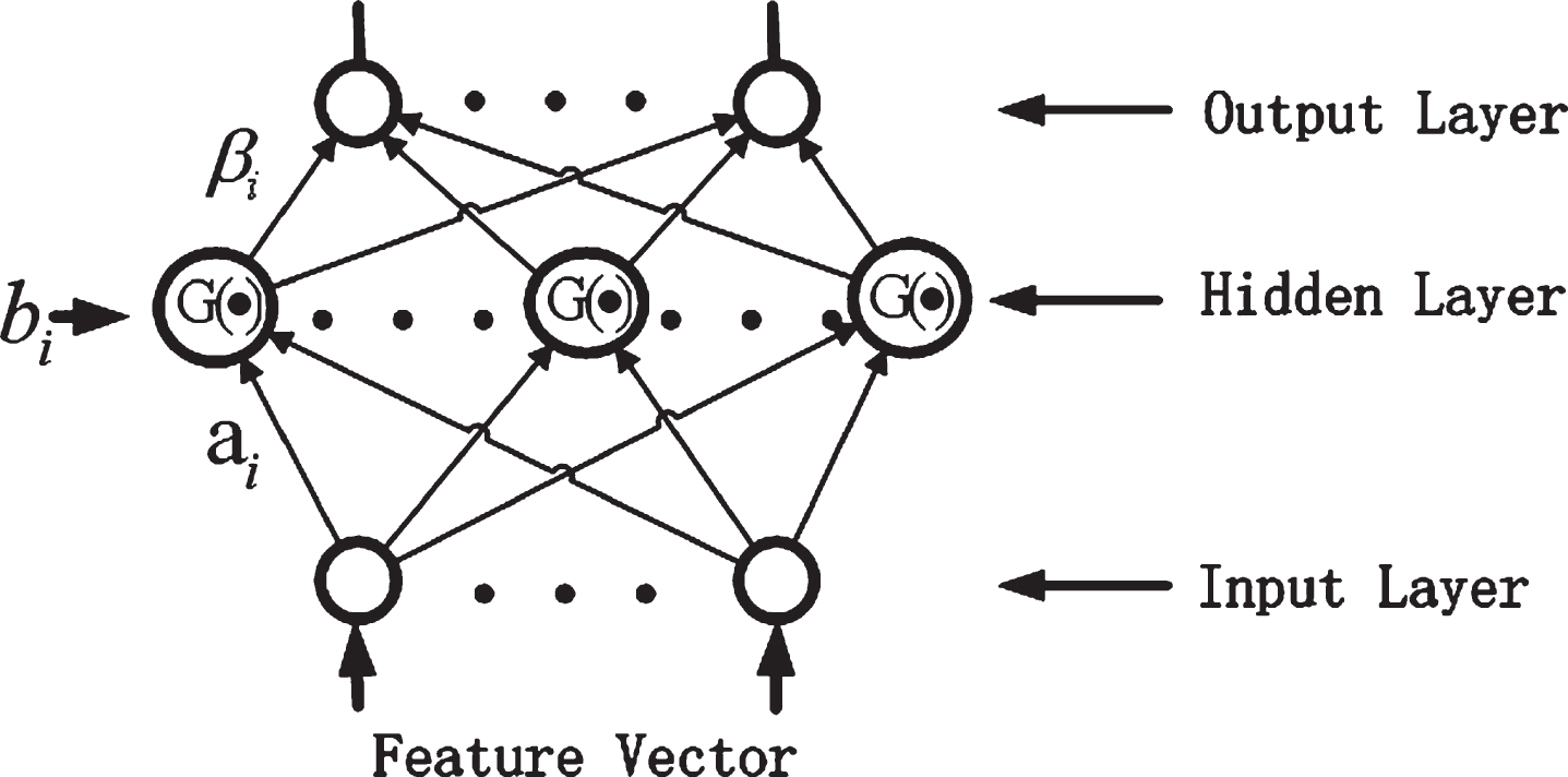
The network structure of ELM.

The learning phase for the ELM with a single hidden layer can be summarized as Algorithm 1.

Algorithm 1

the ELM Algorithm

Require: Given a traning set ℵ = {(x_i, t_i) |x_iRⁿ, t_i ∈ R^m,

i = 1, 2, . . . , N} activation function G(x), and hidden node

number

\tilde{N}

Ensure.

the weight β.

1. Randomly assign input weight α₁ and bi as b_i,

i = 1, 2, . . ., \tilde{N}

2. Calculate the hidden layer output matrix H:

H = {(\begin{matrix} G (α_{1} . x_{1} + b_{1}) & \dots & G (α_{\bar{N}} . x_{1} + b_{\bar{N}}) \\ ⋮ & \dots & ⋮ \\ G (α_{\bar{N}} . x_{N} + b_{1}) & \dots & G (α_{\bar{N}} . x_{N} + b_{\bar{N}}) \end{matrix})}_{N \times \bar{N}}

3. Calculate the output weight β = H † T, where H is the

Moore-Penrose generalized invrse of matrix H,

T = [t₁, …, t_N] ′.

4. RETURN β.

2.2 Self labeling the unlabeled instances

When the ELM classifier is learned and used to classify a new instance x, the outputs can be calculated as follows: ${TY}_{1 \times m} = [G (a_{1}, b_{1}, x), . . ., G (a_{L}, b_{L}, x)]_{1 \times L} β_{L \times m}$ (1)

Where m is the number of output nodes, which equals the number of classes in classification problem, and TY is a vector including m values. Then, the classifier selects the maximum value of |1 – TY| and assigns its corresponding index, j, as the class label of the test instance. $j = \underset{j \in [1, m]}{arg min | 1 - {TY}_{j} |}$ (2)

Furthermore, a confidence can be assigned to the instance, which is applied to show to what extent it approximates the assigned class label. The confidence can be calculated by the following steps:

1) Calculate the distance between each component of TY and 1.

$D = | 1 = TY |$ (3)

2) Calculate the reciprocal of each component in D, it can be written as following:

$D_{Inverse} = \frac{1}{D}$ (4)

3) Calculate the proportion of the maximum value in the DInverse as the confidence of the sample x:

$confidence = \frac{Max (D_{Inverse})}{\sum D_{Inverse}}$ (5)

According to the confidence, the instance can be evaluated. If the confidence is less than a threshold,, the corresponding instance can be seen as a noise and discarded. Otherwise, the instance and its assigned label can be reserved as a sample.

When sufficient enough, the new samples can be used to update the model. We can merge the previous training data and the new samples to rebuild a new classifier. However, in real applications, the training data may arrive chunk-by-chunk, hence, the batch ELM algorithm has to be modified for this case so as to make it online sequential.

2.3 Online sequential extreme learning machine

The ELM described above assumes that all the training data is available for training. However, in real applications, the training data may arrive chunk-by-chunk or one-by-one (a special case of chunk). Therefore, the batch ELM algorithm has to be modified so as to make it online sequential.

Step1. Given a chunk of initial training set: $ℵ_{0} = (x_{i}, t_{i})_{i = 1}^{N_{0}}$ , assign random input weight ai and bias bi, select the activated function G(a, b, x) and hidden node number L. The hidden layer output matrix H0 can be calculated: $H_{0} = {[\begin{matrix} G (a_{1}, b_{1}, x_{1}) & \dots & G (a_{L}, b_{L}, x_{1}) \\ ⋮ & \dots & ⋮ \\ G (a_{1}, b_{1}, x_{N_{0}}) & \dots & G (a_{L}, b_{L}, x_{N_{0}}) \end{matrix}]}_{N_{0} \times L}$ (6)

Then the output weight $β_{0} = K_{0}^{- 1} H_{0}^{T} T_{0}$ , where $K_{0} = H_{0}^{T} H_{0}$ . And T₀ = [t₁, t₂, . . . , t_{N
₀}] ^T.

Step2. Suppose now that we are given another chunk of data $ℵ_{1} = {(x_{i}, t_{i})}_{i = N_{0} + 1}^{N_{0} + N_{1}}$ , then using the ai, bi, G, L in Step1, the H1 can be calculated. $H_{1} = {[\begin{matrix} G (a_{1}, b_{1}, x_{N_{0} + 1}) & \dots & G (a_{L}, b_{L}, x_{N_{0} + N_{1}}) \\ ⋮ & \dots & ⋮ \\ G (a_{1}, b_{1}, x_{N_{0} + N_{1}}) & \dots & G (a_{L}, b_{L}, x_{N_{0} + N_{1}}) \end{matrix}]}_{N_{1} \times L}$ (7)

Furthermore, we can get the following results: $K_{1} = {[\begin{matrix} H_{0} \\ H_{1} \end{matrix}]}^{T} [\begin{matrix} H_{0} \\ H_{1} \end{matrix}] = [H_{0}^{T} H_{1}^{T}] [\begin{matrix} H_{0} \\ H_{1} \end{matrix}] = K_{0} + H_{1}^{T} H_{1}$ (8)

Therefore, the solution is $\begin{matrix} β_{1} K_{1}^{- 1} = {[\begin{matrix} H_{0} \\ H_{1} \end{matrix}]}^{T} [\begin{matrix} T_{0} \\ T_{1} \end{matrix}] = K_{1}^{- 1} \\ (K_{1} β_{0} - H_{1}^{T} H_{1} β_{0} + H_{1}^{T} T_{1}) β_{0} + K_{1}^{- 1} H_{1}^{T} (T_{1} = H_{1} β_{0}) \end{matrix}$ (9)

As can be seen in formula (9), β1 is a function of β0, K1, H1 and T1, and not a function of the data set ℵ₀.

2.4 The Algorithm of SLOSELM

The algorithm of SLOSELM can be described in Algorithm 2.

Algorithm 2
Self Labeling Online Sequential Extreme Learning Machine

Require:

The labeled source domain $D_{src} = {(x_{src,}^{(i)} t_{src,}^{(i)})}_{i = 1}^{No},$ where $t_{src}^{(i)}$ is

the label of $x_{src}^{(i)}$ the labeled source domain $D_{src} = {(x_{src}^{(i)})}_{i = 1}^{No},$

does not have any labeled samples. Only the instance number

of D_src is larger than a threshold,η, the self labeling algorithm

is applied.

Ensure:

the weight β

1: Assign random input weught, select the activated

function G (a, b, x)

2: calculate

$H_{0} = {(\begin{matrix} G (a_{1}, b_{1}, x_{1}) & \dots & G (a_{\bar{N}}, b_{\bar{N}}, x_{1}) \\ ⋮ & \dots & ⋮ \\ G (a_{1}, b_{1}, x_{NO}) & \dots & G (a_{\bar{N}}, b_{\bar{N}}, x_{N 0}) \end{matrix})}_{N \times \bar{N}}$ . Set k = 0

3: While |D_tar|η do

4: for each x in $D_{tar} = {x_{tar}^{ι}}_{i = 1}^{N_{2}} do$

5: ${TY}_{i \times m} = [G (a_{1}, b_{1}, x), . . ., G (a_{N}, b_{N}, x_{No})] 1 \times \bar{N} . β_{\bar{N} \times m}$

6: j = arm minTY_i,j is the predicted label of x.

7: MinValue = arg min TY_j ;

8: TY = TY - min Value ;

9: ifconfidence = arm min TY_j/_TY∑_∈TYTY_i

10: confidence > 0.5 then

11: HConfset = HConfset+ x ;

12: D_tar = D_tar - x ;

13: end if;

14: end for

15: k = k+ 1 ;

16: According to high confident dataset, Hconset, calculate

$H_{ko} = {(\begin{matrix} (G (a_{1} . x_{| Hconset |}^{1} + b_{1}) & \dots & G (a_{\bar{N}} . x_{| Hconset |}^{1} + b_{\bar{N}}) \\ ⋮ & \dots & ⋮ \\ G (a_{1} . x_{| Hconset |}^{N} + b_{1}) & \dots & G (a_{\bar{N}} . x_{| Hconset |}^{N} + b_{\bar{N}}) \end{matrix})}_{N \times \bar{N}}$

17: $K_{ko} = K_{ko - 1} + H_{ko}^{T}$

18: $β_{ko} = β_{ko - 1} + K_{ko}^{1} H_{ko}^{T} (T_{ko} - H_{ko β - 1})$

19: end While

20: RETURN β

3 Experiments

In this section, the SLOSELM was tested on two image datasets and an activity dataset. Both two image datasets used in the experiment come from UCI machine learning repository (http://archive.ics.uci.edu/ml). The data in the activity dataset is collected from accelerometer based activity recognition field, in which the model trained on the data from some specific locations can not well distinguish the data from other locations.

3.1 Data collection

Both two image datasets used in the experiment come from UCI machine learning repository, with one named image segments and the other satellite images.

In our activity recognition experiments, Nokia N95 8GB mobile phones are used to collect the accelerometer data. An activity dataset is built from the data collected from these devices. In this database, there are 4 participants and 5 activities. The sliding window with 50% overlapping method is used to extract the features. The sampling frequency of N95 accelerometer sensor has been reduced to approximately 32 Hz by calling the Nokia Accelerometers plug-in API. Our chosen window size is two seconds and the overlapping time is one second. Thus a complete action can be included in the window. Feature extraction on windows with 50% overlapping has demonstrated successful in previous work [18].

3.2 Feature extraction

Image segments includes 2310 subimages, which are extracted from 7 outdoor images, and each subimage has a size of 3 pixels×3 pixels. From each subimage, 19 attributes are extracted, based on which the subimage is classified as 1 of the 7 original images. Satellite images are scenes captured by landsat multispectral scanner with 4 channels, and therefore 4 images are obtained in each frame. One frame is selected, and the region of interest is delineated (82 pixels×100 pixels) so that the subimages (3 pixels×3 pixels) are extracted. The purpose is to classify the central pixels into any of the 6 categories based on 36 attributes of the subimages (red soil, cotton crop, gray soil, damp gray soil, soil with vegetation stubble, and very damp gray soil). Basic information of image segments database and satellite images database is shown in Table 1.

Table 1
The information of image datasets

Name of dataset Number of attributes Number of categories of samples Number of samples

Image segment 19 7 2310

Satellite image 36 6 6435

Name of dataset	Number of attributes	Number of categories of samples	Number of samples
Image segment	19	7	2310
Satellite image	36	6	6435

For triaxial accelerometer, the output voltages can be mapped into acceleration along three axes, ax, ay, az. As ax, ay, az are the orthogonal decompositions of real acceleration, the magnitude of synthesized acceleration can be expressed as: $a = \sqrt{a_{x}^{2} +} a_{y}^{2} + a_{z}^{2}$ , where a is the magnitude of real acceleration, but has no directional information. Therefore, the acceleration magnitude based activity recognition model is orientation independent. Based on the acceleration magnitude series, 17 statistic features [15] are extracted from a sliding window of 256 samples with 50% overlapping between consecutive windows. These features are mean, standard deviation, energy, mean-crossing rate, maximum value, minimum value, first quartile, second quartile, third quartile, four amplitude statistic features and four shape statistic features of the power spectral density (PSD) [16]. In addition, based on FFT transformation of the acceleration magnitude series, all frequency components from 1Hz to 128Hz are extracted and added into the feature vector, totally 145 features. To eliminate the scaling effects among different features, all the features are normalized using the z-score normalization algorithm. The number of samples of every activity are listed in Table 2.

Table 2

The information of daily activity samples

Activity name	Label	Number of samples
Staying Still	1	4520
Downstairs	2	4293
Walking	3	4327
Running	4	4245
Upstairs	5	4369

3.3 Performance evaluation of ELM

The performance of SLOSELM is evaluated on the dataset described above. All the simulations have been done on the MATLAB2009a environment running on an ordinary PC with 2.6GHz CPU. The source code of ELM and OSELM are download from Professor Huang’s page3. The sigmoid function is used as the activation function. In the following experiments, 100 is selected as the optimal number of hidden nodes.

3.3.1 Image validation

In this section, the experiments aim to test the ELM algorithms’s ability to recognize image data. For each class, the data are randomly divided into two parts, 10% and 90%, which are called training data and test data, respectively. The training data are used to train a classifier to test the test data. Above process is repeated for 10 times, the average experiment results are listed in Table 3.

Table 3
Result of recognition experiment for ELM on image dataset

Name Dataset of training data Dataset of test data Average accuracy

Satellite image 10% 90% 58.02%

Image segment 10% 90% 57.05%

Name	Dataset of training data	Dataset of test data	Average accuracy
Satellite image	10%	90%	58.02%
Image segment	10%	90%	57.05%

From Table 3, we can see that the average accuracy is about 60%, and it can be called a weak classifier. The reason is that the training data is too few to describe the distribution of test data.

3.3.2 Cross location validation

In this section, the experiments aim to test the ELM algorithms’s ability to recognize activity data from different locations. Three locations, Hand, Chest Pocket and Trousers Pocket, are presented as A, B and C. The datasets of these locations are represented as DataA, DataB and DataC, respectively. Each dataset is randomly divided into two equal parts, which are represented as DataA1 and DataA2, DataB1 and DataB2, and DataC1 and DataC2. Without loss of generality, we first assume that A and B are known locations and C is a new one. TrainAB, which equals DataA1 U DataB1, is used to train an ELM model. Then, the ELM model is tested on TestAB, which equals DataA2 U DataB2, and DataC respectively. The process is repeated three times and each location is made as the new location in turn. The experiment results are listed in Table 4.

Table 4
ELM Recognition results on the known and unknown locations

TrainData from known loc Acc on known loc TestData from unknown loc Acc on unknown loc

TrainAB TestAB 81.07% DataC 67.85%

TrainBC TestBC 88.41% DataA 62.02%

TrainAC TestAC 74.53% DataB 64.08%

Mean Accuracy 81.34% 64.65%

TrainData	from known loc	Acc on known loc	TestData from unknown loc	Acc on unknown loc
TrainAB	TestAB	81.07%	DataC	67.85%
TrainBC	TestBC	88.41%	DataA	62.02%
TrainAC	TestAC	74.53%	DataB	64.08%
Mean	Accuracy	81.34%		64.65%

As can be seen from Table 4, while the test data come from the distribution as training data, the recognition accuracy is high. However, while they come from the different distribution, the accuracy is poor. Therefore, the cross location activity recognition problem should be under the transfer learning framework.

3.4 Performance evaluation of SLOSELM

3.4.1 Image validation

In this section, the experiments aim to test the SLOSELM algorithms’s transfer learning ability to image dataset. The data in image dataset is randomly divided into 10 equal parts. The first part is used to train the initial ELM classifier. The 2–9 parts are used one by one to update the classifier. The 10th part is used to test the classifier. This process is repeated 10 times, the average performance is listed it following table. From Table 5, we can see that the weak classifier can become a strong classifier by using SLOSELM algorithm.

Table 5
Result of recognition experiment for SLOSELM on image dataset

Name of dataset Training data Update data Test data Average accuracy

Satellite image The first part The 2–9 part The 10th part 96.32%

Image segment The first part The 2–9 part The 10th part 95.61%

Name of dataset	Training data	Update data	Test data	Average accuracy
Satellite image	The first part	The 2–9 part	The 10th part	96.32%
Image segment	The first part	The 2–9 part	The 10th part	95.61%

3.4.2 Cross location validation

In this section, the experiments aim to test the SLOSELM algorithms’s transfer learning ability to new locations. TrainAB is used as the source domain and DataC1 as the target domain. First, an initial

ELM model is built on TrainAB. Second, the ELM model is employed to classify DataC1, the confidence of each sample is calculated, and among them, 25 high confident samples are selected to do the online sequential learning. The second step repeats until there are no sufficient samples in DataC1.

The performances of the initial model and the new model on the known locations are shown in Table 6.

Table 6
Recognition results on the known locations

Not Using SLOSELM Using SLOSELM

Traindata Testdata Accuracy Train-data Testdata Accuracy

TrainAB TestAB 81.07% TrainAB+HConfC1 TestAB 80.91%

TrainBC TestBC 88.41% TrainBC+HConfA1 TestBC 87.06%

TrainAC TestAC 74.53% TrainAC+HConfB1 TestAC 73.98%

Not Using SLOSELM	Using SLOSELM
TrainAB	TestAB	81.07%	TrainAB+HConfC1	TestAB	80.91%
TrainBC	TestBC	88.41%	TrainBC+HConfA1	TestBC	87.06%
TrainAC	TestAC	74.53%	TrainAC+HConfB1	TestAC	73.98%

We can see that after model adaptation, the new model almost has the same classification capability as the initial model.

The performances of the initial model and the new model on the new location are shown in Table 7.

Table 7

Recognition results on the unknown locations

Not Using SLOSELM			Using SLOSELM
Traindata	Testdata	Accuracy	Train-data	Testdata	Accuracy
TrainAB	TestC2	67.85%	TrainAB+HConfC1	TestC2	77.99%
TrainBC	TestA2	62.02%	TrainBC+HConfA1	TestA2	73.21%
TrainAC	TestB2	64.08%	TrainAC+HConfB1	TestB2	75.82%

We can see that after model adaptation, accuracy is improved about 11%, which confirms the effect of the SLOSELM algorithm.

4 Conclusion and future work

In this paper, to address the transfer learning problem, a fast and robust algorithm named as SLOSELM is presented. It can build ELM model on the source domain and transfer the inherent knowledge of the same field to the target domain. And then, it can classify the samples of the target domain and select the high confident samples to online sequentially update the ELM model. Experimental results demonstrate that SLOSELM improves the recognition accuracy obviously without any knowledge of new locations.

In the future, we have the interests in testing our algorithm on difierent platform, such as iOS, Android and Mobile phone platform, the aim is to construct a universal activity recognition system.

Footnotes

Acknowledgments

This work is supported in part by the National Natural Science Foundation of China (Grant No.U1504609), by the Key Scientific and Technological Project of the Higher Education Institutions of He’nan Province, China (Grant No.15A520003),by the Scientific and Technological Planning Project of He’nan Province, China (Grant No.172102210525).

References

Dempster

, Laird

and Rubin

, Maximum likelihood from incomplete data via the em algorithm, Journal of the Royal Statistical Society 39(1) (1977), 1–38.

Nigam

, McCallum

, Thrun

and Mitchell

, Text classification from labeled and unlabeled documents using em. Machine, Learning 39 (2000), 103–134.

Leggetter

and Woodland

, Maximum likelihood linear regression for speaker adaptation of continuous density hidden markov models, Computer Speech and Language 9(2) (1995), 171–185.

Digalakis

, Rtischev

and Neumeye

, Speaker adaptation using constrained estimation of gaussian mixtures, Speech and Audio Processing 3 (1995), 357–366.

Liang

, Huang

, Saratchandran

and Sundararajan

, Fast and accurate online sequential learning algorithm for feedforward networks, Neural Networks 17 (2006), 1411–1423.

Zong

, Huang

and Chen

, Weighted extreme learning machine for imbalance learning, Neurocomputing 101 (2013), 229–242.

Huang

, Song

and You

, Trends in Extreme Learning Machines: A Review, Neural Networks 61(1) (2015), 32–48.

Huang

, Yu

, Gu

and Liu

, An Efficient Method for Traffic Sign Recognition Based on Extreme Learning Machine, IEEE Transactions on Cybernetics 47(4) (2017), 920–933.

Huang

, What are Extreme Learning Machines? Filling the Gap between Frank Rosenblatt’s Dream and John von Neumann’s Puzzle, Cognitive Computation 7 (2015), 263–278.

10.

Huang

, Bai

, Kasun

and Vong

, Local Receptive. Fields Based Extreme Learning Machine, IEEE Computational In-telligence Magazine 10(2) (2015), 18–29.

11.

Huang

, Wang

and Lan

, Extreme learning machines: a survey, Journal of Machine Learning and Cybernetics 2(2) (2011), 107–122.

12.

Huang

, Zhu

and Siew

, Extreme learning machine: Theory and applications, Neurocomputing 70 (2006), 489–501.

13.

Feng

, Huang

, Lin

and Gay

, Error minimized extreme learning machine with growth of hidden nodes and incremental learning, Neural Networks 20(8) (2009), 1352–1357.

14.

Huang

, Ding

and Zhou

, Optimization method based extreme learning machine for classification, Neurocomputing 74 (2010), 155–163.

15.

Roggen

, Magnenat

, Waibel

and Troster

, Designing and sharing activity recognition systems across platforms, Robotics and Automation Magazine 18 (2011), 83–95.

16.

Figo

, Diniz

, Ferreira

and Cardoso

, Preprocessing techniques for context recognition from accelerometer data, Personal Ubiquitous Comput 14(7) (2010), 645–662.

Self labeling online sequential extreme learning machine and it’s application

Abstract

Keywords

1 Introduction

2 Self labeling online sequential extreme learning machine

2.1 Brief of extreme learning machine

3.1 Data collection

3.2 Feature extraction

Table 1 The information of image datasets Name of dataset Number of attributes Number of categories of samples Number of samples Image segment 19 7 2310 Satellite image 36 6 6435

3.3.1 Image validation

Table 3 Result of recognition experiment for ELM on image dataset Name Dataset of training data Dataset of test data Average accuracy Satellite image 10% 90% 58.02% Image segment 10% 90% 57.05%

Table 4 ELM Recognition results on the known and unknown locations TrainData from known loc Acc on known loc TestData from unknown loc Acc on unknown loc TrainAB TestAB 81.07% DataC 67.85% TrainBC TestBC 88.41% DataA 62.02% TrainAC TestAC 74.53% DataB 64.08% Mean Accuracy 81.34% 64.65%

3.4.1 Image validation

Table 5 Result of recognition experiment for SLOSELM on image dataset Name of dataset Training data Update data Test data Average accuracy Satellite image The first part The 2–9 part The 10th part 96.32% Image segment The first part The 2–9 part The 10th part 95.61%

Table 6 Recognition results on the known locations Not Using SLOSELM Using SLOSELM Traindata Testdata Accuracy Train-data Testdata Accuracy TrainAB TestAB 81.07% TrainAB+HConfC1 TestAB 80.91% TrainBC TestBC 88.41% TrainBC+HConfA1 TestBC 87.06% TrainAC TestAC 74.53% TrainAC+HConfB1 TestAC 73.98%

Footnotes

Acknowledgments

References

Table 1
The information of image datasets

Name of dataset Number of attributes Number of categories of samples Number of samples

Image segment 19 7 2310

Satellite image 36 6 6435

Table 3
Result of recognition experiment for ELM on image dataset

Name Dataset of training data Dataset of test data Average accuracy

Satellite image 10% 90% 58.02%

Image segment 10% 90% 57.05%

Table 4
ELM Recognition results on the known and unknown locations

TrainData from known loc Acc on known loc TestData from unknown loc Acc on unknown loc

TrainAB TestAB 81.07% DataC 67.85%

TrainBC TestBC 88.41% DataA 62.02%

TrainAC TestAC 74.53% DataB 64.08%

Mean Accuracy 81.34% 64.65%

Table 5
Result of recognition experiment for SLOSELM on image dataset

Name of dataset Training data Update data Test data Average accuracy

Satellite image The first part The 2–9 part The 10th part 96.32%

Image segment The first part The 2–9 part The 10th part 95.61%