Sparse reconstruction of ISOMAP representations

Abstract

Isometric feature mapping (ISOMAP) is one of the classical methods of nonlinear dimensionality reduction (NLDR) and seeks for low dimensional (LD) structure of high dimensional (HD) data. However, the inverse problem of ISOMAP has never been investigated, which recovers the HD sample from the related LD sample, and its application prospect in data representation, generation, compression and visualization will be very brilliant. Because the inverse problem of ISOMAP is ill-posed and undetermined, the sparsity of HD data is employed to reconstruct the HD data from the corresponding LD data. The theoretical architecture of sparse reconstruction of ISOMAP representation comprises the original ISOMAP algorithm, learning algorithm of sparse dictionary, general ISOAMAP embedding algorithm and sparse ISOMAP reconstruction algorithm. The sparse ISOMAP reconstruction algorithm is an optimization problem with sparse priors of the HD data, which is resolved by the alternating directions method of multipliers (ADMM). It is uncovered from the experimental results that, in the case of very LD ISOMAP representation, the proposed method outperforms the state-of-the-art methods, such as discrete cosine transformation (DCT) and sparse representation (SR), in the reconstruction performance of signal, image and video data.

Keywords

Isometric feature mapping inverse problem sparse priors sparse reconstruction alternating directions method of multipliers

1 Introduction

Currently, human society has already entered the epoch of big data. The explosive increasing of various big data is emerging, such as the big data of text, speech, image, video, sensor, media, network, biology, medicine, industry and business. According to the authoritative prediction, the quantity of the big data will reach 44 zettabytes by 2020 [1]. Being faced with the dramatically surging of big data, the classical processing algorithms of big data stand a severe challenge. It has become one of the urgent requirements of the present development of science and technology to study the new category and high efficiency methods of big data acquisition, representation, compression, transmission and storage [2].

Contemporarily, human society is stepping into the era of artificial intelligence, which has already changed, is now changing, and will continue to change the ways of our learning, working, and living [3]. The subdisciplines of artificial intelligence, including the fundamentals of artificial intelligence, machine learning, pattern recognition, natural language processing, knowledge representation and intelligent system, make a leap-forward development, and provide powerful support of theory and technology for big data processing [4].

Nonlinear dimensionality reduction (NLDR) or manifold learning (ML) is an important branch of machine learning, can map high dimensional (HD) space data into low dimensional (LD) space data, and achieves extensive theoretical researches and real applications in big data representation, classification, recognition and visualization [5]. The inverse problem of NLDR refers to the rebuilding of the HD sample from the related LD sample, and holds highly theoretical value and tremendous application prospect in big data representation, generation, compression and visualization [6]. The inverse problem of NLDR in very LD space is worthy of more attention, because it can offer amazing capability of data compression. For instance, firstly, a data point in HD space is projected to a data point in 1D or 2D LD space by NLDR; secondly, the HD point is reconstructed from the related LD point by resolving the inverse problem of NLDR; finally, extremely high data compression ratio can beattained.

Because the dimension of LD space sample is far less than that of HD space sample and the LD sample loses information compared with the HD sample, the inverse problem of NLDR is an ill-posed and undetermined one, which is hard to resolve [7]. The efficient method to resolve the ill-posed problem is to fully take advantage of the priors of HD data, such as the sparse priors of HD data and deep learning priors of HD data.

This paper focuses on isometric feature mapping (ISOMAP) and its inverse problem [8]. ISOMAP is one of the traditional NLDR algorithms, and it attempts to find intrinsic LD representation of HD data by preserving the geodesic distances between neighbors in both HD space and LD space. The inverse problem of ISOMAP will be solved depending on the sparse priors of HD data.

The main contributions of this paper consist of the theoretical architecture of ISOMAP reconstruction, including original ISOMAP, sparse dictionary learning, embedding and reconstruction modules, and the sparse ISOMAP reconstruction algorithm based on sparse priors of HD data and the alternating directions method of multipliers (ADMM) [9].

This paper is an extended version of our earlier conference paper [10]. It focuses on ISOMAP algorithm, but the conference paper concentrates on general NLDR methods and takes ISOMAP as an example. This submission rewrites and enhances the whole conference paper, including the sections of introduction, related-work, theory, experiments and conclusions. Especially, this paper elaborates the sparse ISOMAP reconstruction algorithm, which is omitted in the conference paper. In addition, this submission utilizes new data sets in the experimental section, compared with the conference paper.

The rest part of this paper is arranged as follows. The related-work of the proposed method is summarized in section 2, the theoretical fundamentals are elaborated in section 3, the experimental evaluation is conducted in section 4, and the conclusions are drawn in section 5.

2 Related-work

ISOMAP is a mature NLDR algorithm and its improvement algorithms and new applications continue to spring up [10 –19]. The improvement ISOMAP algorithms are listed in references [10 –14]. Zhang Yan proposes a semi-supervised local multi-manifold ISOMAP learning framework by linear embedding, that can apply the labeled and unlabeled training samples to perform the joint learning of neighborhood preserving local nonlinear manifold features and a linear feature extractor [10]. Shi Hao presents Landmark-ISOMAP to improve the scalability of ISOMAP [11]. Qu Taiguo raises the Dijkstra’s algorithm with Fibonacci heap to speed up ISOMAP [12]. Yang Bo puts forward multi-manifold discriminant ISOMAP for visualization and classification [13]. Liang Dong brings forward an extensive landmark selection method to enhance both efficiency and representational capability of ISOMAP [14]. The new applications of ISOMAP algorithm are enumerated in references [15 –19]. Liu Qingchao puts forward an approach for predicting urban road traffic states based on ISOMAP manifold learning [15]. Xu Kang-Kang presents an ISOMAP-based spatiotemporal modeling for Lithium-Ion battery thermal process [16]. Kanishka Ganvir raises a watershed classification method using ISOMAP technique and hydrometeorological attributes [17]. Li Ming-ai brings forward an adaptive feature extraction method of motor imagery electroencephalograph (EEG) with optimal wavelet packets and supervised and explicit mapping ISOMAP (SE-ISOMAP) [18]. Kashniyal Jyoti comes up with a progressive ISOMAP algorithm for wireless sensor networks localization [19].

However, the inverse problem of ISOMAP has never been studied by now. Actually, the inverse problem of NLDR has also never been fully investigated. In recent years, only one journal paper involves the inverse problem of NLDR, which adopts radial basis function interpolation to resolve the inverse problem of general bi-Lipschitz nonlinear dimensionality reduction mapping [6]. Its major disadvantages comprise, dense sampling in HD space is needed, the dimension of LD space cannot be less than the intrinsic dimension of HD data, lossless reconstruction of HD data cannot be gained, and the inverse problem in very LD space has never beenresearched.

The solutions to the inverse problems in other disciplines can be borrowed to resolve the inverse problem of ISOMAP. There are many inverse problems in different disciplines, such as imaging, compressed sensing, super resolution, denoising, deblurring, enhancement, inpainting, recovery and rebuilding [20]. The inverse problems of imaging consist of magnetic resonance imaging (MRI), computer tomography (CT), holographic imaging and ultrasonic imaging, which study the reconstruction of HD image data from LD measurement data [21]. The inverse problem of compressed sensing researches the signal recovery problem of speech, image, video and sensor, under the condition that the sampling rate is far less than the Nyquist sampling frequency, and recovers HD original signal from LD measurement sample [22]. The inverse problem of super resolution investigates the resolution promotion of optical, infrared, radar and hyperspectral images, and obtains high resolution HD sample from related low resolution LD sample [23]. The solutions to these inverse problems make use of different priors of original data, such as sparse priors and deep learning priors of HD data.

The priors of HD data include total variation, sparsity, low-rank and locality constraint [24 –30]. Total variation refers to the integral of the absolute value of signal gradients [24]. Because of the increasing of the total variation of noisy signal, the minimization of total variation can remove the noise and keep the signal details. Sparsity means a signal in the real world can be represented by a linear combination of limited basis signals, with minimal non-zeros coefficients of the linear combination [25]. The property of low-rank is referred to as a signal in the real world can also be expressed by a linear combination of limited basis signals, maintaining the global features of the original signal [26]. The property of locality constraint refers to a signal in the real world can likewise be approximated to a linear combination of limited basis signals, retaining the local features of the original signal [27]. For example, sparsity and low-rank priors based parallel MRI [28], low-rank and locality constraint priors based robust super resolution of face image [29], and sparsity and locality constraint priors based super resolution of infraredimage [30].

In summary, this paper concentrates on the inverse problem of ISOMAP with sparse priors.

3 Theory

3.1 Recall of classical ISOMAP

The classical or original ISOMAP algorithm searches an LD embedded nonlinear manifold within the HD space. The input data of the ISOMAP algorithm is described by the following matrix:

$\begin{matrix} X = [x_{1}, \dots, x_{n}] \in R^{D \times n}, \\ x_{i} \in R^{D \times 1}, i = 1, 2, \dots, n \end{matrix}$ (1) where: x _i is the column vector or the HD input sample point, D is the dimension of HD point, and n is the total number of input samples.

The classical ISOMAP algorithm comprises the following three steps.

Neighborhood Graph

Construct a neighborhood graph G . For each point x _i, its neighboring points are the K nearest neighbors or the points within a radius r. The K nearest neighbors of x _i are denoted by N_i: $N_{i} = {\begin{matrix} x_{i 1} & x_{i 2} & \dots & x_{iK} \end{matrix}}$ (2)

The neighborhood matrix D _X is defined by the following formulas: $\begin{matrix} D_{X} = [d_{X} (i, j) | i, j = 1, \dots, n] \\ d_{X} (i, j) = d_{X} (x_{i}, x_{j}) = {\begin{matrix} 0, i = j \\ {∥ x_{i} - x_{j} ∥}_{2}, x_{j} \in N_{i} \\ \infty, i \neq j, x_{j} \notin N_{i} \end{matrix} \end{matrix}$ (3)

Shortest Paths

Compute the shortest paths using Dijkstra’s algorithm or Floyd’s algorithm. The shortest paths matrix D _G is expressed by the following equation: $D_{G} = [d_{G} (i, j) | i, j = 1, \dots, n],$ (4) where d _G (i, j) can be obtained using the following iterations: $\begin{matrix} d_{G} (i, j) = d_{X} (i, j) \\ d_{G} (i, j) = min (d_{G} (i, j), d_{G} (i, k) + d_{G} (k, j)) . \\ i, j, k = 1, \dots, n \end{matrix}$ (5)

Multidimensional Scaling

Find the LD representation of the input data utilizing multidimensional scaling (MDS). For MDS, it is needed to construct matrix A and B : $\begin{matrix} A = [- \frac{1}{2} d_{G}^{2} (i, j)], B = HAH \\ H = I - n^{- 1} 11^{T}, 1 = {[1, \dots, 1]}^{T} \end{matrix}$ (6) where B is a real and symmetrical matrix and its diagonalization is:

$\begin{matrix} U_{n}^{T} {BU}_{n} = Λ_{n}, U_{n} = [u_{1}, \dots, u_{n}], \\ Λ_{n} = diag (λ_{1}, \dots, λ_{n}), \end{matrix}$ (7) where, U _n is the eigenvector matrix of B and Λ _n is the diagonal matrix of the eigenvalues.

Let: $B = Y_{n}^{T} Y_{n}, Y_{n} = [y_{n 1}, \dots, y_{nn}]$ (8)

From formulas (7) and (8), the following equation can be derived: $Y_{n} = Λ_{n}^{1 / - 2} U_{n}^{T}$ (9)

Extracting the d largest positive eigenvalues λ₁, λ₂, …, λ_d and the d corresponding eigenvectors u ₁, u ₂, … u _d, the LD representation of the input data can be obtained by the following equations: $\begin{matrix} Y = [y_{1}, \dots, y_{n}] = Λ^{1 / - 2} U^{T} \in R^{d \times n}, d < < D \\ Λ = diag [λ_{1}, \dots, λ_{d}] \in R^{d \times d}, \\ U = [u_{1}, \dots, u_{d}] \in R^{n \times d} \end{matrix}$ (10) where Y is the LD output data of the ISOMAP algorithm and d is the dimension of LD representation.

The residual variance of the ISOMAP algorithm is defined by the following expressions: $\begin{matrix} r = 1 - ρ^{2} (ξ, η), ρ (ξ, η) = \frac{cov (ξ, η)}{\sqrt{cov (ξ, ξ) cov (η, η)}} \\ D_{Y} = [d_{Y, ij}] = [{∥ y_{i} - y_{j} ∥}_{2}], ξ \in D_{G}, η \in D_{Y} \end{matrix}$ (11)

3.2 Proposed theory architecture

The proposed theory architecture for the reconstruction of ISOMAP representation contains two progressive models: the general ISOMAP reconstruction architecture and the sparse ISOMAP reconstruction architecture. The general ISOMAP reconstruction architecture is illustrated in Fig. 1, where: I₀ is the classical ISOMAP algorithm; I_e is the general ISOMAP embedding algorithm, which will be discussed later; I_r is the general ISOMAP reconstruction algorithm, which will be introduced later; X ₀ is the HD training data; Y ₀ is the related LD training data of X ₀; X is the HD testing sample; Y is the related LD testing sample of X ; X _r is the related HD reconstruction sample.

Fig.1

The general ISOMAP reconstruction architecture.

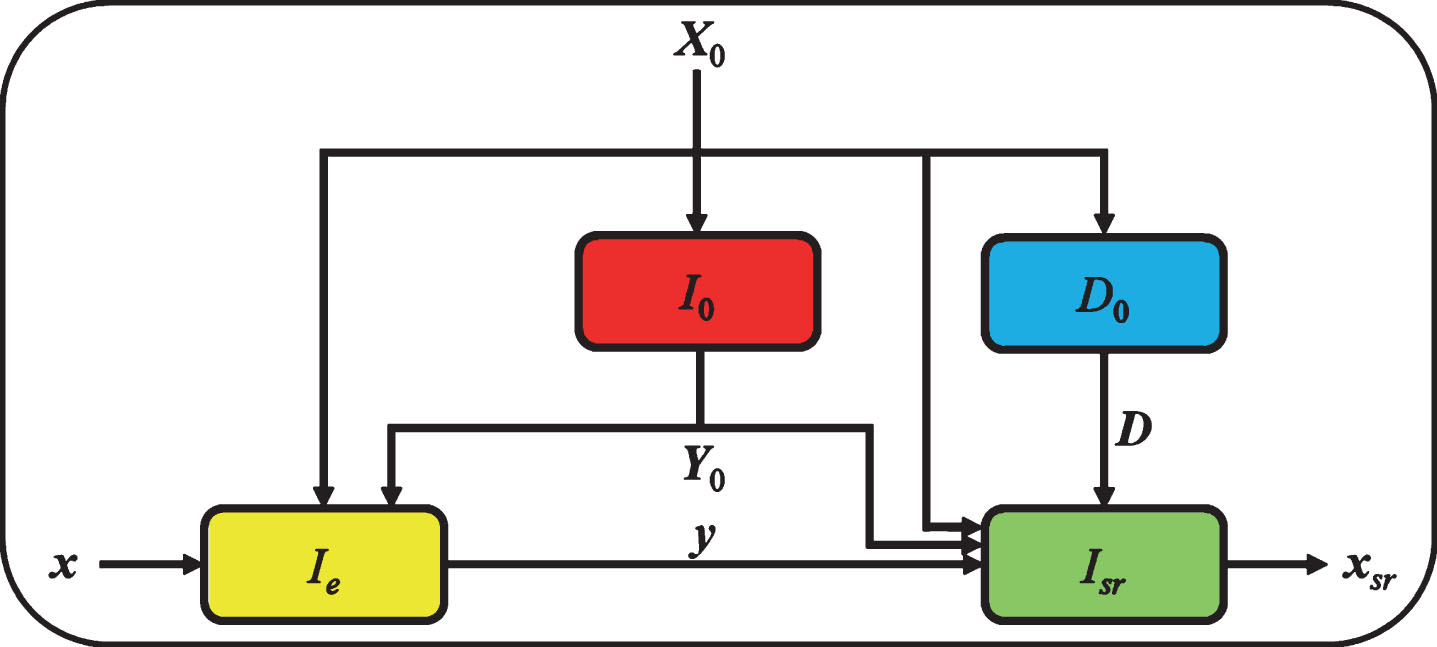
In order to promote the reconstruction performance of the general ISOMAP reconstruction architecture by making use of sparse priors of HD data, the sparse ISOMAP reconstruction architecture is shown in Fig. 2, where: D₀ is the sparse dictionary learning algorithm, which will be described later; D is the learned sparse dictionary; I_sr is the sparse ISOMAP reconstruction algorithm, which will be depicted later; X _sr is the high dimensional reconstructionsample.

Fig.2

The sparse ISOMAP reconstruction architecture.

3.2.1 Training data pair

The training data pair, which comprises the HD data and the corresponding LD data, is described by the following formulas: $\begin{matrix} P_{0} = {X_{0}, Y_{0}} = {X_{0}, Y_{0}} \\ = {x_{01}, x_{02}, \dots, x_{0 N}; y_{01}, y_{02}, \dots, y_{0 N}} \\ Y_{0} = I_{0} (X_{0}), Y_{0} = I_{0} (X_{0}), y_{0 i} = I_{0} (x_{0 i}) \\ X_{0} = [\begin{matrix} x_{01} & x_{02} & \dots & x_{0 N} \end{matrix}], X_{0} = {x_{01}, x_{02}, \dots, x_{0 N}} \\ Y_{0} = [\begin{matrix} y_{01} & y_{02} & \dots & y_{0 N} \end{matrix}], Y_{0} = {y_{01}, y_{02}, \dots, y_{0 N}} \\ X_{0} \in R^{D \times N}, x_{0 i} \in R^{D \times 1}, Y_{0} \in R^{d \times N}, y_{0 i} \in R^{d \times 1} \\ i = 1, 2, \dots, N; D > > d \end{matrix}$ (12) where: P₀ is the training pair, which contains the HD data and the related LD data, and the LD data is computed by the classical ISOMAP algorithm; I₀ is the classical ISOMAP algorithm; X ₀ is the matrix of HD training data, whose columns include HD samples; Y ₀ is the matrix of LD training data, whose columns contain LD samples; X₀ is the set version of X ₀; Y₀ is the set version of Y ₀; X _0i is the i-th column vector of X ₀; Y _0i is the i-th column vector of Y ₀; D is the dimension of HD sample; d is the dimension of LD sample; N is the total number of column vector of X ₀ or Y ₀.

3.2.2 General ISOMAP embedding algorithm

For a given HD testing sample, its LD embedding can be attained by general ISOMAP embedding algorithm, which tries to retain the distances from the LD embedding sample to its neighbors as those from the corresponding HD sample to its neighbors, and is depicted by the subsequent minimization problem: $\begin{matrix} y = I_{e} (x, X_{0}, Y_{0}) = \underset{y}{arg min} φ_{e} (x, X_{0}, Y_{0}; y) \\ = \underset{y}{arg min} \sum_{k = 1}^{K} {({∥ y - y_{k} ∥}_{2} - {∥ x - x_{k} ∥}_{2})}^{2} \\ y_{k} = I_{0} (x_{k}) \\ x_{k} \in N_{K} (x) \subset X_{0} \Rightarrow y_{k} \in N_{K} (y) \subset Y_{0} \\ N_{K} (x) = {x_{1}, x_{2}, \dots, x_{K}} \Rightarrow N_{K} (y) = {y_{1}, y_{2}, \dots, y_{K}} \\ x = {[\begin{matrix} x_{1} & x_{2} & \dots & x_{D} \end{matrix}]}^{T} \in R^{D \times 1}, \\ y = {[\begin{matrix} y_{1} & y_{2} & \dots & y_{d} \end{matrix}]}^{T} \in R^{d \times 1} \\ x_{k} = {[\begin{matrix} x_{k 1} & x_{k 2} & \dots & x_{kD} \end{matrix}]}^{T} \in R^{D \times 1}, \\ y_{k} = {[\begin{matrix} y_{k 1} & y_{k 2} & \dots & y_{kd} \end{matrix}]}^{T} \in R^{d \times 1} \\ k = 1, 2, \dots, K; K \in Z \end{matrix}$ (13) where: I_e is the general ISOMAP embedding algorithm; X is the HD testing sample; Y is the related LD embedding sample; φ_e is the object function of the minimization problem; N_k ( X ) is the set of K nearest neighbors of X in set X ₀; N_k ( Y ) is the related set of K nearest neighbors of Y in set Y ₀; X _k is the k-th vector element of N_k ( X ); Y _k is the related k-th vector element of N_k ( Y ).

3.2.3 General ISOMAP reconstruction algorithm

For a given LD testing sample, its HD reconstruction can be achieved by general ISOMAP reconstruction algorithm, which attempts to maintain the distances from the HD reconstructed sample to its neighbors as those from the related LD sample to its neighbors, and is expressed by the following minimization problem: $\begin{matrix} x_{r} = x = I_{r} (y, X_{0}, Y_{0}) = \underset{x}{arg min} φ_{r} (y, X_{0}, Y_{0}; x) \\ = \underset{x}{arg min} \sum_{k = 1}^{K} {({∥ x - x_{k} ∥}_{2} - {∥ y - y_{k} ∥}_{2})}^{2} \\ y_{k} = I_{0} (x_{k}) \\ y_{k} \in N_{K} (y) \subset Y_{0} \Rightarrow x_{k} \in N_{K} (x) \subset X_{0} \\ N_{K} (y) = {y_{1}, y_{2}, \dots, y_{K}} \Rightarrow N_{K} (x) = {x_{1}, x_{2}, \dots, x_{K}} \\ y = {[\begin{matrix} y_{1} & y_{2} & \dots & y_{d} \end{matrix}]}^{T} \in R^{d \times 1}, \\ x = {[\begin{matrix} x_{1} & x_{2} & \dots & x_{D} \end{matrix}]}^{T} \in R^{D \times 1} \\ y_{k} = {[\begin{matrix} y_{k 1} & y_{k 2} & \dots & y_{kd} \end{matrix}]}^{T} \in R^{d \times 1}, \\ x_{k} = {[\begin{matrix} x_{k 1} & x_{k 2} & \dots & x_{kD} \end{matrix}]}^{T} \in R^{D \times 1} \\ k = 1, 2, \dots, K; K \in Z \end{matrix}$ (14) where: I_r is the general ISOMAP reconstruction algorithm; Y is the LD testing sample; X is the related HD reconstruction sample; X _r is also the related HD reconstruction sample; φ_r is the object function of the minimization problem; N_k ( Y ) is the set of K nearest neighbors of Y in set Y ₀; N_k ( X ) is the related set of K nearest neighbors of X in set X ₀; Y _i is the i-th vector element of N_k ( Y ); X _i is the related i-th vector element of N_k ( X ).

3.2.4 Sparse dictionary learning algorithm

Because the general ISOMAP algorithm cannot provide a satisfied reconstruction of original HD data, the sparse priors of HD data are considered to improve the reconstruction quality. According to the training data pair, a sparse dictionary is learned by the following minimization problem: $\begin{matrix} D = D_{0} (X_{0}) = \underset{D}{arg min} \sum_{i = 1}^{N} {∥ s_{0 i} ∥}_{0}, s . t . X_{0} = {DS}_{0} \\ x_{0 i} = {Ds}_{0 i}, D = [\begin{matrix} d_{11} & d_{12} & \dots & d_{1 M} \\ d_{21} & d_{22} & \dots & d_{2_{M}} \\ ⋮ & ⋮ & ⋮ & ⋮ \\ d_{D 1} & d_{D 2} & \dots & d_{DM} \end{matrix}] \in R^{D \times M} \end{matrix}$ $\begin{matrix} S_{0} = [\begin{matrix} s_{01} & s_{02} & \dots & s_{0 N} \end{matrix}] \in R^{M \times N}, \\ s_{0 i} = {[\begin{matrix} s_{0 i 1} & s_{0 is} & \dots & s_{0 iM} \end{matrix}]}^{T} \in R^{M \times 1} \\ i = 1, 2, \dots, N \end{matrix}$ (15) where: D is the learned dictionary; D₀ is the learning algorithm of sparse dictionary, and any kinds of learning algorithm can be adopted [32]; S ₀ is the sparse coefficient matrix of X ₀; S _0i is the i-th vector column of S ₀ and is the sparse coefficient vectorof X ₀i.

3.2.5 Sparse ISOMAP reconstruction algorithm

Relying on the aforementioned sparse dictionary of HD data, the sparse ISOMAP reconstruction algorithm can be described by the following minimization problem: $\begin{matrix} x_{sr} = x = I_{sr} (y, X_{0}, Y_{0}, D) \\ (x, s) = \underset{x, s}{arg min} ψ (y, X_{0}, Y_{0}; x, s), s . t . {∥ x - Ds ∥}_{2}^{2} ⩽ ɛ \\ ψ (y, X_{0}, Y_{0}; x, s) = φ_{sr} (y, X_{0}, Y_{0}; x) + λ φ_{s} (s) \\ φ_{sr} (y, X_{0}, Y_{0}; x) = \sum_{k = 1}^{K} {({∥ y - y_{k} ∥}_{2} - {∥ x - x_{k} ∥}_{2})}^{2} \\ φ_{s} (s) = {∥ s ∥}_{0}, s = {[\begin{matrix} s_{1} & s_{s} & \dots & s_{M} \end{matrix}]}^{T} \in R^{M \times 1} \\ y_{k} = I_{0} (x_{k}) \\ x_{k} \in N_{K} (x) \subset X_{0} \Rightarrow y_{k} \in N_{K} (y) \subset Y_{0} \end{matrix}$ (16) where: ψ is the object function of the total minimization problem; φ_sr is the object function of the minimization problem for sparse ISOMAP reconstruction; φ_s is the object function of the minimization problem for sparse priors; λ is a known positive constant; S is the sparse coefficient vector of X .

The abovementioned constrained minimization problem can be rewritten as the subsequent two alternative constrained minimization problems: $\begin{matrix} x = \underset{x}{arg min} φ_{sr} (y, X_{0}, Y_{0}; x), s . t . {∥ x - Ds ∥}_{2}^{2} ⩽ ɛ \\ s = \underset{s}{arg min} φ_{s} (s), s . t . {∥ x - Ds ∥}_{2}^{2} ⩽ ɛ \end{matrix}$ (17)

They can be further rewritten as the following two alternative unconstraint minimization problems: $\begin{matrix} x = \underset{x}{arg min} φ_{sr} (y, s, X_{0}, Y_{0}, D; x) = \underset{x}{arg min} \\ \sum_{k = 1}^{K} {({∥ y - y_{k} ∥}_{2} - {∥ x - x_{k} ∥}_{2})}^{2} + α {∥ x - Ds ∥}_{2}^{2} \\ s = \underset{s}{arg min} φ_{s} (x, D; s) = \underset{s}{arg min} {∥ s ∥}_{0} + β {∥ x - Ds ∥}_{2}^{2} \end{matrix}$ (18) where: φ_sr is the object function of the minimization problem for sparse ISOMAP reconstruction; φ_s is the object function of the minimization problem for sparse priors; α is a known positive constant; β is a known positive constant.

The derivative of φ_sr with respect to X can be expressed by the subsequent equations: $\begin{matrix} \frac{\partial}{\partial x} φ_{sr} = {[\begin{matrix} \frac{\partial}{\partial x_{1}} φ_{sr} & \frac{\partial}{\partial x_{2}} φ_{sr} & \dots & \frac{\partial}{\partial x_{D}} φ_{sr} \end{matrix}]}^{T} \\ \frac{\partial}{\partial x_{i}} φ_{sr} = \frac{\partial}{\partial x_{i}} (\sum_{k = 1}^{K} {({∥ y - y_{k} ∥}_{2} - {∥ x - x_{k} ∥}_{2})}^{2} + α {∥ x - Ds ∥}_{2}^{2}) \\ = \frac{\partial}{\partial x_{i}} (\sum_{k = 1}^{K} {(\sqrt{\sum_{j = 1}^{d} {(y_{j} - y_{kj})}^{2}} - \sqrt{\sum_{j = 1}^{D} {(x_{j} - x_{kj})}^{2}})}^{2} \\ + α \sum_{j = 1}^{D} {(x_{j} - \sum_{l = 1}^{M} d_{jl} s_{l})}^{2}) \\ = - 2 \sum_{k = 1}^{K} \frac{(x_{i} - x_{ki}) (\sqrt{\sum_{j = 1}^{d} {(y_{j} - y_{kj})}^{2}} - \sqrt{\sum_{j = 1}^{D} {(x_{j} - x_{kj})}^{2}})}{\sqrt{\sum_{j = 1}^{D} {(x_{j} - x_{kj})}^{2}}} \\ + 2 α (x_{i} - \sum_{l = 1}^{M} d_{il} s_{l}) \\ = - 2 \sum_{k = 1}^{K} \frac{(x_{i} - x_{ki}) ({∥ y - y_{k} ∥}_{2} - {∥ x - x_{k} ∥}_{2})}{{∥ x - x_{k} ∥}_{2}} \\ + 2 α (x_{i} - \sum_{l = 1}^{M} d_{il} s_{l}), i = 1, 2, \dots, D \end{matrix}$ (19)

The derivative of φ_s with respect to s can be described by the following formulas: $\begin{matrix} \frac{\partial}{\partial s} φ_{s} = {[\begin{matrix} \frac{\partial}{\partial s_{1}} φ_{s} & \frac{\partial}{\partial s_{2}} φ_{s} & \dots & \frac{\partial}{\partial s_{M}} φ_{s} \end{matrix}]}^{T} \\ \frac{\partial}{\partial s_{i}} φ_{s} = \frac{\partial}{\partial s_{i}} ({∥ s ∥}_{0} + β {∥ x - Ds ∥}_{2}^{2}) \\ \approx \frac{\partial}{\partial s_{i}} ({∥ s ∥}_{1} + β {∥ x - Ds ∥}_{2}^{2}) \\ = \frac{\partial}{\partial s_{i}} (\sum_{j = 1}^{M} | s_{j} | + β \sum_{j = 1}^{D} {(x_{j} - \sum_{l = 1}^{M} d_{jl} s_{l})}^{2}) \end{matrix}$ $\begin{matrix} = \frac{\partial}{\partial s_{i}} (\sum_{j = 1}^{M} s_{j} sign (s_{j}) + β \sum_{j = 1}^{D} {(x_{j} - \sum_{l = 1}^{M} d_{jl} s_{l})}^{2}) \\ \approx \frac{\partial}{\partial s_{i}} (\sum_{j = 1}^{M} s_{j} tanh (s_{j}) + β \sum_{j = 1}^{D} {(x_{j} - \sum_{l = 1}^{M} d_{jl} s_{l})}^{2}) \\ = \frac{\partial}{\partial s_{i}} (\sum_{j = 1}^{M} s_{j} \frac{e^{s_{j}} - e^{- s_{j}}}{e^{s_{j}} + e^{- s_{j}}} + β \sum_{j = 1}^{D} {(x_{j} - \sum_{l = 1}^{M} d_{jl} s_{l})}^{2}) \\ = \frac{e^{s_{i}} - e^{- s_{i}}}{e^{s_{i}} + e^{- s_{i}}} + \frac{4 s_{i}}{{(e^{s_{i}} + e^{- s_{i}})}^{2}} - 2 β \sum_{j = 1}^{D} d_{ji} (x_{j} - \sum_{l = 1}^{M} d_{jl} s_{l}) \\ = tanh (s_{i}) + \frac{s_{i}}{{cosh}^{2} (s_{i})} - 2 β \sum_{j = 1}^{D} d_{ji} (x_{j} - \sum_{l = 1}^{M} d_{jl} s_{l}), \\ i = 1, 2, \dots, M \end{matrix}$ (20)

Hence, the foregoing alternative unconstrained minimization problems can be resolved by the following alternative standard gradient descent procedures: $x = x - μ \frac{\partial}{\partial x} φ_{sr}, s = s - η \frac{\partial}{\partial s} φ_{s}$ (21) where: μ is a known positive constant; η is also a known positive constant.

Finally, the sparse reconstruction sample of ISOMAP representation is gained by the following formula: $x_{sr} = x$ (22)

3.3 Description of sparse ISOMAP reconstruction algorithm

The description of the sparse ISOMAP reconstruction algorithm is listed in Table 1.

Table 1
The description of the sparse ISOMAP reconstruction algorithm

Sparse ISOMAP reconstruction algorithm

Input: X ₀, X

     Initialize: Y ₀ = I₀ ( X ₀), D = D₀ ( X ₀), Y = I_e ( X )

     while not converged do

         compute X according to formula (19) and (21)

         compute S according to formula (20) and (21)

     end while

Output: X _sr = X

Sparse ISOMAP reconstruction algorithm
Input: X ₀, X
Initialize: Y ₀ = I₀ ( X ₀), D = D₀ ( X ₀), Y = I_e ( X )
while not converged do
compute X according to formula (19) and (21)
compute S according to formula (20) and (21)
end while
Output: X _sr = X

4 Experiments

4.1 Experimental conditions

Three experiments are designed to evaluate the performance of the proposed method. The first is the experiment of image reconstruction, the second is the experiment of video reconstruction, and the third is the experiment of signal reconstruction.

The experimental images come from the University of Southern California - Signal and Image Processing Institute (USC-SIPI) image database (http://sipi.usc.edu/database/database.php). It has four volumes: Textures, Aerials, Miscellaneous, and Sequences. The first three volumes are employed for the experiment of image reconstruction, and the last volume is applied to the experiment of video reconstruction. All color images are converted into grayscale images, and the image size is adjusted to 256×256. Each image is partitioned into small blocks with same size 8×8.

The experimental videos are also derived from the testing sequences of highly efficient video coding (HEVC) [31]. The HEVC testing sequences comprises five subsets: A, B, C, D, and E, and only subset D is adopted for the experiment. All color frames are transformed into grayscale frames, and the frame size is 240×416. Each frame is divided into small patches with the same size 8×8.

The experimental signals are chosen from the Apnea-Electrocardiograph (Apnea-ECG) Database (https://www.physionet.org/physiobank/database/apnea-ecg/) [32, 33]. Only 20 records, a01-a20, are selected for experiment from the total 70 records. Each record is divided into fragments with same size, and each fragment holds 90 sampling data points, which is corresponding to a cycle of ECG signal. Each fragment is normalized by peak alignment. For each record, the first 1024 chips are utilized as training samples, and the second 1024 chips are utilized as testing samples.

The proposed method is compared with two state-of-the-art methods of image and video coding: sparse representation (SR) [34] and discrete cosine transformation (DCT) [35]. The SR algorithm is K-SVD, the size of sparse dictionary is 256, the sparse level is arbitrary, the number of iterations is 20, the stop criterion is a given representation error, and the algorithm of sparse coefficients estimation is orthogonal matching pursuit (OMP) [34]. The DCT algorithm is direct discrete cosine transform and dictionary learning of DCT is not exploited [35].

This paper is devoted to the situation of LD representations of HD data, such as 1D, 2D and 3D LD representations. For the proposed method, one, two or three LD ISOMAP representations of image patches are employed for reconstruction. For SR, the most important one, two or three sparse coefficients of image patches are preserved for reconstruction. For DCT, the most important one, two or three DCT coefficients of image patches are retained for reconstruction.

The experimental hardware platform is a laptop computer with 2.6 GHz CPU and 8GB memory, and the experimental software platform is Matlab 2016a on Windows 10.

4.2 Experiment of image reconstruction

The experiment of image reconstruction is devised as self embedding and reconstruction. That is to say: an image is utilized to establish a training set and then the same image is rebuilt from the training set. The reason for this design is that, we expect to preliminarily verify the reconstruction performance of the proposed method. The usage of different training and testing samples is probed in the following experiment of video reconstruction.

The experimental results of the USC-SIPI image database are listed in Tables 2–4, which respectively enumerate the results of the aerials volume, miscellaneous volume and textures volume. It is revealed in Tables 2–4 that, the proposed method is superior to DCT and SR in the peak signal to noise ratio (PSNR) of image reconstruction, in the situation of the 2D and 3D LD representations. It is also indicated in Tables 2–4 that, the average PSNRs of miscellaneous volume are higher than those of aerials volume, in the case of 2D and 3D LD representations. This is because that the images in aerials volume hold more details than those of miscellaneous volume. It is further reflected in Tables 2–4 that, the average PSNR of textures volume is higher than that of miscellaneous volume, in the situation of 3D LD representation. This is due to that fact that, the images of textures volume possess more repeated patches than those of miscellaneous volume and the ISOMAP algorithm depends on the similarities between image patches, although the former holds more details than the latter.

Table 2
The experimental results of the aerials volume of USC-SIPI image database

Image PSNR (dB)

1D 2D 3D

DCT SR Proposed DCT SR Proposed DCT SR Proposed

2.1.01 18.9757 18.5806 16.2323 19.4770 19.0741 27.4991 20.3375 20.0438 40.1441

2.1.02 16.8702 16.4950 13.9907 17.3226 17.0199 22.7338 17.8136 17.3416 37.7566

2.1.03 25.5803 25.1138 22.7310 26.0741 25.6546 31.5661 26.6109 26.2448 39.5912

2.1.04 21.8206 21.5012 18.8122 22.1670 21.7205 24.9293 22.5491 22.1230 37.4992

2.1.05 17.4885 17.0689 14.7546 18.1341 17.7707 25.6164 19.0744 18.6495 37.3402

2.1.06 18.5105 18.1439 15.4990 18.9784 18.4837 25.1244 19.5436 19.1680 39.8139

2.1.07 24.2987 24.0982 21.4193 24.8036 24.4286 27.9390 25.4558 25.2294 36.3966

2.1.08 22.9627 22.4866 20.0293 23.3578 23.0006 24.7875 23.9347 23.5468 38.8253

2.1.09 25.2261 25.1244 22.3007 26.0884 26.0075 30.4460 26.7589 26.6994 38.6101

2.1.10 21.1069 21.0849 17.9230 21.4837 21.3895 24.4288 21.8597 21.7640 37.9764

2.1.11 20.1420 20.0615 17.3488 21.0656 20.6026 28.3686 21.9598 21.6820 40.1456

2.1.12 22.2958 22.0087 19.2411 22.7330 22.3225 23.9284 23.2411 23.0125 37.4777

2.2.01 19.5025 19.1366 16.6134 20.0857 19.6381 25.8358 20.6320 20.5879 35.5807

2.2.02 26.4103 26.0789 23.3896 27.2622 27.0270 30.3479 28.3800 28.0533 39.9418

2.2.03 25.0485 24.6846 22.1073 25.5555 25.0989 25.7404 26.2904 26.0334 35.6176

2.2.04 21.7842 21.3798 18.8333 22.1659 22.0108 23.1460 22.5971 22.2150 32.5312

2.2.05 18.6389 18.2630 15.7780 19.1174 19.0993 26.2203 19.9480 19.5842 40.9937

2.2.06 27.3263 27.0529 24.4157 27.7042 27.3718 30.4391 28.1740 28.0227 38.6282

2.2.07 24.9063 24.4267 21.8383 25.3353 25.0073 25.6056 26.1956 26.0777 36.0753

2.2.08 19.4987 19.0275 16.4402 20.0525 19.6375 25.5915 20.6314 20.2104 36.6534

2.2.09 24.3992 24.0724 21.6412 25.0153 24.7447 27.1196 25.5109 25.2272 37.5987

2.2.10 25.8951 25.6386 22.8167 26.4838 26.1982 28.4162 27.0721 26.8819 38.0510

2.2.11 22.3942 22.0757 19.4312 22.8473 22.5636 25.0850 23.4187 23.1717 42.0098

2.2.12 25.0840 24.8517 22.0478 25.5947 25.1361 27.8704 26.3432 26.0853 39.3786

2.2.13 25.7026 25.5110 22.5681 26.2008 26.0132 27.4014 26.7513 26.4248 35.5582

2.2.14 22.9548 22.8507 20.0140 23.4176 23.2250 24.6379 24.0003 23.8571 35.9503

2.2.15 25.1457 25.0245 22.2019 25.6921 25.4252 28.4763 26.2650 26.1118 40.0963

2.2.16 22.5119 22.2456 19.4241 22.9797 22.6494 25.3863 23.5055 23.1975 34.2248

2.2.17 18.9009 18.7673 15.9088 19.1270 19.0055 23.8533 19.3667 19.2548 36.7086

2.2.18 21.9916 21.6746 19.0019 22.4817 22.1271 25.7866 23.1785 23.0015 40.2221

2.2.19 24.3610 24.2328 21.4917 24.9038 24.6534 26.0832 25.5776 25.3047 39.4813

2.2.20 22.4628 22.2235 19.6124 23.0977 22.7577 28.0103 23.7047 23.5776 40.1588

2.2.21 22.4622 22.1712 19.3875 23.1095 22.9417 25.4602 23.6594 23.3423 33.8811

2.2.22 25.2658 25.0026 22.3787 25.8285 25.6488 27.8193 26.5161 26.3414 38.3942

2.2.23 27.4491 27.2062 24.5577 28.0054 27.9696 30.7171 28.9719 28.4379 39.7435

2.2.24 26.0628 25.8187 23.2252 26.6491 26.1064 27.7377 27.4941 27.1886 34.9448

3.2.25 21.0703 20.6951 18.1160 21.7513 21.3708 25.6548 22.4102 22.2947 40.3575

wash-ir 18.0226 17.8294 15.1004 18.4324 18.2746 22.4290 18.9225 18.7952 34.8720

Average 22.6455 22.4832 19.7006 23.1732 22.8731 26.5326 23.8067 23.5470 37.8745

Image	PSNR (dB)
2.1.01	18.9757	18.5806	16.2323	19.4770	19.0741	27.4991	20.3375	20.0438	40.1441
2.1.02	16.8702	16.4950	13.9907	17.3226	17.0199	22.7338	17.8136	17.3416	37.7566
2.1.03	25.5803	25.1138	22.7310	26.0741	25.6546	31.5661	26.6109	26.2448	39.5912
2.1.04	21.8206	21.5012	18.8122	22.1670	21.7205	24.9293	22.5491	22.1230	37.4992
2.1.05	17.4885	17.0689	14.7546	18.1341	17.7707	25.6164	19.0744	18.6495	37.3402
2.1.06	18.5105	18.1439	15.4990	18.9784	18.4837	25.1244	19.5436	19.1680	39.8139
2.1.07	24.2987	24.0982	21.4193	24.8036	24.4286	27.9390	25.4558	25.2294	36.3966
2.1.08	22.9627	22.4866	20.0293	23.3578	23.0006	24.7875	23.9347	23.5468	38.8253
2.1.09	25.2261	25.1244	22.3007	26.0884	26.0075	30.4460	26.7589	26.6994	38.6101
2.1.10	21.1069	21.0849	17.9230	21.4837	21.3895	24.4288	21.8597	21.7640	37.9764
2.1.11	20.1420	20.0615	17.3488	21.0656	20.6026	28.3686	21.9598	21.6820	40.1456
2.1.12	22.2958	22.0087	19.2411	22.7330	22.3225	23.9284	23.2411	23.0125	37.4777
2.2.01	19.5025	19.1366	16.6134	20.0857	19.6381	25.8358	20.6320	20.5879	35.5807
2.2.02	26.4103	26.0789	23.3896	27.2622	27.0270	30.3479	28.3800	28.0533	39.9418
2.2.03	25.0485	24.6846	22.1073	25.5555	25.0989	25.7404	26.2904	26.0334	35.6176
2.2.04	21.7842	21.3798	18.8333	22.1659	22.0108	23.1460	22.5971	22.2150	32.5312
2.2.05	18.6389	18.2630	15.7780	19.1174	19.0993	26.2203	19.9480	19.5842	40.9937
2.2.06	27.3263	27.0529	24.4157	27.7042	27.3718	30.4391	28.1740	28.0227	38.6282
2.2.07	24.9063	24.4267	21.8383	25.3353	25.0073	25.6056	26.1956	26.0777	36.0753
2.2.08	19.4987	19.0275	16.4402	20.0525	19.6375	25.5915	20.6314	20.2104	36.6534
2.2.09	24.3992	24.0724	21.6412	25.0153	24.7447	27.1196	25.5109	25.2272	37.5987
2.2.10	25.8951	25.6386	22.8167	26.4838	26.1982	28.4162	27.0721	26.8819	38.0510
2.2.11	22.3942	22.0757	19.4312	22.8473	22.5636	25.0850	23.4187	23.1717	42.0098
2.2.12	25.0840	24.8517	22.0478	25.5947	25.1361	27.8704	26.3432	26.0853	39.3786
2.2.13	25.7026	25.5110	22.5681	26.2008	26.0132	27.4014	26.7513	26.4248	35.5582
2.2.14	22.9548	22.8507	20.0140	23.4176	23.2250	24.6379	24.0003	23.8571	35.9503
2.2.15	25.1457	25.0245	22.2019	25.6921	25.4252	28.4763	26.2650	26.1118	40.0963
2.2.16	22.5119	22.2456	19.4241	22.9797	22.6494	25.3863	23.5055	23.1975	34.2248
2.2.17	18.9009	18.7673	15.9088	19.1270	19.0055	23.8533	19.3667	19.2548	36.7086
2.2.18	21.9916	21.6746	19.0019	22.4817	22.1271	25.7866	23.1785	23.0015	40.2221
2.2.19	24.3610	24.2328	21.4917	24.9038	24.6534	26.0832	25.5776	25.3047	39.4813
2.2.20	22.4628	22.2235	19.6124	23.0977	22.7577	28.0103	23.7047	23.5776	40.1588
2.2.21	22.4622	22.1712	19.3875	23.1095	22.9417	25.4602	23.6594	23.3423	33.8811
2.2.22	25.2658	25.0026	22.3787	25.8285	25.6488	27.8193	26.5161	26.3414	38.3942
2.2.23	27.4491	27.2062	24.5577	28.0054	27.9696	30.7171	28.9719	28.4379	39.7435
2.2.24	26.0628	25.8187	23.2252	26.6491	26.1064	27.7377	27.4941	27.1886	34.9448
3.2.25	21.0703	20.6951	18.1160	21.7513	21.3708	25.6548	22.4102	22.2947	40.3575
wash-ir	18.0226	17.8294	15.1004	18.4324	18.2746	22.4290	18.9225	18.7952	34.8720
Average	22.6455	22.4832	19.7006	23.1732	22.8731	26.5326	23.8067	23.5470	37.8745

Table 3

The experimental results of the miscellaneous volume of USC-SIPI image database

Image	PSNR (dB)
	1D			2D			3D
	DCT	SR	Proposed	DCT	SR	Proposed	DCT	SR	Proposed
4.1.01	25.6562	25.4073	22.8978	26.7095	26.4546	33.7414	28.8986	28.5757	42.0232
4.1.02	27.0566	26.7305	24.3115	28.9348	28.8942	33.2652	30.0006	29.7214	40.4818
4.1.03	23.0239	22.9203	23.7298	23.4411	23.1784	35.3471	27.6859	27.4340	41.9144
4.1.04	20.2048	19.6534	19.9168	24.1561	24.0655	31.3357	26.5044	26.3615	42.3534
4.1.05	21.6820	21.3035	19.2463	22.5370	22.2613	34.3267	24.6788	24.2922	40.4667
4.1.06	17.9522	17.2138	15.1374	18.8775	18.7173	31.2641	21.2872	21.1942	41.6393
4.1.07	24.2383	24.0655	21.6394	26.3340	26.1392	39.1530	28.5183	28.3755	43.7552
4.1.08	21.7651	21.5081	18.6758	23.7008	23.3892	34.6380	26.3266	26.0787	44.2586
4.2.01	22.0577	21.7647	20.2771	23.2769	23.0461	31.9061	24.7846	24.3646	37.8882
4.2.03	19.2699	14.4595	16.3819	19.7769	14.1418	23.8714	20.2106	14.4016	37.1308
4.2.05	18.1858	18.0041	15.4419	19.0470	18.8439	28.8016	20.3667	20.1152	42.0618
4.2.06	17.6291	17.1887	14.9291	18.3662	18.0438	27.4748	19.8856	19.6012	37.7102
4.2.07	19.9550	19.4896	17.0459	21.5262	21.109	30.3680	23.2846	23.0807	42.8368
5.1.09	25.9338	25.6572	23.5002	27.3883	27.1773	30.1867	28.1635	28.0212	40.4564
5.1.10	17.9406	17.7469	15.1503	18.6385	18.1086	28.0566	20.4673	20.0657	46.0898
5.1.11	24.4167	24.3506	22.9151	25.1741	25.0994	33.0979	26.4305	26.1274	41.8596
5.1.12	20.9894	20.4191	18.5773	22.4244	22.0398	30.7945	23.9185	23.8684	40.1568
5.1.13	13.1353	13.0809	11.8773	14.2895	14.1929	32.2871	15.8684	15.4830	43.3187
5.1.14	20.7598	20.3000	18.0119	21.5331	21.4065	29.8988	22.8815	22.6731	40.7110
5.2.08	19.8624	19.6591	18.1511	20.3826	20.1884	27.6245	22.0273	21.8481	38.8298
5.2.09	17.2465	17.9211	14.3627	17.7127	17.4119	24.2763	18.4614	18.8474	37.1807
5.2.10	18.3478	18.2980	15.6948	18.9352	18.7484	26.7986	20.3259	20.0149	40.1710
5.3.01	18.3896	18.2783	15.3973	19.4709	19.3494	26.5882	20.5554	20.4988	39.4870
5.3.02	19.8676	19.7898	17.0061	20.6190	20.1099	26.2053	21.1358	21.0963	36.9937
7.1.01	23.6722	23.5780	20.8889	24.1720	23.8910	28.7672	25.6148	25.3668	35.1666
7.1.02	25.0238	24.8406	23.9150	26.0940	25.7465	34.6201	26.7548	26.4136	38.6708
7.1.03	25.2113	24.9676	22.1568	25.9848	25.8142	29.0988	27.0568	26.8004	40.0297
7.1.04	24.5239	24.4925	21.7915	25.1121	25.0159	28.5551	26.4905	26.0638	37.5469
7.1.05	21.4604	21.1270	18.5557	21.9327	21.8900	29.5453	23.4977	22.8556	42.8275
7.1.06	21.4252	21.2559	18.5229	21.8401	21.7726	31.1872	23.5783	23.0031	44.0847
7.1.07	23.2999	23.0388	20.4841	23.7439	23.5097	29.4306	24.8176	24.5942	43.4871
7.1.08	26.8296	26.3910	24.3660	27.4885	27.1456	30.2598	28.6600	28.4649	36.9709
7.1.09	23.5481	23.4427	20.5988	24.0052	23.7467	28.9994	25.1999	25.0745	40.4600
7.1.10	24.2235	24.0294	21.3445	24.6597	24.3322	30.2169	26.4767	26.2999	40.3549
7.2.01	26.8092	26.6445	25.0910	28.3300	28.0349	35.5166	29.3723	29.2398	37.5799
boat	19.6535	19.2602	16.9652	20.3349	20.1343	26.1544	21.7758	21.3291	44.8137
gray21	26.1787	26.0682	11.6973	31.6382	31.5335	32.0590	32.0005	31.9676	47.9501
house	18.5534	18.0588	15.8258	19.2977	19.1657	26.3838	20.3814	20.1925	40.8301
ruler	14.1849	14.0706	17.9177	14.3832	14.2641	18.3471	14.6263	14.5162	29.3592
Average	21.5427	21.1834	18.9845	22.6223	22.2296	30.0115	24.0762	23.7006	40.5104

Table 4

The experimental results of the textures volume of USC-SIPI image database

Image	PSNR (dB)
	1D			2D			3D
	DCT	SR	Proposed	DCT	SR	Proposed	DCT	SR	Proposed
1.1.01	13.6191	13.4716	10.7768	13.8848	13.6403	23.6544	14.1834	14.0182	46.0396
1.1.02	15.1092	15.0498	12.1155	15.9156	15.7314	26.9922	16.3399	16.2801	46.8078
1.1.03	16.3321	16.1522	13.5758	16.5539	16.4934	22.1140	16.8252	16.6184	44.9668
1.1.04	17.6652	17.2895	15.1672	17.7314	17.5713	29.2199	17.8893	17.7461	43.6605
1.1.05	20.9675	20.5597	18.1678	21.3823	21.1983	27.5214	21.8993	21.6299	44.5532
1.1.06	16.0972	15.9758	13.3873	16.4279	16.2473	27.0202	16.5664	16.4657	46.2553
1.1.07	18.8609	18.6864	15.8675	19.0873	18.9278	23.9671	19.4495	19.1961	47.7251
1.1.08	24.6727	24.5365	23.7321	24.8849	24.7131	27.6800	25.5205	25.2621	43.9185
1.1.09	20.2801	20.0664	17.2858	20.7295	20.6735	26.7300	21.0031	20.9692	46.7180
1.1.10	18.3276	18.2037	15.7712	18.5723	18.4632	26.3675	18.9299	18.8479	45.2566
1.1.11	19.8541	19.3598	18.4411	20.0702	19.7480	25.6604	21.7531	21.5720	41.9525
1.1.12	18.7586	18.6934	16.7877	19.9574	19.8199	29.1125	20.1922	20.0781	42.0592
1.1.13	17.0249	16.8363	14.2191	17.6682	17.4799	27.6916	18.3601	18.2536	46.3391
1.2.01	11.1123	11.0925	08.2439	11.3800	11.2174	25.3364	11.6674	11.5251	45.6394
1.2.02	11.4533	11.0845	08.6513	12.2579	12.1555	30.5463	12.6719	12.5168	45.6304
1.2.03	11.1140	11.0968	08.2228	11.3320	11.2256	26.7291	11.5625	11.4609	45.6037
1.2.04	10.1893	10.0545	07.9228	10.2536	10.1426	28.3583	10.3209	10.2844	45.4971
1.2.05	12.2712	12.1982	09.4841	12.7276	12.4998	26.3896	13.1558	13.0197	45.6556
1.2.06	10.8917	10.5038	08.2735	11.2575	11.0103	26.5608	11.3757	11.2153	45.7323
1.2.07	10.8956	10.5024	08.0190	11.1451	11.0502	23.6792	11.4235	11.2224	45.6811
1.2.08	11.6876	11.4711	08.7465	12.0103	11.8213	28.1524	12.1995	12.0588	45.7254
1.2.09	12.0430	11.8422	09.0235	12.6783	12.5513	26.7559	12.7750	12.6435	45.8064
1.2.10	10.7382	10.0323	07.8587	11.0064	10.9042	30.6530	11.2908	11.0313	45.5937
1.2.11	11.1786	10.7283	08.5047	11.5128	11.3686	25.7931	12.0705	11.9740	45.6637
1.2.12	12.8232	12.6707	10.1860	13.8898	13.3065	28.6915	14.0567	13.9343	45.9385
1.2.13	11.7733	11.1455	08.9701	12.4541	12.3659	29.4652	13.1686	13.0756	45.5804
1.3.01	14.5937	14.2734	11.6612	14.8765	14.6333	23.3138	15.1547	15.0667	46.5399
1.3.02	15.7209	15.6481	12.8489	16.7094	16.6889	28.0979	17.1303	17.0518	44.7957
1.3.03	16.2496	15.8791	13.2787	16.8520	16.2961	25.4774	16.9723	16.5471	43.9683
1.3.04	17.3876	17.1849	14.5410	18.0238	17.8056	27.4885	18.5603	18.4791	46.0312
1.3.05	12.8826	12.6626	10.4636	13.0219	12.8038	27.9041	13.1555	13.0927	45.7647
1.3.06	16.2767	16.1565	13.3448	16.7062	16.5969	25.719	16.8489	16.8115	46.5556
1.3.07	18.8533	18.1108	15.8411	19.2028	19.0339	24.6163	19.6095	19.5631	40.1511
1.3.08	26.9945	26.2361	24.7582	27.3977	27.0622	28.7983	27.5345	27.3503	42.9331
1.3.09	20.8132	20.6739	18.7938	21.5843	21.1699	29.0079	21.6356	21.3614	47.4641
1.3.10	21.0359	20.8627	18.1384	21.6038	21.3836	27.3752	21.9805	21.8519	47.1144
1.3.11	20.9963	20.2774	18.0325	21.4231	21.3684	26.7974	21.9525	21.6334	47.9848
1.3.12	20.0174	19.6464	18.2698	21.0186	20.7106	27.1120	21.1237	21.0457	39.2804
1.3.13	18.0335	17.7760	15.1035	18.6920	18.1321	27.3232	19.4599	19.1643	47.1242
1.4.01	19.9203	18.8592	16.0565	19.9727	19.2198	29.3567	20.8758	20.6870	44.1008
1.4.02	15.1723	15.0162	12.6407	15.2426	15.1092	30.9138	16.2339	16.1245	40.9420
1.4.03	18.1030	17.8141	14.9613	18.1760	18.0504	31.3132	19.9269	19.6922	40.7020
1.4.04	26.3061	25.9226	23.6960	26.6182	26.4926	31.8415	27.8752	27.3778	42.9386
1.4.05	19.5093	19.1677	14.3504	19.7908	19.512	32.4056	21.4521	21.2362	37.7202
1.4.06	22.1661	21.8153	20.1656	22.7778	22.0919	26.6381	23.9922	23.4121	43.8256
1.4.07	22.7667	21.8740	20.2936	22.8290	22.5837	27.7306	23.5277	23.4587	40.1742
1.4.08	21.5421	21.0026	16.4918	21.6283	21.5593	27.2927	22.8218	22.2662	42.5771
1.4.09	16.2508	15.9063	14.2270	17.1423	16.8243	31.6312	17.5401	17.0502	42.3236
1.4.10	20.2500	20.0323	17.4795	20.4204	20.2866	21.3773	20.8891	20.3093	37.7269
1.4.11	19.6842	18.8781	16.9819	19.7769	19.3609	23.0530	20.2796	20.1918	31.7816
1.4.12	20.5397	20.2382	17.8355	20.6273	20.4425	24.6883	20.8600	20.6478	38.3090
1.5.01	24.3204	24.3517	22.1451	24.9964	24.5561	29.3320	25.5179	25.3867	38.1827
1.5.02	07.9213	11.2976	06.9893	08.0129	12.1616	30.0284	08.0930	13.0130	44.5095
1.5.03	18.3642	17.5232	15.4991	19.4297	18.9922	27.5913	20.1115	19.6812	46.4285
1.5.04	19.7279	19.4943	16.7305	19.9298	19.8744	22.5025	20.1645	20.0854	44.0362
1.5.05	18.5949	18.1718	15.6892	19.6406	19.0619	28.2193	20.8716	20.4893	44.7595
1.5.06	30.7558	29.0584	28.5448	30.8175	30.2825	32.5744	31.5325	31.0457	39.1182
1.5.07	19.8295	19.7599	16.8857	20.1929	20.0428	24.4196	20.4769	20.3546	42.7132
texmos1.p	11.1923	10.6056	08.2166	11.5359	11.0886	26.8556	11.8255	11.6030	45.6797
texmos2.p	11.1684	11.0204	08.5353	11.5214	11.2817	26.0229	11.8093	11.7007	42.6799
texmos2.s	39.0027	37.0830	35.0015	39.0222	38.1385	38.5476	39.0527	39.0284	44.6432
texmos3.p	11.2320	10.8352	08.3837	11.5892	11.4806	25.8879	11.8462	11.6508	45.7017
texmos3.s	22.8301	22.2984	19.6768	24.8178	24.0640	41.5920	26.5264	26.0580	42.7727
texmos3b.p	11.2609	10.4095	08.3899	11.6275	11.4248	26.4415	11.8695	11.6199	45.7066
Average	17.4064	17.0801	14.6616	17.8441	17.6562	27.6270	18.3397	18.2201	43.9963

The reconstruction images of Tables 2–4 in the situation of 3D LD representations are respectively illustrated in Figs. 3–5, where the proposed method owns higher reconstruction performance than DCT and SR.

Fig.3

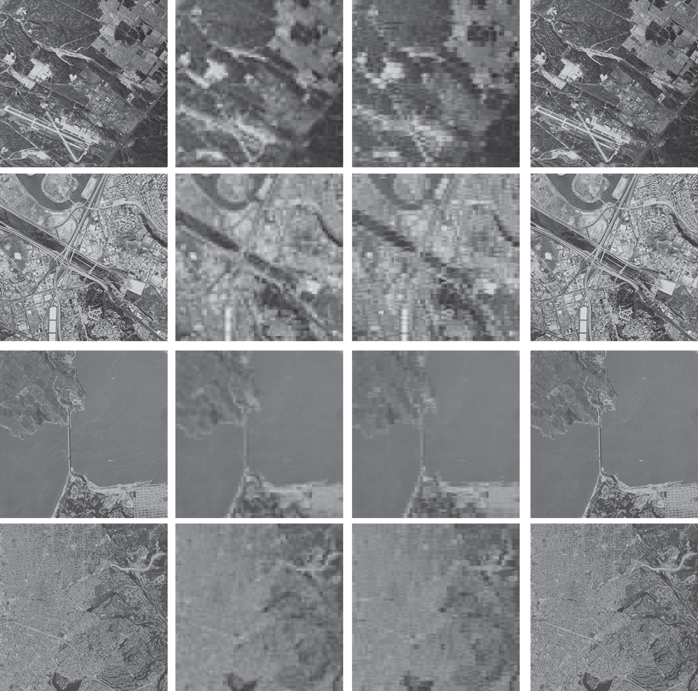
The first four reconstruction images of the aerials volume of USC-SIPI image database from left to right: original image, reconstruction image of DCT, reconstruction image of SR, reconstruction image of the proposed method.

Fig.4

The first four reconstruction images of the miscellaneous volume of USC-SIPI image database from left to right: original image, reconstruction image of DCT, reconstruction image of SR, reconstruction image of the proposed method.

Fig.5

The first four reconstruction images of the textures volume of USC-SIPI image database from left to right: original image, reconstruction image of DCT, reconstruction image of SR, reconstruction image of the proposed method.

It is indicated by the experimental results that, if the training samples and testing samples are very similar, even the same, the proposed method can reach excellent reconstruction performance. It can also be discovered by the experimental results that, DCT surpasses SR in reconstruction performance. This may be due to the fact that, the implementation of DCT is not based on a trained DCT dictionary but on the direct DCT. SR is image patch set oriented and is the optimal solution to a set of image patches, hence more sparse coefficients may be needed to recover a given image patch. Inversely, DCT is image patch oriented and is the best solution to a given image patch, thus fewer DCT coefficients may be required to reconstruct theimage patch.

The major weakness of the experiment of image reconstruction is that, the training and testing sample sets are the same. On the one hand, the experimental results of image reconstruction reflect the recovery capability of the proposed method to some extent. On the other hand, the following experiment of video reconstruction employs different training and testing sample sets and can further prove the performance of the proposed method. Another shortcoming of the proposed method is that, the performance promotion is at the expense of huge computation load. However, the proposed method can be exploited by a non-real-time system, which needs high reconstruction performance.

Therefore, in the situation of same training and testing samples, the proposed method achieves perfect reconstruction performance with 2D or 3D LD ISOMAP representations.

4.3 Experiment of video reconstruction

The experiment of video reconstruction is designed to testify the performance of the proposed method with different training and testing samples. The first frame of a video is employed as the training samples, and the second frame of the video is adopted as the testing samples.

The experimental results of the sequences volume of USC-SIPI image database is enumerated in Table 5, and the experimental results of subset D of the HEVC testing sequences is listed in Table 6. It is shown in Tables 5 and 6 that, the proposed method overmatches DCT and SR in reconstruction performance in the case of 2D and 3D LD low representations. The average PSNRs of USC-SIPI sequences are lower than those of HEVC sequences. This is owing to the fact that, USC-SIPI sequences possess more details than HEVC sequences.

Table 5
The experimental results of the sequences volume of USC-SIPI image database

Video PSNR (dB)

1D 2D 3D

DCT SR Proposed DCT SR Proposed DCT SR Proposed

6.1.02 22.5520 22.2118 19.2048 24.7794 24.1787 26.1295 28.6691 28.2660 32.9458

6.2.02 21.7788 21.3828 18.2066 22.4650 22.3565 23.0409 23.9669 23.8677 24.6117

6.3.02 20.7973 20.1041 17.3209 21.2605 21.0328 22.0349 22.7695 22.6777 25.1887

motion02 27.4865 27.3990 24.2777 27.8809 27.7389 30.6940 30.7865 30.1617 35.2667

Average 23.1537 22.7744 19.7525 24.0965 23.8267 25.4748 26.5480 26.2433 29.5032

Video	PSNR (dB)
6.1.02	22.5520	22.2118	19.2048	24.7794	24.1787	26.1295	28.6691	28.2660	32.9458
6.2.02	21.7788	21.3828	18.2066	22.4650	22.3565	23.0409	23.9669	23.8677	24.6117
6.3.02	20.7973	20.1041	17.3209	21.2605	21.0328	22.0349	22.7695	22.6777	25.1887
motion02	27.4865	27.3990	24.2777	27.8809	27.7389	30.6940	30.7865	30.1617	35.2667
Average	23.1537	22.7744	19.7525	24.0965	23.8267	25.4748	26.5480	26.2433	29.5032

Table 6

The experimental results of subset D of the HEVC testing sequences

Video	PSNR (dB)
	1D			2D			3D
	DCT	SR	Proposed	DCT	SR	Proposed	DCT	SR	Proposed
BasketballPass	24.1969	23.6037	20.9477	25.3294	25.2488	25.7756	26.5562	25.9993	30.8714
BlowingBubbles	22.9074	21.9618	19.3791	24.1142	24.0896	24.4915	25.0259	24.6886	29.8451
BQSquare	17.5446	17.2703	16.1523	18.4825	18.0921	20.6833	19.6127	18.7532	31.7384
Flowervase	28.9026	28.5861	25.8904	29.5711	28.7340	32.2940	31.1962	31.0757	45.8287
RaceHorses	20.7119	20.5837	18.2943	22.0495	22.0351	22.2042	23.4721	23.3902	24.5904
Keiba	20.1673	19.7583	17.0495	20.4246	20.1477	22.8813	23.3422	23.0745	28.9733
Mobisode2	34.6645	32.7504	31.0583	38.3330	37.9365	38.4556	39.5598	39.4912	39.6949
Average	24.1565	23.5020	21.2531	25.4720	25.1834	26.6836	26.9664	26.6390	33.0775

The reconstruction frames of Tables 5 and 6 in the situation of 3D LD representations are respectively illustrated in Figs. 6 and 7, where the proposed method holds higher reconstruction performance than DCT and SR.

Fig.6

The reconstruction frames of the sequences volume of USC-SIPI image database from left to right: original frame, reconstruction frame of DCT, reconstruction frame of SR, reconstruction frame of the proposed method.

Fig.7

The reconstruction frames of subset D of the HEVC testing sequences from left to right: original frame, reconstruction frame of DCT, reconstruction frame of SR, reconstruction frame of the proposed method.

Table 7

The experimental results of the records in the Apnea-ECG Database

ECG Signal	Average RMSE
	1D			2D			3D
	DCT	SR	Proposed	DCT	SR	Proposed	DCT	SR	Proposed
a01	0.2602	0.2390	0.3183	0.2588	0.2529	0.2141	0.2565	0.2678	0.2063
a02	0.1383	0.1398	0.1716	0.1358	0.1398	0.1206	0.1296	0.1440	0.1075
a03	0.4213	0.2602	1.0032	0.4182	0.2504	0.2883	0.4141	0.2502	0.2406
a04	0.3829	0.3628	0.5139	0.3783	0.3744	0.3850	0.3741	0.3887	0.2851
a05	0.4472	0.4611	0.5167	0.4447	0.5013	0.2476	0.4427	0.5251	0.2186
a06	0.1531	0.1204	0.2035	0.1509	0.1219	0.1397	0.1476	0.1225	0.1155
a07	0.5595	0.5272	0.7345	0.5546	0.5769	0.5067	0.5459	0.6068	0.4263
a08	0.5769	0.6604	0.7064	0.5756	0.7094	0.4060	0.5709	0.7362	0.3186
a09	0.2000	0.3271	0.2309	0.1964	0.3346	0.1196	0.1929	0.3652	0.0872
a10	0.2776	0.3393	0.3333	0.2738	0.3767	0.2014	0.2708	0.3970	0.1864
a11	0.3007	0.2750	0.3494	0.2970	0.2875	0.1692	0.2896	0.2985	0.1619
a12	0.1117	0.0995	0.1581	0.1099	0.0958	0.1312	0.1066	0.0952	0.0974
a13	0.5053	0.5722	0.9329	0.5013	0.6200	0.6634	0.4978	0.6489	0.4522
a14	0.2439	0.3097	0.2760	0.2387	0.3430	0.1987	0.2338	0.3616	0.1846
a15	0.5260	0.8629	0.9133	0.4766	0.9297	0.7480	0.4621	0.9425	0.6892
a16	0.6776	1.2574	1.0660	0.6637	1.3599	0.7907	0.6500	1.4437	0.5326
a17	0.3767	0.5992	0.4719	0.3717	0.6663	0.2957	0.3579	0.7113	0.2143
a18	0.2026	0.2694	0.2299	0.1997	0.2919	0.1085	0.1961	0.3141	0.1040
a19	0.5946	0.8782	0.8443	0.5882	0.9258	0.7065	0.5767	0.9724	0.5172
a20	0.1538	0.3187	0.3118	0.1483	0.3532	0.2221	0.1454	0.3606	0.1586
Average	0.3555	0.4440	0.5143	0.3491	0.4756	0.3332	0.3431	0.4976	0.2652

It is obvious in the experimental results that, the average PSNRs of the image reconstruction outbalance those of video reconstruction. This is because of the similarities of the former between training and testing samples is better than those of the latter.

Hence, the proposed method can gain satisfied performance of video reconstruction with different training and testing samples.

4.4 Experiment of signal reconstruction

The experimental results of ECG signal reconstruction are illustrated in Table 7. The root of mean square error (RMSE) substitutes for PSNR as the performance metric. It is reflected in Table 7 that, in the case of 2D and 3D representations, the proposed method possesses the least average RMSEs. Thus, the proposed method outbalances the state-of-the-art methods, such as DCT and SR, in the reestablishment capability of 1D ECG signal. This is due to the fact that, ECG signal is periodic and there are many similarities between different chips. It is also revealed in Table 7 that, 1D SR representation overmatches 2D and 3D SR representations in rebuilding ability of ECG signal. This is owing to the fact that, a testing sample owns a nearest neighbor, which is proportional to an atom in the SR training dictionary.

The experimental results of ECG signal reconstruction are also shown in Fig. 8. Only the reconstruction signals of 3D representation in the first cycle of record a09 are displayed. It is further disclosed in Fig. 8 that, the proposed method is superior to DCT and SR in recovery quality of ECG signal.

Fig.8

The reconstruction signals of 3D representation in the first cycle of record a09. Black curve with cross mark is the original signal, red curve with star mark is the recovery signal of the proposed method, green curve with circle mark is the recovery signal of DCT, and the blue curve with square mark is the recovery signal of SR.

5 Conclusions

This paper discusses the inverse problem of ISOMAP and its applications in data reconstruction. The theoretical framework of the proposed method includes four parts: the classical ISOMAP algorithm, the general ISOMAP embedding algorithm, the sparse dictionary learning algorithm, and the sparse ISOMAP reconstruction algorithm. The sparse reconstruction algorithm is a minimization problem based on the sparse priors of the HD data, and is resolved by the conventional ADMM method. It is testified by the experimental results of image, video and signal reconstruction that, the proposed method is superior to the traditional DCT and SR methods in the reconstruction performance of image, video and signal data, in the situation of very LD representations. It is also verified by the experimental results that, the proposed method is especially suitable for the situation that the training and testing samples are very similar. It is further indicated by the experimental results that, the proposed method is very fit for the reconstruction of texture images, which holds plenty of similar image patches.

In our future work, deep learning priors of HD data will be utilized to resolve the inverse problem of ISOMAP, and the out-of-sample extensions of ISOMAP will also be studied.

References

Zhang ,

Ren ,

Liu ,

Xu ,

Guo and

Liu , A survey on emerging computing paradigms for big data, Chinese Journal of Electronics 26(1) (2017), 1–12.

Feng ,

Wei and

B.T.

Megersa , Big scholarly data: A survey, IEEE Transactions on Big Data 3(1) (2017), 18–35.

Spyros , The forthcoming artificial intelligence (AI) revolution: Its impact on society and firms, Futures 90 (2017), 46–60.

Max , Life 3.0: Being human in the age of artificial intelligence, New York, Knopf., ISBN 9781101946596, OCLC 973137375, 2017.

Chao and

Hou-Duo , Convex optimization learning of faithful Euclidean distance representations in nonlinear dimensionality reduction, Mathematical Programming 164(1-2) (2017), 341–381.

Monnig Nathan ,

Bengt and

Meyer Francois , Inverting nonlinear dimensionality reduction with scale-free radial basis function interpolation, Applied and Computational Harmonic Analysis 37(1) (2014), 162–170.

Maoguo ,

Xiangming and

Hao , Optimization methods for regularization-based ill-posed problems: A survey and a multi-objective framework, Frontiers of Computer Science 11(3) (2017), 362–391.

J.B.

Tenenbaum ,

de Silva and

J.C.

Langford , A global geometric framework for nonlinear dimensionality reduction, Science 290(5500) (2000), 2319–2323.

M.V.

Afonso ,

J.M.

Bioucas-Dias and

A.T.

Mário , Figueiredo, Fast image recovery using variable splitting and constrained optimization, IEEE Transactions on Image Processing 19(9) (2010), 2345–2356.

10.

Li and

Trocan , Sparse solution to inverse problem of nonlinear dimensionality reduction, The 11th International Conference on Multimedia and Network Information System (MISSI 2018), Wroclaw, Poland, 2018, pp. 322–331.

11.

Yan ,

Zhao and

Qin , Semi-supervised local multi-manifold Isomap by linear embedding for feature extraction, Pattern Recognition 76 (2018), 662–678.

12.

Hao ,

Baoqun and

Yu , Robust L-isomap with a novel landmark selection method, Mathematical Problems in Engineering (2017), Article Number: 3930957.

13.

Taiguo and

Zixing , An improved Isomap method for manifold learning, International Journal of Intelligent Computing and Cybernetics 10(1) (2017), 30–40.

14.

Bo ,

Ming and

Yupei , A, Pattern Recognition 55 (2016), 215–230.

15.

Dong ,

Chen and

Zongben , Enhancing both efficiency and representational capability of isomap by extensive landmark selection, Mathematical Problems in Engineering (2015), Article Number: 241436.

16.

Qingchao ,

Yingfeng and

Haobin , Traffic state prediction using ISOMAP manifold learning, Physica A - Statistical Mechanics and Its Applications 506 (2018), 532–541.

17.

Kang-Kang ,

Han-Xiong and

Zhen , ISOMAP-based spatiotemporal modeling for lithium-ion battery thermal process, IEEE Transactions on Industrial Informatics 14(2) (2018), 569–577.

18.

Ganvir and

T.I.

Eldho , Watershed classification using isomap technique and hydrometeorological attributes, Journal of Hydrologic Engineering 22(10) (2017), Article Number: 04017040.

19.

Ming-Ai ,

Wei and

Hai-Na , Adaptive feature extraction of motor imagery EEG with optimal wavelet packets and SE-isomap, Applied Sciences-Basel 7(4) (2017), Article Number: 390.

20.

Jyoti ,

Shekhar and

K.P.

Singh , Wireless sensor networks localization using progressive isomap, Wireless Personal Communications 92(3) (2017), 1281–1302.

21.

Fatih ,

Yakhno Valery and

Roland , A survey on inverse problems for applied sciences, Mathematical Problems in Engineering 2013 (2013), 1–19. Article Number: 976837.

22.

Shujun ,

Jianxin and

Hongqing , MRI reconstruction via enhanced group sparsity and nonconvex regularization, Neurocomputing 272 (2018), 108–121.

23.

Jie ,

Bin and

Ying , A survey on compressed sensing in vehicular infotainment systems, IEEE Communications Surveys and Tutorials 19(4) (2017), 2662–2680.

24.

Z.X.

Yuan and

Xiaoqiang , Hyperspectral image superresolution by transfer learning, IEEE Journal of Selected Topics in Applied Earth Observations and Remote Sensing 10(5) (2017), 1963–1974.

25.

Luo ,

Yu and

Wang , An image reconstruction method based on total variation and wavelet tight frame for limited-angle CT, IEEE Access 6 (2018), 1461–1470.

26.

Zhang ,

Xu ,

Yang ,

Li and

Zhang , A Survey of sparse representation: Algorithms and applications, IEEE Access 3 (2015), 490–530.

27.

K.N.

Kishore and

Schneider , Literature survey on low rank approximation of matrices, Linear & Multilinear Algebra 65(11) (2017), 2212–2244.

28.

Liu ,

Ma ,

Rui and

Lu , Locality constrained dictionary learning for non-linear dimensionality reduction and classification, IET Computer Vision 11(1) (2017), 60–67.

29.

A.G.

Christodoulou ,

Zhang ,

Zhao ,

Kevin Hitchens ,

Ho and

Z.-P.

Liang , High-resolution cardiovascular MRI by integrating parallel imaging with low-rank and sparse modeling, IEEE Transactions on Biomedical Engineering 60(11) (2013), 3083–3092.

30.

Lu ,

Xiong ,

Zhang ,

Wang and

Lu , Robust face super-resolution via locality-constrained low-rank representation, IEEE Access 5 (2017), 13103–13117.

31.

Cheng-Zhi ,

Wei and

Pan , Infrared image super-resolution via locality-constrained group sparse model, Acta Physica Sinica 63(4) (2014), Article Number: 044202.

32.

G.J.

Sullivan ,

J.-R.

Ohm ,

W.-J.

Han and

Wiegand , Overview of the high efficiency video Coding (HEVC) standard, IEEE Transactions on Circuits and Systems for Video Technology 22(12) (2012), 1649–1668.

33.

Penzel ,

G.B.

Moody ,

R.G.

Mark ,

A.L.

Goldberger and

J.H.

Peter , The Apnea-ECG database, Computers in Cardiology 27 (2000), 255–258.

34.

A.L.

Goldberger ,

L.A.N.

Amaral ,

Glass ,

J.M.

Hausdorff ,

PCh.

Ivanov ,

R.G.

Mark ,

J.E.

Mietus ,

G.B.

Moody ,

C.-K.

Peng and

H.E.

Stanley , PhysioBank, PhysioToolkit, and PhysioNet: Components of a new research resource for complex physiologic signals, Circulation 101(23) (2000), e215–e220.

35.

Aharon ,

Elad and

Bruckstein , K-SVD: An algorithm for designing overcomplete dictionaries for sparse representation, IEEE Transactions on Signal Processing 54(11) (2006), 4311–4322.

36.

Jain Anil , Fundamentals of digital image processing, 1st edition, Prentice Hall, Englewood Cliffs, NJ, 1989, pp. 150–153.