
Abstract
Time to failure in the lifetime experiments, common that units or individuals are failure with more than one caused of failure defined by competing risks problem. In this paper, we consider the problem of competing risks model when the failure time of units or individuals have Nadarajaha and Haghighi lifetime distribution [1] based on type-II censoring schemes. The point and interval estimates of model parameters are discussed with maximum likelihood and Bayes methods. In Bayesian approach, the MCMC method is employed. The theoretical results are discussed through real life data analysis and simulation study. Finally, we discussed the numerical results in some brief comments.
Keywords
Introduction
Censoring is common phenomenon in life test experiments due to time and cost restrictions in data collection. Ones of the oldest and most widely used type of censoring called type-I and type-II censoring schemes. In both types, censoring scheme does not allow the removal units of the test other than the final termination point. In type-I censoring, number of failure units is random and test time is fixed. But, in type-II censoring scheme failure units is prefixed number and the test time is random. For the possibility of removal units during the test, the two types of censoring scheme is generalized by progressive censoring scheme. The censoring schemes specially, progressive censoring schemes studying in the book of Balakrishnan and Aggarwala [2]. In this article, we are adopted the type-II censoring scheme in discussing the failure time of units under the test when units is failure with more than on case of failure which known with the competing risk problem.
In different area of reliability studying or life testing experiment, the commonly problem is units failure with more than one causes of failure. In these situation, measuring the effect one of the causes respected to the other causes which defined by competing risk problem. This problem is discussed with different author, for exponential lifetime product Cox [3] and for exponential life product under accelerate life tests Balakrishnan and Han [5]. Early, different properties of competing risk model discussed in Crowder [4] discussed under accelerate life test model in Ganguly and Kundu [6], Hanaa Abu-Zinadah and Neveen Ahmed [7]. The problem of the competing risk model is discussed with two different risks under type-II censoring scheme.
Let n independent units are put on a life test, and prior the experiment the integer m is considered, then the first failure T1;m and its caused of failure ρ1 are recorded. The second failure T2;m and its caused of failure ρ2 are recorded and the experiment is continued until m-th failure Tm;m and its caused ρm where ρ i ∈ {1, 2} , i = 1, 2, . . . , m is recorded. The data (T1;m, ρ1)< (T2;m, ρ2)< ⋯< (Tm;m, ρ m ) , is called type-II competing risk data.
The joint likelihood function under observed type-II competing risk sample
Developing estimation procedures of parameters of Nadarajaha and Haghighi lifetime distributions of type-II competing risk data is the main objective of this article. The classical maximum likelihood method as well as Baysian MCMC method are used to compute the point and interval estimates of model parameters. All theoretical results are assessed and compared trough the two, real data set and Monte Carlo simulation.
The paper is organized as follows, The model notations and descriptions discussed in Section 2. The point and approximate intervals under maximum likelihood estimation in Section 3. The MCMC method of Bayesian approach discussed in section 4. In Section 5, theoretical results discussed through real data set. In Section 6, the different methods are compared by conducting Monte Carlo simulations study. Finally, the numerical results discussed through some brief comments in Section 7.
For consideration only two causes of failure some notations are employed to use in this paper
NHD Nadarajaha and Haghighi distribution.
HF Hazard failure rate function.
RF Relability function.
SEL Squard error loss.
MCMC Markov chain Monte Carlo.
MH Metropolis–Hastings.
RMM Radiation male mice.
pdf Probability density function
cdf Cumulative distribution function
HPD Highest credible intervals
GD Gaussian distribution
CI Cofidence interval
ACI Approximate confidence interval
T i Lifetime of the i-th unit.
T ij Lifetime of the i-th unit under cause j, j = 1, 2.
F (.) Cumulative distribution function (cdf) of T i .
f (.) Probability density function (pdf) of T i .
F j (.) cdf of T ij .
f j (.) pdf of T ij .
S
j
(.) Survival function of
ρ i Indicator variable denoting the cause of failure of the i-th unit. Ω j The integer set of failure units under cause j
To simplify the notation we will use henceforth T
i
instead of Ti;m, i = 1, 2, ⋯ , m. The model studied in the paper satisfies the following assumptions Under the time T
ij
which the unit number i is failed due to cause j the lifetime of unit is defined by T
i
= min {Ti1, Ti2}, i = 1, 2, ⋯ , m. The lifetime random variable T
ij
is distributed with Nadarajaha and Haghighi [1] distribution (NHD) function with shape parameters θ and scale parameters β
j
, j = 1, 2 and i = 1, 2, ⋯ , m. Hence, all pdf and cdf of NHD under random variable T
ij
, j = 1, 2, for each i = 1, 2, ⋯ , m, are given by
The NHD is introduced by Nadarajaha and Haghighi [1] as an extension of the exponential one to present a distribution equivalent to the Weibull and gamma. The NHD with parameters (β, θ), is agreer with the Weibull, gamma and the exponentiated exponential distributions. The NHD has closed form RF and HF like the Weibull and the exponentiated exponential distributions, also reduced to the exponential distribution for the value of θ = 1 and it has the zero mode. Hence, NHD has increasing, decreasing or constant HF and more properties of NHD is presented by Nadarajaha and Haghighi [1]. Different method of estimation of NHD is discussed by Dey et al. [13] and for recurrence relations under record statistic Kumar and Dey [14]. The NHD has the property that HF is monotonically increasing or decreasing which doesn’t existed in the Weibull, Gamma or exponentiated exponential distributions. Also, when modeling the data that has mode fixed at zero the NHD is suitable than Weibull, Gamma or exponentiated exponential distributions.
The point MLEs
For the competing risk data T ij from the NHD with parameters (θ, β j ) for j = 1, 2 and i = 1, 2, . . . , m and distribution function given by equations (3) and (4) the joint likelihood function in (1), without normalized constant is reduced to
where Ω j denoted to integer set of index data failed by the case j . Hence, the log-likelihood function written as follows,
The second partially derivatives of the log-likelihood equation (8) is calculated and presented as follows
Under classical estimation discussed in previous section the model parameters are considered as the constant values but in Bayesian approach it is considered as the random variables. So, in this section, the posterior distribution from the model parameters is constructed and the point and the corresponding credible interval is discussed with the help of MCMC method. The prior distribution of parameters (θ, β1, β2) is considered to be independent gamma density given by
methodologies of MCMC are used in different branches of science such as in quantum system see Wang et al. [16]. Hence, different type of MCMC approach are available, the important one called Gibbs sampling and more general Metropolis-within-Gibbs samplers. The important technique which employed in this section to approximate the Bayes estimates is called important sample method. The posterior density function defined in (27) can be written as
Hence, the Bayes estimate in equation (28) is written by
The plot of the two function Let κ = 1 and M =burn-in, to began with initial iteration with maximum likelihood estimates The value θ(κ) is generated from gamma density The two values Put κ = 2 and repeat steps 2 and 3 to obtain the data The Bayes estimate of any function Also the posterior variance of
[Step 1.] The MCMC sample of parameters vector
[Step 2.] Sort (Z l , i = 1, 2, . . . , N - M) to obtain the ordered values, Z(1) < Z(2) < . . . < Z(N-M) .
[Step 3.] Compute the weighted function η
i
[Step 4.] Estimate the γ the quantile of the marginal posterior of η by
[Step 5.] Compute the 100 (1 - α %) credible intervals of θ
[Step 6.] The 100 (1-α%) HPD interval of is the one, with the smallest interval width among all credible intervals.
In this section, we analyze the real data set presented in Hoel [17] which it is obtained from laboratory experiment for the life of male mice at age of 5-6 weeks received a radiation dose of 300 roentgens. The two causes of failure are chosen, reticulum cell sarcoma and thymic Lymphoma. Our purpose is analysis the two causes of death then, we adopted thymic lymphoma to be cause 1 but the cause 2 is consider be reticulum cell sarcoma. The data of 99 radiation failuremice (RFM) is presented in Table 1. The last data is analyzed with different authors, Sarhan et al. [18], Cramer and Schmiedt [19] and Bakoban and Abd-Elmougod [20]. Hence. the type-II competing risks data under consideration two cause of failure thymic lymphoma and reticulum cell sarcoma and the value of m failure taken to be 35 listed in Table 1 and for computational ease, it divided each sample with 1000. Based on the observed data in Table 2, the MLE and the approximate confidence intervals are presented in Table 3. For Bayesian approach non-informative prior is applied to reflect vague prior information. The results of Bayes point and HPD intervals are also, presented in Table 2. Figs. (1–6) describe the simulation number of the parameters vector generated under MCMC approach as well as the corresponding histogram. Figs. (1–6), show the sequence of 11,000 simulated values observation can be confirmed by examining the autocorrelation function for this sequence. displays convergence diagnostic plots for to assess whether the Markov chains have converged. Inferences should not be made if the Markov chain has not converged. The trace plot shows that the mean of the Markov chain is constant over the graph and is stabilized. The chain is able to traverse the support of the target distribution, and the mixing is good. The trace plot shows that the Markov chain appears to have reached a stationary distribution. The results described by Figs. (1–6) show that the highly correlated of the importance sampling sequences.

Simulation number of θ generated by MCMC method.
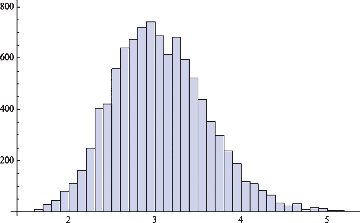
Histogram of θ generated MCMC method.

Simulation number of θ generated by MCMC method.
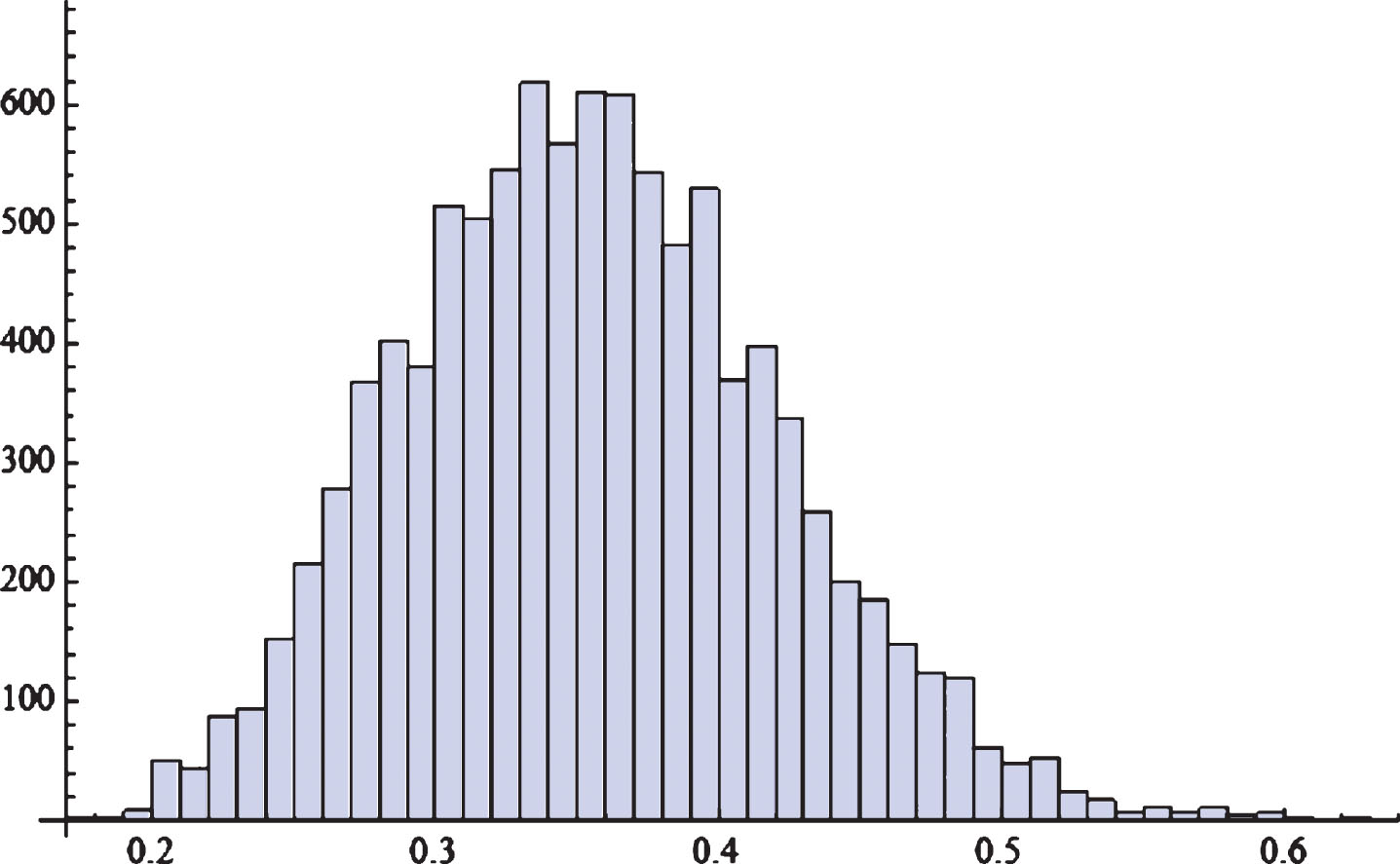
Histogram of θ generated MCMC method.

Simulation number of θ generated by MCMC method.
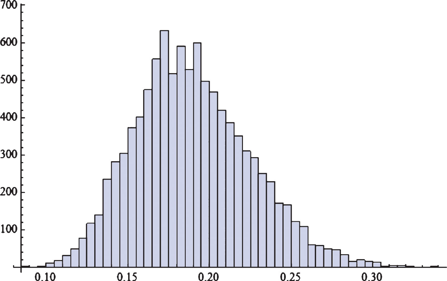
Histogram of θ generated MCMC method.
Hoel [17]
Type-II competing risks data for m = 50
The theoretical results developed in this paper are assessed through observed the behavior of the different proposed methods. Hence simulation study are performed under consideration 1000 type-II competing risks samples. The true values of the model parameters to agreed with hybrid parameters values of prior distribution, we proposed the shape and scale hybrid parameters and generate random sample of size 20. Hence the true parameter is choose to be the mean of the random sample
The point and 95% interval estimates of MLEs and Bayes
The point and 95% interval estimates of MLEs and Bayes
For (θ, β1, β2)= (1.0, 1.5, 2.5), average and mean squared errors (within brackets)
For (θ, β1, β2)=(1.0, 1.5, 2.5), The average 95% confidence lengths and the corresponding coverage percentages
For (θ, β1, β2)= (3.0, 0.5, 1.0), average and mean squared errors (within brackets)
For (θ, β1, β2)=(3.0, 0.5, 1.0), The average 95% confidence lengths and the corresponding coverage percentages
The statistical inference has different applications in more branch of for example in quantum information processing see Batle et al. [21, 22]. This article is dealing with the important problem in life test experiment known with competing risks problem. So, we adopted products has NH lifetime distribution and units is failure with two cause of failure. NHDs with common shape parameter and different scale parameters under type-II censoring scheme is considered. The model parameters are estimated with MLE and Bayes. The inference through real data example also is discussed. We are conducted a simulation study to report the behavior of these estimators. From the results, we observe From Tables 4 to 7, report that estimation procedure discussed in this article is acceptable. The results of the point estimates in Table 4 and 6 show that the Bayes estimators perform better than the MLEs in the terms of MSEs. The results of the interval estimates in Table 5 and 7 show that the Bayes estimators perform better than the MLEs in the terms of mean length and probability coverage. Increasing the sample proportion
Footnotes
Acknowledgement
This project was funded by the Deanship of Scientific Research (DSR) at King Abdulaziz University, Jeddah, under grant no. (KEP-35-130-39). The authors, therefore, acknowledge with thanks DSR for technical and financial support.