Intelligent statistical analysis on the influence of industrial agglomeration on innovation efficiency by spatial econometric model

Abstract

BP neural network method is provided by the outstanding characteristics of self-learning and non-linearity, and can obtain relatively satisfactory prediction results, which also can be used to forecast innovation output. The neural network toolbox function of Matlab can build a neural network prediction model to predict the innovation output from 2008 to 2017. Second, the dynamic SDM is used to empirically test the role of industrial cluster on the innovation efficiency and its space spillover effect by using of the panel data of Chinese cities. The results show the error comparison between the predicted value and real value of innovation efficiency, which explains the accuracy of BP neural network is higher. There is a spatial distribution pattern in which the innovation efficiency decreases from the east, the middle, and the west, which also has the characteristic of time inertia and positive spatial correlation. The producer service agglomeration has significantly improved the innovation efficiency in this city but has no significant role on the innovation efficiency in neighboring cities. The manufacturing cluster has a significant negative effect on the innovation efficiency in this city in the long and short term but produces a significant positive effect on innovation efficiency in neighboring cities in the long and short term.

Keywords

Industrial agglomeration innovation efficiency BP neural network spatial econometric model

1 Introduction

At present, China urgently needs industrial transformation, and the essence of industrial transformation is to improve the innovation efficiency (IE) of industrial enterprises, mainly driven by innovation and energy conservation and emission reduction. Existing research has been carried out at the provincial level to compare the differences in innovation efficiency between different provinces and the influencing factors behind them [1 –3], but the potential important factor of industrial agglomeration has not yet attracted enough attention. The flow of factors and the division of industrial chain between different regions make the investment, production, R&D, and sales links separate and centralize in space, and there will be complex cooperation and competition between companies, which may affect the innovation atmosphere and Innovation performance. Therefore, it is of great research value to investigate the role of industrial agglomeration on the innovation efficiency of industrial enterprises.

2 Related work

At present, domestic and foreign studies on the relationship between industrial cluster and innovation have achieved certain results. Some studies suggested that industrial agglomeration could promote the information exchange and personnel flow in the agglomeration area through the effects of labor pools, technology diffusion, and personnel mobility, thereby accelerating the spillover and diffusion of technology in the agglomeration area, and the technology spillover will help accelerate the technological innovation of enterprises [4]. Krugman [5] believed that industrial agglomeration could increase technology trade in the agglomeration area, and technology trade could boost technological innovation activities and efficiency in the cluster area. Freeman [6] believed that industrial gatherings could ameliorate the investment environment in the cluster area by use of external effects and increased technological innovation activities in the agglomeration area. In terms of empirical research, Storper et al. [7] believed that industrial agglomeration could produce knowledge spillover effect, which was the fundamental driving force for the development of cluster innovation. Andersson et al. [8] used Swedish patent data to verify that industrial agglomeration could significantly promote innovation. Xie et al. [9] believed that the appropriate concentration of industries could improve the efficiency of technological innovation in enterprises through various mechanisms such as learning effects, knowledge spillover effects, economies of scale, competition effects, and cooperation effects. Zhang et al. [10] believed that industrial agglomeration affected the efficiency of technological innovation in industries, and that there were obvious regional differences in the effects.

In summary, this article takes the Chinese 251 cities as the research samples from 2008 to 2017 to explore the following points: (1) Exploring the prediction effect of neural network on innovation output and its role on innovation efficiency. (2) Exploring the relation between industrial cluster and innovation efficiency based on two perspectives of productive services and manufacturing. With the gradual transformation of China’s industry from manufacturing to producer service, the producer service industry has been separated from the traditional industry and developed rapidly, which has formed spatial agglomeration due to the characteristics of high industrial relevance and strong cross-border service. (3) Investigating whether the impact of cluster of producer services and manufacturing on the innovation efficiency of industrial enterprises can spill over to neighboring areas, that is, whether there is a significant space spillover effect. (4) Selecting urban data that better reflects the true level of industrial agglomeration and innovation efficiency as the research samples, rather than provincial data with large spatial scales and internal differences.

3 Empirical research model

3.1 Sample data and variable selection

After deleting cities with severe data missing, this paper selects the input and output data of 251 cities in China. The time span is from 2008 to 2017. The data mainly comes from China City Statistical Yearbook. The specific descriptions of the variables and their calculations are as follows:

Innovation efficiency. This article uses the DEA-BCC model to calculate the innovation efficiency of industrial companies, and selects the proportion of technical service employees, R&D funding stock, new product development funding stock and industrial electricity as input indicators, and uses the number of invention patent applications as output indicators.

Industrial agglomeration level. This article uses location entropy index to calculate the levels of producer service agglomeration (SA) and manufacturing agglomeration (MA). This article selects the proportion of the number of employees in the producer service industry or manufacturing industry in each city to the number of employees in the region / the ratio of the number of employees in producer services or manufacturing industry to the number of employees in the country: ${Aggl}_{ij} = \frac{E_{ij} / E_{i}}{E_{j} / E}$ (1)

Where E_ij is the employees number of j industry in i city, E_i is the number of employees in all industries in i city, E_j s the number of employees in j industry in all cities, E is the total number of employees.

Control variables. 1) Industrial Structure (IND), which is expressed by the increase of the tertiary industry as a percentage of GDP. 2) Innovation environment (INV), which is expressed by the proportion of the number of industrial companies conducting R&D activities to the total number of industrial enterprises. 3) Foreign direct investment (FDI), which is expressed by the actual use of foreign investment as a percentage of GDP. 4) Human capital level (HC), which is expressed by the number of college graduates and above per 100000 population.

3.2 DEA model

DEA method uses the input and output variables of decision unit (DMU), and uses mathematical planning methods to measure the leading edge of the effective DMU, and then analyzes the degree of deviation of each DMU from the leading edge of the production to estimate the relative efficiency of each DMU [11, 12]. CCR model assumes that the scale benefits of production technology remain unchanged. However, in the actual production process, many production units do not reach the optimal scale, so the technical efficiency measured by CCR model includes scale efficiency. In 1984, Banker et al [13] proposed a DEA model for estimating scale efficiency, also known as the BCC model. Supposing there are n DMUs, each of which has m types of inputs and s types of outputs. For a specific DMU, the input-oriented CCR model is: $\begin{matrix} min [θ - ɛ (e^{T} s^{-} + \overset{\land^{T}}{e} s^{+})] \\ \begin{matrix} s . t . \sum_{j = 1}^{n} x_{j} λ_{j} \end{matrix} + s^{-} = θ x_{0} \\ \begin{matrix} \sum_{j = 1}^{n} y_{j} λ_{j} - s^{+} \end{matrix} = y_{0} \\ \begin{matrix} λ_{j} \end{matrix} \geq 0, j = 1, . . ., n . \\ \begin{matrix} s^{+} \end{matrix} \geq 0, s^{-} \geq 0 \end{matrix}$ (2)

The production set corresponding to the above model is: $T = {(x, y) | \begin{matrix} \sum_{j = 1}^{n} x_{j} λ_{j} \leq x, \sum_{j = 1}^{n} y_{j} λ_{j} \leq y, \\ y \geq 0, λ_{j} \geq 0, j = 1, . . ., n . \end{matrix}}$ (3)

The input-oriented BCC model is as follows: $\begin{matrix} min [θ - ɛ (e^{T} s^{-} + \overset{\land^{T}}{e} s^{+})] \\ \begin{matrix} s . t . \sum_{j = 1}^{n} x_{j} λ_{j} \end{matrix} + s^{-} = θ x_{0} \end{matrix}$ $\begin{matrix} \begin{matrix} \sum_{j = 1}^{n} y_{j} λ_{j} - s^{+} \end{matrix} = y_{0} \\ \begin{matrix} \sum_{j = 1}^{n} λ_{j} \end{matrix} = 1 \\ \begin{matrix} λ_{j} \end{matrix} \geq 0, j = 1, . . ., n . \\ \begin{matrix} s^{+} \end{matrix} \geq 0, s^{-} \geq 0 \end{matrix}$ (4)

3.3 Derivation of BP algorithm formula

The basic BP algorithm includes 2 aspects: the forward propagation of the signal and the backward propagation of the error. The actual output is estimated in the direction from input to output, and the correction of weights and thresholds is performed in the direction from output to input in Fig. 1.

Fig. 1

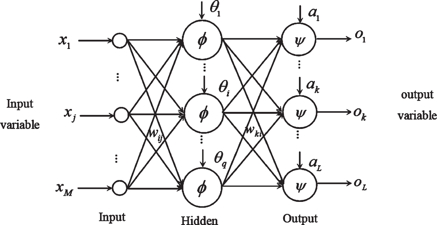
Structure of BP network.

Where x_j represents the input of j node of input layer, j = 1, 2, . . . , M. w_ij represents the weight between the i-th node in the hidden layer and the j-th node in the input layer. θ_i represents the threshold of the i-th node of the hidden layer. ϕ (x) represents the excitation function of the hidden layer. w_ki represents the weight between the first node in the output layer and the i-th node in the hidden layer, i = 1, 2, . . . , q. α_k represents the threshold of the k-th node of the output layer, k = 1, 2, . . . , L. Ψ (x) represents the excitation function of the output layer. o_k represents the output of first node of output layer.

(1) Forward propagation of the signal

Input net_i of the i-th node of the hidden layer: ${net}_{i} = \sum_{j = 1}^{M} w_{ij} x_{j} + θ_{i}$ (5)

The output y_i of the i-th node of the hidden layer: $y_{i} = ϕ ({net}_{i}) = ϕ (\sum_{j = 1}^{M} w_{ij} x_{j} + θ_{i})$ (6)

The input net_i of the k-th node of the output layer: ${net}_{i} = \sum_{i = 1}^{q} w_{ki} y_{i} + α_{k} = \sum_{i = 1}^{q} w_{ki} ϕ (\sum_{j = 1}^{M} w_{ij} x_{j} + θ_{i}) + α_{k}$ (7)

The output ok of the k-th node of the output layer: $\begin{matrix} o_{k} = Ψ ({net}_{i}) = ψ (\sum_{i = 1}^{q} w_{ki} y_{i} + α_{k}) = ψ (\sum_{i = 1}^{q} w_{ki} \\ = ψ (\sum_{i = 1}^{q} w_{ki} ϕ (\sum_{j = 1}^{M} w_{ij} x_{j} + θ_{i}) + α_{k}) \end{matrix}$ (8)

(2) Back propagation process of errors

Back propagation of errors starts from the output layer to calculate the output error of each layer of neurons layer by layer, and then adjusts the weights and thresholds of each layer according to the error gradient descent method, so that the final output of the modified network can approach the expected value.

The quadratic error criterion function for each sample p is E_p: $E_{p} = \frac{1}{2} \sum_{k = 1}^{L} (T_{k} - o_{k})^{2}$ (9) The system’s total error criterion function for P training samples is: $E = \frac{1}{2} \sum_{p = 1}^{P} \sum_{k = 1}^{L} (T_{k}^{p} - o_{k}^{p})^{2}$ (10)

Based on error gradient descent method, the correction amount Δw_ki of the output layer weight, the correction amount Δα_k of the output layer threshold, the correction amount Δw_ij of the hidden layer weight, and the correction amount Δθ_i of the hidden layer threshold are sequentially revised. $\begin{matrix} Δ w_{ki} = - η \frac{\partial E}{\partial w_{ki}}; \\ Δ α_{k} = - η \frac{\partial E}{\partial α_{k}}; \\ Δ w_{ij} = - η \frac{\partial E}{\partial w_{ij}}; \\ Δ θ_{i} = - η \frac{\partial E}{\partial θ_{i}}; \end{matrix}$ (11)

Output layer weight adjustment formula: $\begin{matrix} Δ w_{ki} = - η \frac{\partial E}{\partial w_{ki}} \\ = - η \frac{\partial E}{\partial {net}_{k}} \frac{\partial {net}_{k}}{\partial w_{ki}} \\ = - η \frac{\partial E}{\partial o_{k}} \frac{\partial o_{k}}{\partial {net}_{k}} \frac{\partial {net}_{k}}{\partial w_{ki}} \end{matrix}$ (12)

Output layer threshold adjustment formula: $\begin{matrix} Δ α_{k} = - η \frac{\partial E}{\partial α_{k}} \\ = - η \frac{\partial E}{\partial {net}_{k}} \frac{\partial {net}_{k}}{\partial α_{k}} \\ = - η \frac{\partial E}{\partial o_{k}} \frac{\partial o_{k}}{\partial {net}_{k}} \frac{\partial {net}_{k}}{\partial α_{k}} \end{matrix}$ (13)

Hidden layer weight adjustment formula: $\begin{matrix} Δ w_{ij} = - η \frac{\partial E}{\partial w_{ij}} \\ = - η \frac{\partial E}{\partial {net}_{i}} \frac{\partial {net}_{i}}{\partial w_{ij}} \\ = - η \frac{\partial E}{\partial y_{i}} \frac{\partial y_{i}}{\partial {net}_{i}} \frac{\partial {net}_{i}}{\partial w_{ij}} \end{matrix}$ (14)

Hidden layer threshold adjustment formula: $\begin{matrix} Δ θ_{i} = - η \frac{\partial E}{\partial θ_{i}} \\ = - η \frac{\partial E}{\partial {net}_{i}} \frac{\partial {net}_{i}}{\partial θ_{i}} \\ = - η \frac{\partial E}{\partial y_{i}} \frac{\partial y_{i}}{\partial {net}_{i}} \frac{\partial {net}_{i}}{\partial θ_{i}} \end{matrix}$ (15)

Also due to: $\frac{\partial E}{\partial o_{k}} = - \sum_{p = 1}^{P} \sum_{k = 1}^{L} (T_{k}^{p} - o_{k}^{p})$ (16) $\begin{matrix} \frac{\partial {net}_{k}}{\partial w_{ki}} = y_{i}; \\ \frac{\partial {net}_{k}}{\partial a_{k}} = 1; \\ \frac{\partial {net}_{k}}{\partial w_{ij}} = x_{j}; \\ \frac{\partial {net}_{k}}{\partial θ_{i}} = 1 \end{matrix}$ (17) $\frac{\partial E}{\partial o_{k}} = - \sum_{p = 1}^{P} \sum_{k = 1}^{L} (T_{k}^{p} - o_{k}^{p}) Ψ^{'} ({net}_{k}) w_{ki}$ (18) $\frac{\partial y_{i}}{\partial {net}_{i}} = ϕ^{'} ({net}_{k}) w_{ki}$ (19) $\frac{\partial o_{k}}{\partial {net}_{i}} = ψ^{'} ({net}_{k})$ (20)

So in the end we get the following formula: $Δ w_{ki} = η \sum_{p = 1}^{P} \sum_{k = 1}^{L} (T_{k}^{p} - o_{k}^{p}) Ψ' ({net}_{k}) y_{i}$ (21) $Δ a_{i} = η \sum_{p = 1}^{P} \sum_{k = 1}^{L} (T_{k}^{p} - o_{k}^{p}) Ψ' ({net}_{k})$ (22) $\begin{matrix} Δ w_{ij} = η \sum_{p = 1}^{P} \sum_{k = 1}^{L} (T_{k}^{p} - o_{k}^{p}) \\ Ψ' ({net}_{k}) w_{ki} ϕ' ({net}_{k}) x_{j} \end{matrix}$ (23) $\begin{matrix} Δ θ_{i} = η \sum_{p = 1}^{P} \sum_{k = 1}^{L} (T_{k}^{p} - o_{k}^{p}) \\ Ψ' ({net}_{k}) w_{ki} ϕ' ({net}_{k}) \end{matrix}$ (24)

3.4 Cluster analysis

According to the classification process, it can be divided into three methods: K-means clustering, system clustering, and two-step clustering. The basic idea of systematic cluster analysis is: samples (or variables) that are close to each other are clustered into a class first, and clusters that are far away are clustered into a class. The process continues, and each sample (or variable) can always be clustered into the appropriate class. Before systematic clustering, the distance between classes must be defined. The difference in the definition of distance between classes leads to different systematic clustering methods. Their classification steps are basically the same, but the main difference is the calculation method of the distance between classes.

This paper uses d_ij to represent the distance of sample X_i and X_j, and uses D_ij to represent Z_i and Z_j. This paper uses the center of gravity method to define the distance between classes. Supposing Z_p and Z_qhaven_p and n_q respectively, and there centers of gravity are ${\bar{X}}_{p}$ and ${\bar{X}}_{q}$ respectively, and the distance of Z_p and Z_q is defined as the distance of ${\bar{X}}_{p}$ and ${\bar{X}}_{q}$ . This article uses Euclidean distance to represent as follows: $D_{pq}^{2} = (\bar{X_{p}} - \bar{X_{q}})^{(} \bar{X_{p}} - \bar{X_{q}})$ (25)

Supposing Z_p and Z_q are combined into Z_r, then the sample number of Z_r is n_r = n_p + n_q, and the center of gravity is ${\bar{X}}_{r} = \frac{1}{n_{r}} (n_{p} {\bar{X}}_{p} + n_{q} {\bar{X}}_{q})$ , the center of Z_k is ${\bar{X}}_{k}$ . According to formula (25), the distance from the new class is $D_{kr}^{2} = \frac{n_{p}}{n_{r}} D_{kp}^{2} + \frac{n_{q}}{n_{r}} D_{kq}^{2} - \frac{n_{p} n_{q}}{n_{r}} D_{pq}^{2}$ (26)

In fact, the distance between the class and the new class represented by formula (26) is: $\begin{matrix} D_{kr}^{2} = (\bar{X_{k}} - \bar{X_{r}})^{,} (\bar{X_{k}} - \bar{X_{r}}) \\ = [{\bar{X}}_{k} - \frac{1}{n_{r}} (n_{p} {\bar{X}}_{p} + n_{q} {\bar{X}}_{q})]^{'} \\ [{\bar{X}}_{k} - \frac{1}{n_{r}} (n_{p} {\bar{X}}_{p} + n_{q} {\bar{X}}_{q})] \\ = {\bar{X}}_{k}^{'} {\bar{X}}_{k} - 2 \frac{n_{p}}{n_{r}} {\bar{X}}_{k}^{'} {\bar{X}}_{p} - 2 \frac{n_{p}}{n_{r}} {\bar{X}}_{k}^{'} {\bar{X}}_{q} \\ + \frac{1}{n_{r}^{2}} (n_{p}^{2} {\bar{X}}_{p}^{'} {\bar{X}}_{p} + 2 n_{p} n_{q} {\bar{X}}_{p} {\bar{X}}_{q} \\ - n_{q}^{2} {\bar{X}}_{q}^{'} {\bar{X}}_{q}) \end{matrix}$ (27)

Put ${\bar{X}}_{k}^{'} {\bar{X}}_{k} = \frac{1}{n_{r}} (n_{p} {\bar{X}}_{k}^{'} {\bar{X}}_{k} + n_{q} {\bar{X}}_{k}^{'} {\bar{X}}_{k})$ into the above formula, there are $\begin{matrix} D_{kr}^{2} = (\bar{X_{k}} - \bar{X_{r}})^{(} \bar{X_{k}} - \bar{X_{r}}) \\ = [{\bar{X}}_{k} - \frac{1}{n_{r}} (n_{p} {\bar{X}}_{p} + n_{q} {\bar{X}}_{q})]^{'} \\ [{\bar{X}}_{k} - \frac{1}{n_{r}} (n_{p} {\bar{X}}_{p} + n_{q} {\bar{X}}_{q})] \\ = {\bar{X}}_{k}^{'} {\bar{X}}_{k} - 2 \frac{n_{p}}{n_{r}} {\bar{X}}_{k}^{'} {\bar{X}}_{p} \\ - 2 \frac{n_{p}}{n_{r}} {\bar{X}}_{k}^{'} {\bar{X}}_{q} + \frac{1}{n_{r}^{2}} (n_{p}^{2} {\bar{X}}_{p}^{'} {\bar{X}}_{p} \\ + 2 n_{p} n_{q} {\bar{X}}_{p} {\bar{X}}_{q} - n_{q}^{2} {\bar{X}}_{q}^{'} {\bar{X}}_{q}) \end{matrix}$ (28)

3.5 Spatial autocorrelation test

The Moran’s I index was first presented by Moran in 1948 [14], and its expression is as follows: ${Moran}^{'} sI = \frac{\sum_{i = 1}^{n} \sum_{j = 1}^{n} W_{ij} (X_{i} - \bar{X}) (X_{j} - \bar{X})}{S^{2} \sum_{i = 1}^{n} \sum_{j = 1}^{n} W_{ij}}$ (29)

Where $S^{2} = (1 / n) \sum_{i = 1}^{n} (X_{i} - \bar{X})^{2}$ , $\bar{X} = (1 / n) \sum_{i = 1}^{n} X_{i}$ . Y_i and Y_j are the observations of the i-th city and j-th city. W_ij is the dimensional space weight matrix. The significance level of Moran’s I index can be tested by standardized statistics Z, and its expression is: $Z = \frac{{Moran}^{'} sI - E (I)}{\sqrt{VAR (I)}}$ (30)

3.6 Space weight matrix

(1) Geographic distance weight matrix (W^g). The geographic distance weight matrix is found by using of the inverse of the spherical distance based on the geographic unit, which is specifically expressed as: $W^{e} = {\begin{matrix} \frac{1}{| d_{ij} |}, i \neq j \\ 0, i = j \end{matrix}$ (31)

Where d_ij is the distance between the 2 cities measured by the latitude and longitude data.

(2) Economic distance weight matrix (W^e). Considering that the correlation effects of the mutual influences caused by the differences in economic development between different cities are not the same, this article uses the actual per capita GDP as a measure of the urban economic development level, and constructs a matrix of economic distance weights as follows: $W^{e} = {\begin{matrix} \frac{1}{| {\bar{Q}}_{i} - {\bar{Q}}_{j} |}, i \neq j \\ 0, i = j \end{matrix}$ (32)

Where ${\bar{Q}}_{i}$ and ${\bar{Q}}_{j}$ respectively represent the average of the actual per capita GDP of the two cities during the study period.

3.7 Measurement model setting

Space econometric models mainly include space lag model (SAR) and space error model (SEM) [15]. Lesage et al. [16] proposed a more extensive spatial econometric model than SAR and SEM, taking into account exogenous and endogenous variables of spatial lag, which is the spatial Durbin model (SDM), and the expression is: $\begin{matrix} y_{it} = ρ \sum_{j = 1}^{N} w_{ij} y_{jt} + β x_{it} + θ \sum_{j = 1}^{N} w_{ij} x_{jt} \\ + μ_{i} + v_{t} + ɛ_{it} \end{matrix}$ (33)

Where ρ is the space autoregressive coefficient, β and θ respectively represent the coefficient of the exogenous variable and its space lag term. μ_i and v_t represent regional and time effects, respectively. ɛ_it is random perturbations. The dynamic spatial Durbin model expression is as follows: $\begin{matrix} y_{it} = λ y_{it - 1} + α \sum_{j = 1}^{N} w_{ij} y_{jt - 1} + ρ \sum_{j = 1}^{N} w_{ij} y_{jt} \\ + β x_{it} + θ \sum_{j = 1}^{N} w_{ij} x_{jt} + μ_{i} + v_{t} + ɛ_{it} \end{matrix}$ (34)

Regarding the estimation of the dynamic SDM model, Yu et al. [17] constructed the corrective estimator of dynamic SLM after analyzing the asymptotic properties of their maximum likelihood estimators. The estimation methods of dynamic spatial Durbin model and dynamic SAR model are basically similar. Elhorst [18] believed that the maximum likelihood estimation method with bias correction for estimation had a good small sample property and could solve the bias problem of the ordinary maximum likelihood method.

4 Analysis of empirical results

4.1 Analysis of innovation efficiency

The average value of innovation efficiency from 2008 to 2017 is shown in Table 1. It can be seen that China’s innovation efficiency is on the rise as a whole, with an average annual growth rate of 1.89%, reaching 0.8199 in 2017. The main factors affecting innovation output are the proportion of technical service employees, R&D funding stock, new product development funding stock and industrial electricity as input indicators. Therefore, this paper uses these input indicators to predict the innovation output based on BP neural network. It is easy to discover from Table 1 that the predicted innovation output is brought into the DEA model and new innovation efficiency is obtained. Judging from the prediction results, except for individual years, the prediction error using the BP network is relatively small. Therefore, the prediction effect using the BP neural network is satisfactory. In addition, this article used SPSS22.0 software to perform a systematic clustering analysis on the innovation efficiency of 251 cities in mainland China over the years. All data are divided into innovation efficiency high efficiency area, medium efficiency area, and low efficiency area (limited to space, clustering results are omitted). It can be discovered that, in general, the cities in the area of high innovation efficiency are mainly located in the eastern coastal areas, the cities in the area of medium innovation efficiency are mainly in the central and western regions, and the cities in the area of innovation efficiency are mainly in the western area. This shows that China’s regional innovation efficiency presents certain regional characteristics.

Table 1
Average value of China’s innovation efficiency from 2008 to 2017

Year Actual value Predictive value Relative error/%

2008 0.6939 0.6927 0.162

2009 0.7506 0.7534 0.362

2010 0.7259 0.7242 0.233

2011 0.7248 0.7278 0.414

2012 0.7684 0.7661 0.296

2013 0.7555 0.7571 0.222

2014 0.8256 0.8270 0.173

2015 0.8261 0.8291 0.361

2016 0.8314 0.8327 0.154

2017 0.8199 0.8222 0.285

Year	Actual value	Predictive value	Relative error/%
2008	0.6939	0.6927	0.162
2009	0.7506	0.7534	0.362
2010	0.7259	0.7242	0.233
2011	0.7248	0.7278	0.414
2012	0.7684	0.7661	0.296
2013	0.7555	0.7571	0.222
2014	0.8256	0.8270	0.173
2015	0.8261	0.8291	0.361
2016	0.8314	0.8327	0.154
2017	0.8199	0.8222	0.285

4.2 Space autocorrelation test

Moran’s I index was used to test the space autocorrelation of innovation efficiency (limited in length, the calculation results are omitted). The test results indicate the Moran’s I index passes the significance level test of 1% or 5% from 2008 to 2017, which indicates that the IE of industrial enterprises is not completely random and there is a certain positive spatial correlation. Therefore, it is obliged to carry out a quantitative analysis of the influencing factors of innovation efficiency of industrial enterprises from the spatial dimension. In addition, compared with the geographic distance weight matrix, the Moran statistics under the economic distance weight matrix are generally higher, which means the economic distance characteristics have a greater impact on the spatial correlation of urban innovation efficiency. This further illustrates that cities with similar economic characteristics are more likely to have a spatial interaction effect on innovation efficiency.

4.3 Estimate results and analysis

First, the LM statistic test and Robust LM statistic test are performed on the non-spatial interaction model in four forms. The calculation results are shown in Tables 2-3. it can be discovered that the LR test rejected the null hypothesis at 1% level, indicating the model should include both space and time fixed effects. Consequently, the LM test results must be estimated on the basis of the space and time dual fixed effect model. The LM statistics tests in Tables 2-3 both reject the null hypothesis at a significance level of 1%, indicating that SAR and SEM should be established at the same time, also indicating that the SDM needs to be further estimated. In all the tables below, ***, **, * indicate that they passed the significance test at the levels of 1%, 5%, 10% respectively.

Table 2
Test results of spatial effects under static conditions (geographic distance weight)

Weights Test type Mixed estimation model Spatial fixed effect model time fixed effect model Space-time fixed effect model

W ^g LM spatial lag 20.2441^* 24.5577^* 17.3545^* 14.7419^*

Robust LM spatial lag 10.1760^* 12.7032^* 11.8351^* 11.6361^*

LM spatial error 32.2976^* 19.9762^* 24.7281^* 17.8116^*

Robust LM spatial error 8.0721^* 9.2927^* 7.7797^* 10.0320^*

Spatial fixed effect LR test 421.6452^*

Time fixed effect LR test 216.4643^*

Weights	Test type	Mixed estimation model	Spatial fixed effect model	time fixed effect model	Space-time fixed effect model
W ^g	LM spatial lag	20.2441^***	24.5577^***	17.3545^***	14.7419^***
	Robust LM spatial lag	10.1760^***	12.7032^***	11.8351^***	11.6361^***
	LM spatial error	32.2976^***	19.9762^***	24.7281^***	17.8116^***
	Robust LM spatial error	8.0721^***	9.2927^***	7.7797^***	10.0320^***
	Spatial fixed effect LR test	421.6452^***
	Time fixed effect LR test	216.4643^***

Table 3

Test results of spatial effects under static conditions (economic distance weight)

Weights	Test type	Mixed estimation model	Spatial fixed effect model	time fixed effect model	Space-time fixed effect model
W ^e	LM spatial lag	18.1171^***	32.0052^***	23.6386^***	20.9477^***
	Robust LM spatial lag	11.6203^***	17.2084^***	16.6570^***	13.0815^***
	LM spatial error	33.4821^***	23.9282^***	28.5156^***	26.5484^***
	Robust LM spatial error	8.4897^***	9.3378^***	7.3244^***	10.9944^***
	Spatial fixed effect LR test	486.2465^***
	Time fixed effect LR test	235.1904^***

On account of the above analysis, this article conducted a Ward test and an LR test on the conversion of the static spatial Durbin model into SAR and SEM models. The test results show that the static SDM cannot be degraded into SAR and SEM models. This means that it is more effective to select a more generalized form of SDM model for empirical analysis than SAR and SEM models. In the end, the Hausman test is used to test whether the model chooses a fixed effect or a random effect. The results show that the fixed effect of the dynamic SDM passes the significance test at 1% level. Therefore, this paper chooses the dynamic SDM with fixed effects of space and time. The estimation results are shown in Tables 4-5. In addition, it is found that the coefficient estimates under the economic distance weight are significantly different from the coefficient estimates under the geographic weight matrix.

Table 4

Estimation results of static and dynamic spatial Durbin models (geographic distance weights)

Variables	Static SDM	Dynamic SDM
lnIE_t - 1		0.0347^***
W*lnIE_t - 1		0.0204^***
lnSA	0.0702^**	0.0637^***
lnMA	–0.0252^*	–0.0237^**
lnIND	0.1302	0.1039^*
lnINV	0.0464^*	0.0491^*
lnFDI	0.0073^*	0.0072^**
lnHC	–0.0942	–0.1074
W*lnSA	0.0155	0.0210
W*lnMA	0.0231^*	0.0234^*
W*lnIND	0.0277	0.0249
W*lnINV	0.0270^*	0.0263^*
W*lnFDI	0.0019	0.0054^*
W*lnHC	–0.0120	–0.0128
ρ	0.3102^***	0.3169^***
R-squared	0.6902	0.6992
Log-likelihood	731.5789	750.8179
N	2510	2510

Table 5

Estimation results of static and dynamic spatial Durbin models (economic distance weights)

Variables	Static SDM	Dynamic SDM
lnIEt-1		0.0379^***
W*lnIEt-1		0.0230^***
lnSA	0.0713^***	0.0644^***
lnMA	–0.0256^**	–0.0247^**
lnIND	0.1353^*	0.1045^*
lnINV	0.0566^*	0.0605^*
lnFDI	0.0062^*	0.0082^**
lnHC	–0.0986	–0.1039
W*lnSA	0.0172	0.0223
W*lnMA	0.0285^**	0.0241^**
W*lnIND	0.0219	0.0263
W*lnINV	0.0305^*	0.0222^*
W*lnFDI	0.0047^*	0.0065^*
W*lnHC	–0.0145	–0.0114
ρ	0.3159^***	0.3180^***
R-squared	0.6928	0.7015
Log-likelihood	745.0997	757.1219
N	2510	2510

In order to further explain whether the dynamic SDM will increase the interpretation of the model, this paper uses LR test to analyze the joint significance of IE_t - 1 and W * IE_t - 1. The results show that the LR statistics under both weight matrices pass the 1% level of significance test. It should be pointed out that, whether it is a static SDM or a dynamic SDM, the estimated Log-L value and R² value under economic distance weight are better than that under the geographical distance weight. Therefore, the following analysis focuses on the double-fixed-effect dynamic space Durbin model under the economic distance weight matrix.

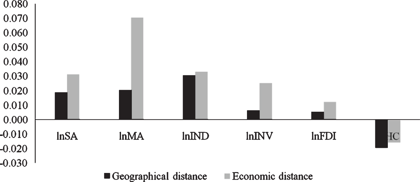
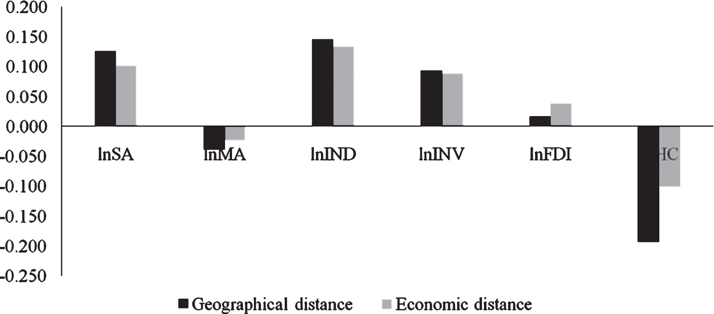
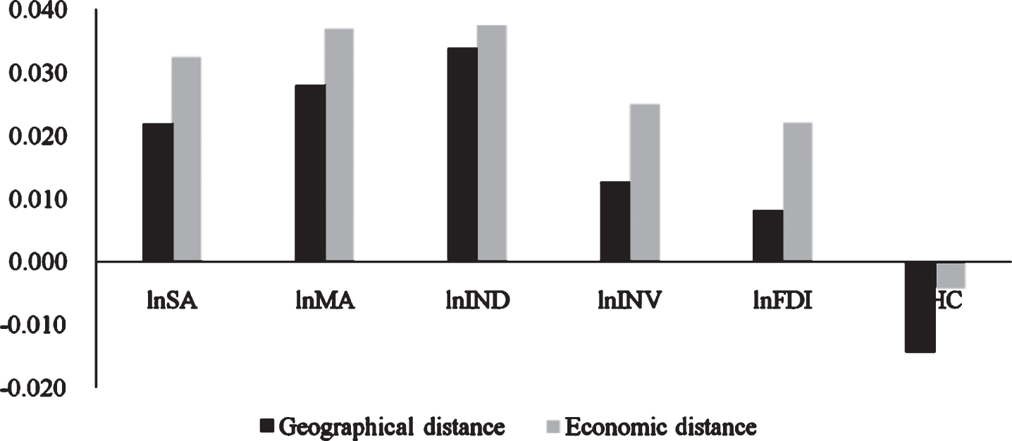
4.4 Direct and indirect effects analysis

The direct and indirect effects are further decomposed into short-term effects and long-term effects in the time dimension to reflect the short-term immediate impact of industrial cluster on innovation efficiency and the long-term impact of considering time lag. The results are shown in Tables 6-7. Figs. 2 –5 show the estimated coefficients of the short-term direct effects, short-term indirect effects, long-term direct effects, and long-term indirect effects under two weights. After comparison, it is found that no matter what kind of effect, the coefficient estimates under the economic distance weight are significant differences in the estimated coefficients under the geographic distance weighting.

Table 6
Effect decomposition of each variable on innovation efficiency (geographic distance weighting)

Variables Short-term direct effect Short-term indirect effect Long-term direct effect Long-term indirect effect

lnSA 0.0664^* 0.0189 0.1256^* 0.0218

lnMA –0.0316^** 0.0205^* –0.0386^ 0.0279^

lnIND 0.0768^* 0.0306 0.1457^* 0.0338

lnINV 0.0424^* 0.0065^* 0.0930^ 0.0126^

lnFDI 0.0079^** 0.0054^* 0.0165^** 0.0081^*

lnHC –0.0995 –0.0194 –0.1932 –0.0144

Variables	Short-term direct effect	Short-term indirect effect	Long-term direct effect	Long-term indirect effect
lnSA	0.0664^***	0.0189	0.1256^***	0.0218
lnMA	–0.0316^**	0.0205^*	–0.0386^**	0.0279^**
lnIND	0.0768^*	0.0306	0.1457^*	0.0338
lnINV	0.0424^*	0.0065^*	0.0930^**	0.0126^**
lnFDI	0.0079^**	0.0054^*	0.0165^**	0.0081^*
lnHC	–0.0995	–0.0194	–0.1932	–0.0144

Table 7

Effect decomposition of each variable on innovation efficiency (economic distance weighting)

Variables	Short-term direct effect	Short-term indirect effect	Long-term direct effect	Long-term indirect effect
lnSA	0.0866^***	0.0314	0.1005^***	0.0323
lnMA	–0.0169^**	0.0704^**	–0.0227^**	0.0367^**
lnIND	0.1082^*	0.0331	0.1326^*	0.0374
lnINV	0.0606^*	0.0253^*	0.0872^***	0.0249^**
lnFDI	0.0320^**	0.0124^*	0.0377^**	0.0220^**
lnHC	–0.0770	–0.0155	–0.0998	–0.0041

Fig. 2

Coefficient estimation of short-term direct effects.

Fig. 3

Coefficient estimation of short-term indirect effects.

Fig. 4

Coefficient estimation of long-term direct effects.

Fig. 5

Coefficient estimation of long-term indirect effects.

According to Tables 6-7, it can be found that, whether in the long or short term, the direct effect of agglomeration of productive service industries is positive, passing the test of 1% level. However, the indirect effect of the of producer service cluster is positive but not significant, which indicates an increase in the level of producer service cluster can significantly improve the innovation efficiency in this city, but it has no significant role in promoting the improvement of innovation efficiency in neighboring cities. The producer service agglomeration can speed up the construction of industrial enterprise innovation platforms, provide technical personnel from different regions and enterprises with opportunities for cooperation and exchange, and help to share first-class skills and managerial experiences in innovation. From the estimation results of manufacturing cluster, manufacturing cluster has a significant inhibitory role on the innovation efficiency of industrial enterprises in this city, but it has a positive role in boosting the innovation efficiency of industrial enterprises in neighboring cities. China’s manufacturing industry mainly relies on industrial parks to agglomerate, mostly horizontal or simple vertical agglomeration, which makes imitative innovation more common, leading to the positive effect of positive knowledge spillovers brought by agglomeration on innovation efficiency. The recent suppression effect surpassed, hindering the promotion of innovation efficiency in the entire agglomeration area. Nevertheless, with the further deepening of the division of labor between the industrial chains of cities, the promotion of innovation efficiency by manufacturing agglomeration is passed on to neighboring cities through the industrial chain, thereby significantly improving the innovation efficiency of neighboring cities.

5 Conclusion

This paper uses Chinese urban data to empirically test the role of industrial cluster on the innovation efficiency and its spatial spillover effects. The results prove that the effect of prediction using BP neural network is satisfactory. There is a significant regional distribution pattern of innovation efficiency, and there is significant ‘time inertia’ and positive spatial correlation. Whether in the geographic distance weight matrix or economic distance weight matrix, the producer service agglomeration has significantly improved the innovation efficiency in this city, but has no significant role on the innovation efficiency of industrial enterprises in neighboring cities. Manufacturing cluster presents a significant inhibitory role on innovation efficiency in this city, and presents a significant promotion effect on innovation efficiency in neighboring cities. Moreover, the long-term impact is higher than the short-term impact. On the premise of incorporating spatial factors, industrial structure, innovation environment and foreign direct investment are all important factors affecting the innovation efficiency of industrial enterprises.

References

Qian

, Wang

W.P.

and Xiao

R.Q.

, Research on the regional disparities of China’s industrial enterprises green innovation efficiency from the perspective of shared inputs, China Population Resources and Environment 28(5) (2018), 27–39.

Zaied

A.N.H.

, Ismail

and El-Sayed

, A Survey on Meta-heuristic Algorithms for Global Optimization Problems, Journal of Intelligent Systems and Internet of Things 1(1) (2020), 40–47.

Gadicha

and Gadicha

, Implicit Authentication Approach by Generating Strong Password through Visual Key Cryptography, Journal of Cybersecurity and Information Management 1(1) (2020), 5–16.

Marshall

, The principles of economics, Political Science Quarterly 77(2) (1920), 519–524.

Krugman

, A model of innovation, technology transfer, and the world distribution of income, Journal of Political Economy 87(2) (1979), 253–266.

D.B.

, Research on the Location Model of Multinational Corporations R & D Globalization, Fudan University Press (2001).

Storper

and Venables

A.J.

, Buzz: face-to-face contact and the urban economy, Journal of Economic Geography 4(4) (2004), 351–370.

Andersson

, Quigley

and Wilhelmsson

, Agglomeration and the spatial distribution of creativity, Regional Science 84(3) (2005), 445–464.

Xie

Z.Y.

and Wu

L.J.

, Industrial agglomeration level and innovation efficiency of industrial enterprises—An empirical study based on the panel data of 20 industries from the year 2000 to 2012, Science Research Management 38(1) (2017), 91–99.

10.

Zhang

Q.H.

, Guo

S.F.

and Huang

Z.J.

, Study on the impact of industrial agglomeration on industrial technology innovation efficiency, Scientific Management Research 34(3) (2016), 60–63.

11.

Charnes

, Cooper

W.W.

and Rhodnes

, Measuring the efficiency of decision making units, European Journal of Operational Research 2(6) (1978), 429–444.

12.

Mullai

, Sangeetha

, Surya

, Madhan Kumar

, Jeyabalan

and Broumi

, A Single Valued Neutrosophic Inventory Model with Neutrosophic Random Variable, International Journal of Neutrosophic Science 1(2) (2020), 52–63.

13.

Banker

R.D.

, Charnes

and Cooper

W.W.

, Some models for estimating technical and scale inefficiencies in data envelopment analysis, Management Science 1984(30), 1078–1092.

14.

Moran

, Notes on continuous stochastic phenomena, Biometrika 37 (1950), 17–23.

15.

Anselin

, et al., Spatial panel econometrics[C], The Netherlands: Kluwer 2008, 625–660.

16.

Lesage

and Pace

, Introduction to spatial econometrics, New York: CRC Press 2009, 27–41.

17.

, Jong

D.R.

and Lee

L.F.

, Quasi-maximum likelihood estimators for spatial dynamic panel data with fixed effects when both n and t are large, Journal of Econometrics 146(1) (2008), 118–134.

18.

Elhorst

J.P.

, Dynamic Panels with endogenous interaction effects, Regional Science and Urban Economics 40(5) (2010), 272–282.