Stability analysis and controller design for a novel nonlinear system: Fuzzy parameter varying system 1

Abstract

The novel fuzzy parameter varying system is proposed to deal with nonlinear time-varying models. It has the advantages of the T-S fuzzy system and the linear parameter varying system. It provides a new idea for solving nonlinear time-varying control problem. In this paper, some sufficient conditions are provided to guarantee the globally asymptotically stable of the equilibrium and to synthesize a T-S state feedback control law which can stabilize the closed loop fuzzy parameter varying system. Numerical simulations verify the effectiveness of our results.

Keywords

T-S fuzzy system linear parameter varying system fuzzy parameter varying system nonlinear time-varying system

1 Introduction

Since the T-S fuzzy system was introduced in 1985, it has become and remains to be one of the hot topics in the field of nonlinear control theory. This is partly because within the framework of T-S fuzzy systems, human knowledge could be conveniently combined with accurate mathematical formulae in describing complex dynamical systems. It is also because the T-S fuzzy system [29] can be regarded as a convex combination of linear systems. Therefore, it is a direct generalization of the well developed state-space model from linear control theory. More importantly, convex optimization theory [5] is available as a powerful tool in numerically dealing with system analysis and controller synthesis of T-S fuzzy systems.

So far the T-S fuzzy control theory has been well established. Many important issues arising in the fields of control and system theory have been investigated extensively for T-S fuzzy systems. Among them it has been proved that the T-S fuzzy system is a universal approximator under certain conditions [33]. This result laid a solid mathematical foundation for the use of T-S fuzzy systems in coping with commonly encountered nonlinear dynamical systems including, Neural Networks [34, 35], robotics [1], automobile [13, 17], on-Line fuzzy Modeling [36] and flight vehicles [6]. Stability analysis of T-S fuzzy systems is extremely important both from theory and practice [7 , 12]. Concerning this issue, in addition to the earlier well cited LMI based results [2, 9], great efforts have been made to simplify the resulting conditions and reduce the conservativeness of the previous stability conditions. Readers are suggested to read [14, 24] and the references therein for more details. Moreover, controller synthesis techniques [23, 37] were developed by using the LMI based convex optimization technique [15, 20]. So far, different kinds of controller structures and the related analysis and synthesis methods have been proposed and investigated within the framework of T-S fuzzy models [18 , 22], including the full state feedback controller [16, 26], the observer based controller, the feedback linearization controller, the model reference adaptive controllers and so on. Along this line, more practical issues are taken into consideration to make the designed controller more useful, including parameter uncertainties or structure uncertainties [31], disturbance attenuation [27 , 30], time delay [32], actuator saturation compensation [8, 21] etc.

These rich results have effectively promoted the development and application of the fuzzy control theory. However, most of the current researches focus on the fuzzy system with linear time invariant (LTI) subsystems, namely, all the system matrices of the local linear systems are constant matrices. This conventional T-S system is pretty convenient in dealing with nonlinear dynamics. However, there are some drawbacks when handling nonlinear time-varying characteristics, which are mainly reflected in the following two aspects:

“Rule explosion” issue.

In order to deal with time-varying properties, it is necessary to introduce time-dependent parameters as condition variables into fuzzy rules, which is bound to increase the number of fuzzy rules. Following the classical parallel distributed compensation design method, the appended fuzzy rules which describe the controlled object is sure to increase the number of rules for the fuzzy controller. Then the number of fuzzy rules for the resulting closed-loop system will increase significantly. The existing stability analysis and synthesis conditions for the T-S fuzzy system are generally attributed to solving a set of linear matrix inequalities. Then the increased rules will directly lead to a greatly increased number of linear matrix inequalities and consequently increase the computational cost.

“Approximate” description of time-varying properties.

Generally speaking, the T-S fuzzy model is an approximate description of the original nonlinear system. If time-varying parameters are introduced as condition variables into the fuzzy rules, the resulting T-S fuzzy model becomes an approximate description of the time-varying characteristics and it is also an approximate description of the original nonlinear dynamics. Therefore it will bring more conservatism for the system analysis and controller synthesis. To get the above-mentioned explanation easy understandable, an inverted pendulum example is utilized to illustrate the limitation of the conventional T-S fuzzy model in describing the nonlinear time-varying system. The simplified dynamics of an inverted pendulum can be described by the following nonlinear differential equations [29]: $\begin{matrix} {\begin{matrix} {\dot{x}}_{1} = x_{2}, \\ {\dot{x}}_{2} = \frac{g sin (x_{1}) {am}_{1} {lx}_{2}^{2} sin (2 x_{1}) / 2 - a cos (x_{1}) u}{4 l / 3 - {am}_{1} l {cos}^{2} (x_{1})}, \end{matrix} \end{matrix}$

where x₁ represents the angle of the pendulum from the vertical position and x₂ is the angular velocity, u stands for the force applied to the cart as the control input. The gravitational constant is assumed as g = 9.8 m/s². The constants m₁ and m₂ are the mass of the pole and the cart respectively and a = 1/(m₁ + m₂) is introduced for brevity, l is the length of the pole. For simplicity, in the following discussion, a two-rule T-S fuzzy model is constructed to approximate the nonlinear system.

Rule 1: If x₁ is about 0 radian, then $\dot{x} = A_{1} x + B_{1} u,$

where x = [x₁, x₂] ^T, $A_{1} = [\begin{matrix} 0 & 1 \\ \frac{g}{4 l / 3 - {am}_{1} l} & 0 \end{matrix}], B_{1} = [\begin{matrix} 0 \\ - \frac{a}{4 l / 3 - {am}_{1} l} \end{matrix}] .$

Rule 2: If x₁ is about 0.499π radian, then $\dot{x} = A_{2} x + B_{2} u,$

where $A_{2} = [\begin{matrix} 0 & 1 \\ \frac{2 g}{(4 l / 3 - {am}_{1} l β^{2}) π} & 0 \end{matrix}],$ $B_{2} = [\begin{matrix} 0 \\ - \frac{a β}{4 l / 3 - {am}_{1} l β^{2}} \end{matrix}], β = cos (0.499 π) .$

Now let’s assume that the length of pole varies within the interval 1.5m ≤ l ≤ 2.5m with respect to time t while keeping its mass as a constant. If the traditional T-S fuzzy model is used, to describe the time-varying property of l, the length l can be treated as a condition variable. Therefore in the simplest case, i.e., two fuzzy sets are used to describe the length, we can get a T-S fuzzy model with four rules:

Rule 1^*: If x₁ is about 0 radian and l is about 1.75 meters, then $\dot{x} = A_{1 l_{1.75}} x + B_{1 l_{1.75}} u,$

where $\begin{matrix} A_{1 l_{1.75}} = [\begin{matrix} 0 & 1 \\ \frac{g}{4.08 - 1.75 {am}_{1}} & 0 \end{matrix}], \\ B_{1 l_{1.75}} = [\begin{matrix} 0 \\ - \frac{a}{4.08 - 1.75 {am}_{1}} \end{matrix}] . \end{matrix}$

Rule 2^*: If x₁ is about 0 radian and l is about 2.25 meters, then $\dot{x} = A_{1 l_{2.25}} x + B_{1 l_{2.25}} u,$

where $\begin{matrix} A_{1 l_{2.25}} = [\begin{matrix} 0 & 1 \\ \frac{g}{3 - 2.25 {am}_{1}} & 0 \end{matrix}], \\ B_{1 l_{2.25}} = [\begin{matrix} 0 \\ - \frac{a}{3 - 2.25 {am}_{1}} \end{matrix}] . \end{matrix}$

Rule 3^*: If x₁ is about 0.499π radian and l is about 1.75 meters, then $\dot{x} = A_{2 l_{1.75}} x + B_{2 l_{1.75}} u,$

where $\begin{matrix} A_{2 l_{1.75}} = [\begin{matrix} 0 & 1 \\ \frac{2 g}{(4.08 - 1.75 {am}_{1} β^{2}) π} & 0 \end{matrix}], \\ B_{2 l_{1.75}} = [\begin{matrix} 0 \\ - \frac{a β}{4.08 - 1.75 {am}_{1} β^{2}} \end{matrix}], β = cos (0.499 π) . \end{matrix}$

Rule 4^*: If x₁ is about 0.499π radian and l is about 2.25 meters, then $\dot{x} = A_{2 l_{2.25}} x + B_{2 l_{2.25}} u,$

where $\begin{matrix} A_{2 l_{2.25}} = [\begin{matrix} 0 & 1 \\ \frac{2 g}{(3 - 2.25 {am}_{1} β^{2}) π} & 0 \end{matrix}], \\ B_{2 l_{2.25}} = [\begin{matrix} 0 \\ - \frac{a β}{3 - 2.25 {am}_{1} β^{2}} \end{matrix}], β = cos (0.499 π) . \end{matrix}$

It can be noticed that the number of fuzzy rules increase from 2 to 4 in order to describe the time-varying length by using the conventional T-S modeling technique. The more accuracy does it need, the more fuzzy rules are required. It is necessary to require more fuzzy rules, which renders the controller design and synthesis problem to be more difficult.

Recently, a novel nonlinear time-varying model termed as the fuzzy parameter varying (FPV) system is proposed, which inherits both the advantage of the conventional T-S fuzzy system in dealing with nonlinear plants and the merit of the linear parameter varying (LPV) system [10, 25] in handling time-varying feature. Therefore, it is a promising mathematical model to effectively approximate a nonlinear time-varying plant. Suppose that there are totally r fuzzy rules in the rule base, the FPV system is as follow:

The ith rule is defined by the following linguistic form as below. $\begin{matrix} IF z_{1} (t) is F_{i}^{1} AND \dot{.} . z_{p} (t) is F_{i}^{p}, THEN \\ {\begin{matrix} \dot{x} (t) = A_{i} ((t)) x (t) + B_{i} ((t)) u (t), \\ y (t) = C_{i} ((t)) x (t) + D_{i} ((t)) u (t), \end{matrix} . \end{matrix}$ (1)

where $Z = {[z_{1} z_{2} \dots z_{p}]}^{T}$ is the premise variable, $ℱ_{i}^{j}, i = 1, 2, \dots, r, j = 1, 2, \dots, p$ , i = 1, 2, ⋯, r, j = 1, 2, ⋯, p, is a fuzzy or linguistic term, which can be used to quantify membership functions. The given r and p are positive integers which specify the number of fuzzy rules and premise variables respectively. x (t) ∈ R^{n
_x} is the system state, y (t) ∈ R^{n
_y} is the measurement output and u (t) ∈ R^{n
_u} is the control input signal. The matrix functions A_i (·) ∈ R^n_x×n_x, B_i (·) ∈ R^n_x×n_u, C_i (·) ∈ R^n_y×n_x and D_i (·) ∈ R^n_y×n_u depend on the time-varying parameter θ (t) = [θ₁ (t) θ₂ (t) ⋯ θ_m (t)] ^T ∈ [-1, 1] ^m: = Ω, which is independent from the system state variables and can be measured on-line. The compact subset Ω ⊂ R^m contains 2^m vertices and its vertex set of Ω is defined as Ω^v, namely, Ω^v = {-1, 1} ^m. Applying the “algebraic product” operation to quantify the linguistic term “and”, the “product” implication method to infer the local output according to each fuzzy linguistic rule and the center-average defuzzification method, the FPV system described in the linguistic form (1) could be represented by the following analytical form: ${\begin{matrix} \dot{x} = \sum_{i = 1}^{r} h_{i} (Z) (A_{i} ((t)) x + B_{i} ((t)) u), \\ y = \sum_{i = 1}^{r} h_{i} (Z) (C_{i} ((t)) x + D_{i} ((t)) u), \end{matrix} .$ (2)

where $h_{i} (Z) = \frac{W (Z)}{\sum_{i = 1}^{r} W_{i} (Z)}, W_{i} (Z) = \prod_{j = 1}^{p} F_{i}^{j} (z_{j}) .$

Here it is assumed throughout this article that the fuzzy sets in the rule base are well defined such that $\sum_{i = 1}^{r} W_{i} (Z) \neq 0, \forall Z$ . Therefore, we also have $\sum_{i = 1}^{r} h_{i} (Z) = 1$ . The nonlinear time varying model described by (1) or (2) is termed as the fuzzy parameter varying system, i.e., the FPV system for short.

It can be noticed that if A_i (·), B_i (·), C_i (·) and D_i (·) are independent of ta (t), the FPV system will degrade into a conventional T-S fuzzy system. On the other hand, if there is only one fuzzy rule in the whole rule base or the local linear model in each fuzzy rule are the same, then the FPV system will become the well-known LPV system. Therefore, the FPV system description is a generalization of the conventional T-S system and the LPV system.

It is assumed that the premise variable $Z$ does not explicitly depend on time t and it is a function of the state variable x. In the remainder of this article, θ (t), θ_j (t), h_i (·) and A_i (ta (t)) are simplified as θ, θ_j, h_i and A_i with j = 0, 1, 2, ⋯, m, i = 1, 2, ⋯, r for convenience. In addition, we assume that matrixes A (·), B (·), C (·) and D (·) are affine about θ, for example, $A_{i} (θ) = A_{i 0} + \sum_{j = 1}^{m} A_{ij} θ_{j} = \sum_{j = 0}^{m} A_{ij} θ_{j},$ (3)

where θ₀ ≡ 1, A_ij is a known matrix, i = 1, 2, ⋯, r, j = 0, 1, ⋯, m.

2 Stability analysis

The issue of stability is extremely important in the field of control theory. In this section, we will therefore analyze the stability of the open-loop FPV system. Consider the open-loop FPV system without the control input $\dot{x} (t) = \sum_{i = 1}^{r} h_{i} A_{i} ((t)) x,$ (4)

where all parameters are the same with the system (2) and A_i (θ) satisfies the assumption (A). The system (FPV) is in the form of T-S fuzzy systems. Hence, a classical result about T-S fuzzy systems can be parallelly obtained based on the quadric Lyapunov function.

Theorem 2.1. if there exists a positive definite matrix $P \in S_{+}^{n_{x} \times n_{x}}$ satisfying the following linear matrix inequalities $\sum_{i = 1}^{r} h_{i} (A_{i}^{T} (θ) P + P A_{i} (θ)) < 0,$ (5)

for any θ ∈ Ω, then the system (FPV) is globally asymptotically stable at the origin.

The proof is obvious by applying the quadratic Lyapunov function and we omit it. The stability analysis condition (5) in Theorem 2.1 contains infinite number of LMIs, which is hard to be solved numerically. This problem can be overcome by exploiting the dependency of system matrix on θ. It is easy to see that the system (4) is a convex combination of some LPV systems. Hence, the inequality (5) may be handled by polytopic method [3] which is always applied to analyze LPV systems. The idea comes from convex theory that LPV systems matrixes can be put into a convex hull. Due to the assumption (3), any system matrix A_i (θ) of the system (4) belongs a convex hull, namely, $A_{i} (θ) \in Co {A_{i} (Θ) | Θ \in Ω^{v}}, \forall θ \in Ω,$

where A_i (Θ) is a constant matrix for any Θ ∈ Ω^v. Based on the above fact, we can use polytopic method to get stability conditions of the system (4).

Theorem 2.2. If there exists a positive definite matrix $P \in S_{+}^{n_{x} \times n_{x}}$ satisfying the following linear matrix inequalities $A_{i}^{T} (Θ) P + P A_{i} (Θ) < 0, i = 1, 2 . \dots, r,$ (6)

for any Θ ∈ Ω^v, then the system (FPV) is globally asymptotically stable at the origin.

Proof. Take the quadratic Lyapunov candidate function V (t) = x^TPx, where $P \in S_{+}^{n_{x} \times n_{x}}$ is a positive definite matrix. Computing its derivative along the trajectory of the system (FPV), we have $\begin{matrix} \dot{V} (x) & = & (\sum_{i = 1}^{r} h_{i} A_{i} () x)^{T} Px + x^{T} P \sum_{i = 1}^{r} h_{i} A_{i} () x \\ = & \sum_{i = 1}^{r} h_{i} x^{T} (A_{i}^{T} () P + {PA}_{i} ()) x . \end{matrix}$

To guarantee that $\dot{V} (x) < 0$ , we let the positive definite matrix P satisfy that $A_{i}^{T} (θ) P + P A_{i} (θ) < 0, i = 1, 2 . \dots, r,$ (7)

for any θ ∈ Ω. The inequality (7) contains infinite LMIs about P. However, because the matrix A_i (θ) is affine on θ and the set Ω is a convex set, the inequality (7) is equal to $A_{i}^{T} (Θ) P + P A_{i} (Θ) < 0, i = 1, 2 . \dots, r,$ (8)

for any Θ ∈ Ω^v based on convex optimization. Therefore it follows from the Lyapunov stability theory that the system (4) is globally asymptotically stable at the origin, which concludes the proof. □

The inequality (7) contains 2^mr LMIs, because the set Ω^v has 2^m elements and the rules base has r rules. The number of inequality (8) is finite and can be solved by numerical effective interior-point method.

3 Controller design

In this section, we will first design the PDC controller for FPV systems. Consider the classical control problem, ${\begin{matrix} \dot{x} = \sum_{i = 1}^{r} h_{i} (A_{i} (θ) x + B_{i} (θ) u), \\ u = \sum_{j = 1}^{r} h_{j} K_{j} x, \end{matrix} .$ (9)

where B_i (θ) ∈ R^n_x×n_u, K_j ∈ R^n_u×n_x, i, j = 1, 2, ⋯, r, u is unknown control law and other parameters are defined as the same as system (4). We can get the following result.

Theorem 3.1. If there exist matrices $P \in S_{+}^{n_{x} \times n_{x}}$ and U_j ∈ R^n_u×n_x, j = 1, 2, ⋯, r satisfying $\begin{matrix} A_{i} (Θ) P + B_{i} (Θ) U_{j} + {PA}_{i}^{T} (Θ) + U_{j}^{T} B_{i}^{T} (Θ) < 0 \end{matrix}$ (10)

for any Θ ∈ Ω^v, i, j = 1, 2, ⋯, r, then the system (9) is globally asymptotically stable under the PDC controller $u = \sum_{j = 1}^{r} h_{j} U_{j} P^{- 1} x .$

Proof. Taking the quadratic Lyapunov function V (x) = x^TP^-1x and calculating the derivative of V (x) along the system trajectory, we can obtain $\begin{matrix} \dot{x} & = & {\dot{x}}^{T} P^{- 1} x + x^{T} P^{- 1} \dot{x} \\ = & x^{T} \sum_{i = 1}^{r} h_{i} ((A_{i} (θ) + B_{i} (θ) u) P^{- 1} \\ + P^{- 1} (A_{i} (θ) + B_{i} (θ) u)) x \end{matrix}$ (11)

Take the PDC controller $u = \sum_{j = 1}^{r} h_{j} K_{j} x$ in to (11), then $\dot{V} (x) < 0$ can be guaranteed by the following inequality $\begin{matrix} (A_{i} (θ) + B_{i} (θ) K_{j})^{T} P^{- 1} + P^{- 1} (A_{i} (θ) \\ + B_{i} (θ) K_{j}) < 0 \end{matrix}$ (12)

for any θ ∈ Ω, i, j = 1, 2, ⋯, r. Applying the optimization theory, the inequality (12) is equal to $\begin{matrix} (A_{i} (Θ) + B_{i} (Θ) K_{j})^{T} P^{- 1} + P^{- 1} (A_{i} (Θ) \\ + B_{i} (Θ) K_{j}) < 0 \end{matrix}$ (13)

for any Θ ∈ Ω^v. It is obvious that the inequality (13) is not a LMI about P and K_j because of the term of P^-1B_i (Θ) K_j. Multiplying P by the both sides of the inequality (13), we can get $\begin{matrix} P (A_{i} (Θ) + B_{i} (Θ) K_{j})^{T} + (A_{i} (Θ) \\ + B_{i} (Θ) K_{j}) P < 0 \end{matrix}$ (14)

for any Θ ∈ Ω^v. Let U_j = K_jP, then the inequality (14) becomes $\begin{matrix} A_{i} (Θ) P + B_{i} (Θ) U_{j} + {PA}^{T} (Θ) + U_{j}^{T} B_{i}^{T} (Θ) < 0 \end{matrix}$ (15)

for any Θ ∈ Ω^v. It is obvious that the inequality (15) is LMI to be solved by Matlab. The proof is completed. □

The inequity (10) implies that P needs to satisfy r²m matrix inequalities. Due to h_i (x) h_j (x) = h_j (x) h_i (x), we can improve Theorem 3.1 and cut down the number of matrix inequalities to (r + r²/2) m, that is the theorem:

Theorem 3.2. If there exist matrices $P \in S_{+}^{n_{x} \times n_{x}}$ and U_j ∈ R^n_u×n_x, j = 1, 2, ⋯, r satisfying, for any Θ ∈ Ω^v, $SCS 1 {\begin{matrix} C_{ii} (Θ) + C_{ii}^{T} (Θ) \leq 0, \\ He (C_{ij} (Θ) + C_{ji}^{T} (Θ)) < 0, \end{matrix} .$ (16)

or $SCS 2 {\begin{matrix} C_{ii} (Θ) + C_{ii}^{T} (Θ) < 0, \\ He (C_{ij} (Θ) + C_{ji}^{T} (Θ)) \leq 0, \end{matrix} .$ (17)

for any Θ ∈ Ω^v, where $C_{ij} (Θ) = A_{i} (Θ) P + B_{i} (Θ) U_{j},$

i = 1, 2, …, r, j = 2, 3, …, i - 1, then the FPV system (9) is globally asymptotically stable under the PDC controller $u = \sum_{i = 1}^{r} h_{i} U_{i} P^{- 1} x .$

Proof. Similar to the proof of Theorem 3.1, taking the quadratic Lyapunov function V (x) = x^TP^-1x and calculating the derivative of V (x) along the system trajectory, $\dot{V} (x) < 0$ is guaranteed by $He (\sum_{i = 1}^{r} \sum_{j = 1}^{r} P^{- 1} h_{i} h_{j} (A_{i} (θ) + B_{i} (θ) K_{j})) < 0$ (18)

for any θ ∈ Ω. With the same proof method of Theorem 3.1, multiplying P by two sides of (18) and defining U_j = K_jP, the inequality (18) becomes $He (\sum_{i = 1}^{r} \sum_{j = 1}^{r} h_{i} h_{j} (A_{i} (θ) P + B_{i} (θ) U_{j})) < 0$ (19)

for any θ ∈ Ω. Due to h_i (x) h_j (x) = h_j (x) h_i (x), the inequality (19) is equal to $PSCS 3 {\begin{matrix} C_{ii} (θ) + C_{ii}^{T} (θ) \leq 0, \\ He (C_{ij} (θ) + C_{ji}^{T} (θ)) < 0, \end{matrix} .$ (20)

or $PSCS 4 {\begin{matrix} C_{ii} (θ) + C_{ii}^{T} (θ) < 0, \\ He (C_{ij} (θ) + C_{ji}^{T} (θ)) \leq 0 . \end{matrix} .$ (21)

Applying the convex optimization theory, we only need check (20) and (21) on Ω^v. The proof is completed. □

Theorem 3.2 has less conservatism the Theorem 3.1. The results of Theorem 3.2 contains (r + r²/2) m LMIs, which is less than Theorem 3.1. More bases, less LMIs the result of Theorem 3.2 contains. Less LMIs imply that the positive definite matrix P is easily found by Matlab. However, the system (4) is a parameter varying system, so a dependence controller is expected to designed. The following theorem gives a method to design a dependence controller.

Theorem 3.3. If there exist matrices $P \in S_{+}^{n_{x} \times n_{x}}$ and U_i ∈ R^n_u×n_x, i = 1, 2, ⋯, r satisfying $\begin{matrix} {PA}_{i}^{T} (Θ) + A_{i} (Θ) P + B_{i} (Θ) U_{i} + U_{i}^{T} B_{i}^{T} (Θ) < 0 \end{matrix}$ (22)

for any Θ ∈ Ω^v, i = 1, 2, ⋯, r, the closed-loop FPV system (9) is globally asymptotically stabilized by the fuzzy gain-scheduling controller u = [u₁ u₂ ⋯ u_{n
_u}] ^T which is in the form of

when $\sum_{i = 1}^{r} h_{i} B_{ij}^{T} (θ) P^{- 1} x \neq 0$ , $u_{j} = \frac{x^{T} \sum_{i = 1}^{r} h_{i} P^{- 1} B_{i} (θ) U_{i} P^{- 1} x}{\sum_{i = 1}^{r} h_{i} P^{- 1} B_{ij} (θ) x},$ (23)

when $\sum_{i = 1}^{r} h_{i} B_{ij}^{T} (θ) P^{- 1} x = 0$ , u_j = 0, where $B_{ij}^{T} (θ)$ is the jth row of $B_{i}^{T} (θ)$ , j = 1, 2, ⋯, n_u.

Proof. Taking the quadratic Lyapunov candidate function V (x) = x^TP^-1x and directly computing the derivative with time along the trajectory of the system (4), we can obtain $\begin{matrix} \dot{V} (x) & = & {\dot{x}}^{T} P^{- 1} x + x^{T} P^{- 1} \dot{x} \\ = & x^{T} \sum_{i = 1}^{r} h_{i} (A^{T} (θ) P^{- 1} + P^{- 1} A_{i} (θ)) x \\ + 2 \sum_{i = 1}^{r} h_{i} x^{T} P^{- 1} B_{i} (θ) u \end{matrix}$ (24)

When $\sum_{i = 1}^{r} h_{i} P^{- 1} B_{ij} (θ) x \neq 0$ , taking the Equations (23) into (24), we have $\begin{matrix} \dot{V} (x) & = & \sum_{i = 1}^{r} h_{i} x^{T} (A_{i}^{T} (θ) P^{- 1} + P^{- 1} A_{i} (θ)) x \\ + \sum_{i = 1}^{r} h_{i} x^{T} 2 P^{- 1} B_{i} (θ) U_{i} P^{- 1} x . \end{matrix}$ (25)

It is easy to show that $\dot{V} (x) < 0$ is guaranteed by ${PA}_{i}^{T} (θ) + A_{i} (θ) P + B_{i} (θ) U_{i} + U_{i}^{T} B_{i}^{T} (θ) < 0$ (26)

for any θ ∈ Ω, i = 1, 2, ⋯, r. Based on the convex optimization theory, the inequality (26) is equal to the inequality (23). When $\sum_{i = 1}^{r} h_{i} P^{- 1} B_{ij} (θ) x = 0$ , from the inequality (26), we can get $x^{T} (A_{i} (θ) P + {PA}_{i}^{T} (θ)) x < 0$

which also implies that $\dot{V} (x) < 0$ . Hence the system (4) is globally asymptotically stable. The proof is completed. □

The result of Theorem 3.3 contains rm LMIs, which is less than Theorems 3.1 and 3.2. It implies that we can easily design a controller by Theorem 3.3. Moreover, the controller is a self-adaption about the varying parameter θ. However, all three of them are full-state feedback fuzzy gain-scheduling controllers. We will go on to study dynamic output feedback fuzzy gain-scheduling Controller for FPV systems in the future work.

4 Simulation

The FPV system is a novel nonlinear system and the controller design method is lack. Therefore, in the section, some simulation will be given to verify efficiency of our results and compare Theorems 3.1, 3.2 and 3.3. Three kinds of controller all belong to full states feedback fuzzy gain schedule controller but the controller in Theorem 3.3 is dependent on the parameter θ and is easy to be found because of satisfying less LMIs than controllers in two other theorems. For simplicity, we assume that there are only two fuzzy rules in the rule base and the local time-varying system is of second-order, i.e., n = 2, r = 2. Therefore, the analytical formula of the FPV system to be controlled is described as below. $\begin{matrix} \dot{x} = \sum_{i = 1}^{2} h_{i} (x) (A_{i} (θ) x + B_{i} (θ) u), \end{matrix}$ (27)

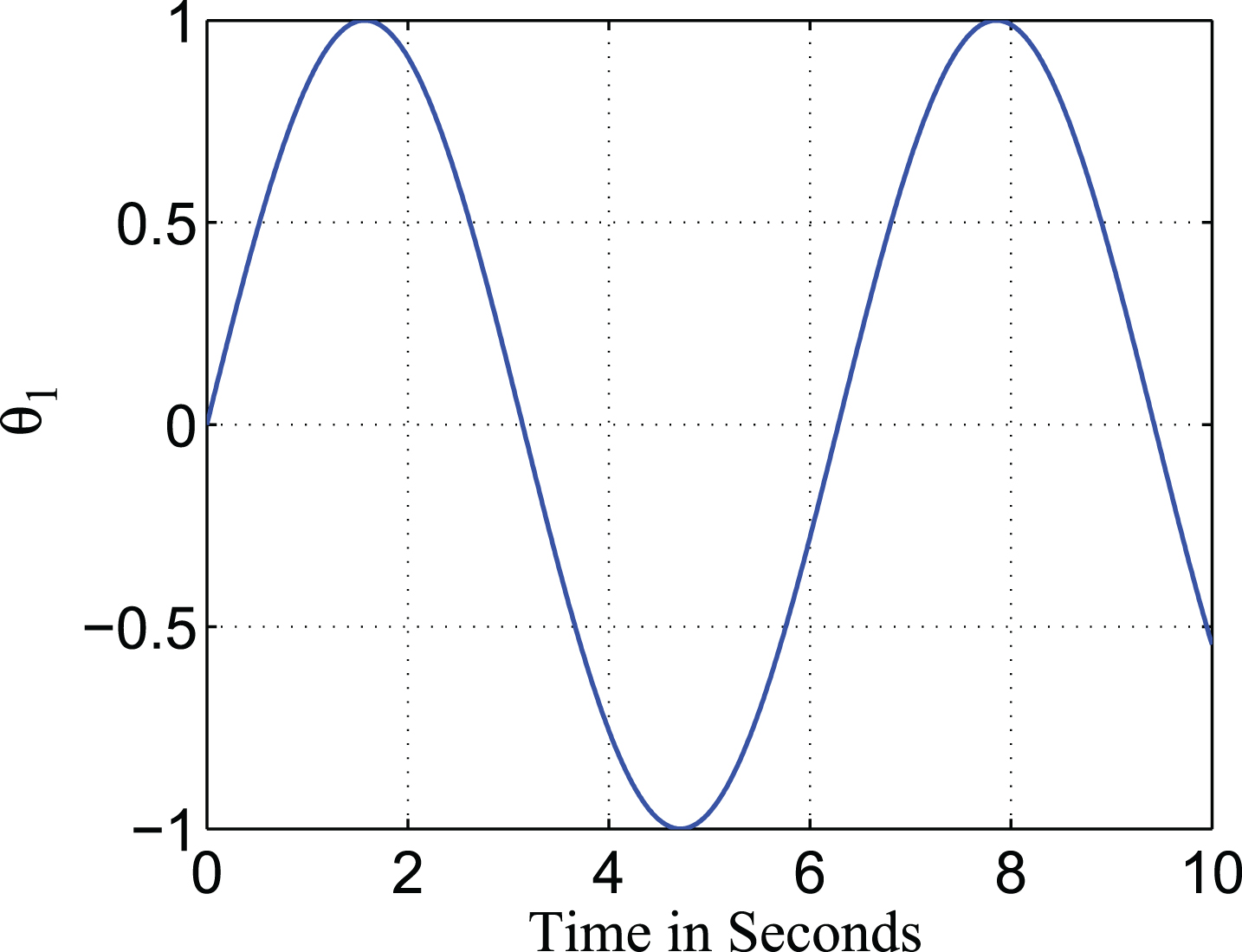
where x = [x₁ x₂] ^T is the system state, θ = θ₁ = sin(x₁) (seeing Fig. 1), and the membership functions (seeing Fig. 2) are selected as $\begin{matrix} h_{1} (x_{1}) = \frac{1 + sin (x_{1})}{2}, h_{2} (x_{1}) = \frac{1 - sin (x_{1})}{2} . \end{matrix}$

Fig.1

Parameter θ₁.

Fig.2

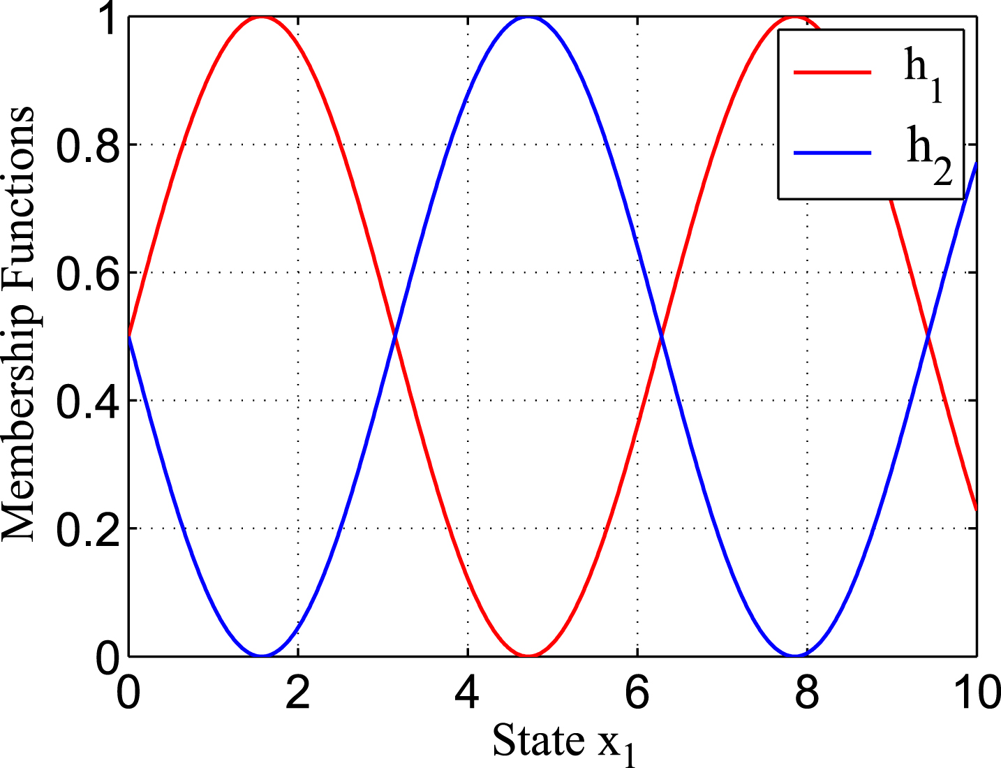
Membership functions.

The system parameter matrices for the two local linear varying systems are listed as below. $\begin{matrix} A_{10} & = & [\begin{matrix} 8 & - 1 \\ 6 & - 1 \end{matrix}], A_{11} = [\begin{matrix} a & - 2 \\ 2 & 1 \end{matrix}], \\ B_{10} & = & [\begin{matrix} 2 \\ 4 \end{matrix}], B_{11} = [\begin{matrix} - 2 \\ 3 \end{matrix}], \\ A_{20} & = & [\begin{matrix} - 5 & b \\ 2 & - 3 \end{matrix}], A_{21} = [\begin{matrix} - 3 & 5 \\ 6 & 1 \end{matrix}], \\ B_{20} & = & [\begin{matrix} - 2 \\ 10 \end{matrix}], B_{21} = [\begin{matrix} - 9 \\ 6 \end{matrix}], \end{matrix}$

where the parameters a, b ∈ [0, 10] are adjustable to compare the Theorems 3.1, 3.2 and 3.3. The system (27) is unstable for any a, b ∈ [0, 10]. From Fig. 3, the stabilization region of Theorems 3.1 and 3.2 is the small. Theorem 3.3 has a bigger stabilization region than Theorems 3.1 and 3.2. It verifies that the result of Theorem 3.3 is easily find a full states feedback fuzzy gain schedule controller. In Figs. 4 and 5, the controller in Theorem 3.3 is also effective. Therefore, the simulation verifies our the efficiency of our results.

Fig.3

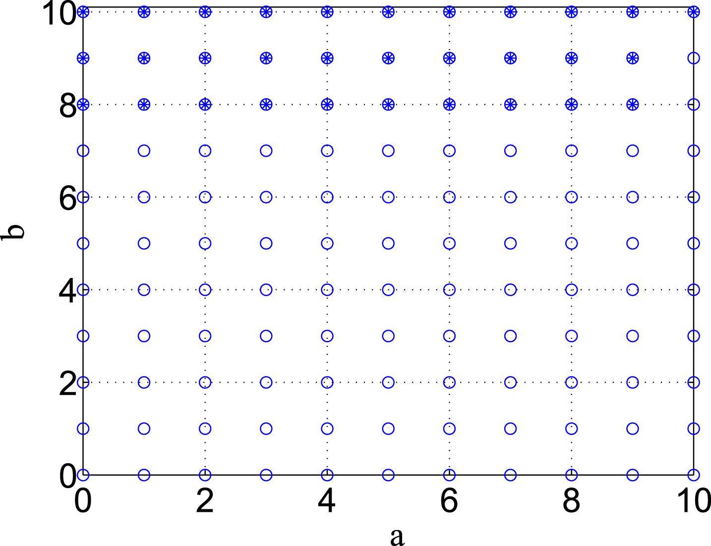
Stabilization region. Legend: {∘} → Theorem 3.3, {∗} → Theorems 3.1 or 3.2.

Fig.4

States response for a = 2, b = 5 with small initial values.

Fig.5

States response for a = 2, b = 5 with big initial values.

5 Conclusion

In the article, for the novel nonlinear time-varying model termed as the fuzzy parameter varying system, the stability analysis and controller design of the closed-loop FPV system are derived. Moreover, full-state feedback fuzzy gain-scheduling controller and self-adaption about the varying parameter θ controllers are synthesized to stabilize the closed-loop FPV system. Numerical examples are provided to demonstrate the application of our approaches to design fuzzy gain-scheduling controllers and validate the effectiveness of our results.

References

Ahammed

A.K.I.

, Profoundly robust controlling strategy for uncertain nonlinear mimo system using T-S fuzzysystem, International Journal of Fuzzy Systems 19(4) (2017), 1104–1117.

Nguyen

A.-T.

, Raymundo

and Thierry-Marie

et al. G.

, Improved lmi conditions for local quadratic stabilization ofconstrained takagi-sugeno fuzzy systems, International Journal of Fuzzy Systems 19(1) (2017), 225–237.

Apkarian

and Gahinet

, A convex characterization of gain-scheduled H-infinity controllers, IEEETransactions on Automatic Control 40(5) (1995), 853–864.

Faycal

, Kevin

and Noureddine

et al. M.

, Relaxed controller design conditions for takagi-sugeno systems withstate time-varying delays, International Journal of Fuzzy Systems 19(5) (2017), 1406–1416.

Stephen

P.B.

, Lieven

Convex Optimization, Cambridge University Press, Cambridge, UK; New York, 2004.

Haj

B.I.

, Mohamed

and Driss

, Fault-tolerant control for T-S fuzzy descriptor systems with sensor faults: Anlmi approach, International Journal of Fuzzy Systems 19(2) (2017), 516–527.

Ying-Jen

, Hiroshi

and Kazuo

et al. T.

, Relaxed stabilization criterion for T-S fuzzy systems by minimum-typepiecewise-lyapunov-function-based switching fuzzy controller, IEEE Transactions on Fuzzy Systems 20(6) (2012), 1166–1173.

Jiuxiang

, Guang-Hong

and Huaguang

, Stability analysis of T-S fuzzy control systems by using set theory, IEEE Transactions on Fuzzy Systems 23(4) (2015), 827–841.

Shuchen

, Xianlin

and Xiaojun

et al. B.

, Type-2 fuzzy logic control for underactuated truss-like roboticfinger with comparison of a type-1 case, Journal of Intelligent & Fuzzy Systems 33(4) (2017), 2047–2057.

10.

Galvan-Guerra

, Fridman

and Davila

, High-order sliding-mode observer for linear time-varying systems withunknown inputs, International Journal of Robust and Nonlinear Control 27(14) (2017), 2338–2356.

11.

Guelton

, Bouarar

and Manamanni

, Robust dynamic output feedback fuzzy lyapunov stabilization oftakagi-sugeno systems-a descriptor redundancy approach, Fuzzy Sets and Systems 160(19) (2009), 2796–2811.

12.

and Woo

P.Y.

, Fuzzy supervisory sliding-mode and neural-network control for robotic manipulators, IEEETransactions on Industrial Electronics 53(3) (2006), 929–940.

13.

Jetto

, Orsini

and Romagnoli

, Modeling and quadratic stabilization of a class of linear uncertaintime-varying systems, International Journal of Robust and Nonlinear Control 27(10) (2017), 1810–1825.

14.

Kim

S.H.

, Relaxation technique for a T-S fuzzy control design based on a continuous-time fuzzyweighting-dependent lyapunov function, IEEE Transactions on Fuzzy Systems 21(4) (2013), 761–766.

15.

Kwon

O.M.

, Park

M.J.

and Lee

et al. S.M.

, Augmented lyapunov-krasovskii functional approaches to robust stabilitycriteria for uncertain takagi-sugeno fuzzy systems with time-varying delays, Fuzzy Sets and Systems 201 (2012), 1–19.

16.

Lei

F.R.

, Xu

X.F.

and Li

et al. T.

, Attitude tracking control for mars entry vehicle via T-S model withtime-varying input delay, Nonlinear Dynamics 85(3) (2016), 1749–1764.

17.

H.Y.

, Jing

X.J.

and Lam

et al. H.K.

, Fuzzy sampled-data control for uncertain vehicle suspension systems, IEEE Transactions on Cybernetics 44(7) (2014), 1111–1126.

18.

H.B.

, Wu

L.G.

and Li

et al. J.T.

, Stabilization and separation principle of networked control systems using theT-S fuzzy model approach, IEEE Transactions on Fuzzy Systems 23(5) (2015), 1832–1843.

19.

Jinliang

and Dong

, Asymptotic and robust stability of T-S fuzzy genetic regulatory networks withtime-varying delays, International Journal of Robust and Nonlinear Control 22(8) (2012), 827–840.

20.

Liu

, A gain-scheduling control approach for takagi-sugeno fuzzy systems based on linear parameter-varyingcontrol theory, Journal of Dynamic Systems Measurement and Control-Transactions of the Asme 138(1) (2016).

21.

Liu

, Gain-scheduling control of T-S fuzzy systems with actuator saturation, Journal of Intelligent &Fuzzy Systems 32(3) (2017), 2579–2589.

22.

Liu

, Dynamic output feedback control for continuous-time T-S fuzzy systems using fuzzy lyapunov functions, IEEE Transactions on Fuzzy Systems 25(5) (2017), 1155–1167.

23.

Park

M.J.

and Kwon

O.M.

, Stability and stabilization of discrete-time T-S fuzzy systems with time-varying delayvia cauchy-schwartz-based summation inequality, IEEE Transactions on Fuzzy Systems 25(1) (2017), 128–140.

24.

Peng

and Fei

M.R.

, An improved result on the stability of uncertain T-S fuzzy systems with intervaltime-varying delay, Fuzzy Sets and Systems 212 (2013), 97–109.

25.

Rotondo

, Puig

and Nejjari

et al. F.

, Automated generation and comon of takagi-sugeno and polytopicquasi-LPV models, Fuzzy Sets and Systems 277 (2015), 44–64.

26.

Arash

, Gain-scheduled filtering for linear parameter-varying systems using inexact scheduling parameters withbounded variation rates, International Journal of Robust and Nonlinear Control 26(13) (2016), 2864–2879.

27.

Selvaraj

, Sakthivel

and Kwon

et al. O.M.

, Disturbance rejection of interval type-2 fuzzy systems based onequivalence-input-disturbance approach, Journal of Dynamic Systems Measurement and Control-Transactions ofthe Asme 139(10) (2017).

28.

Sheng

S.Y.

and Zhang

X.M.

, H-infinity filtering for T-S fuzzy complex networks subject to sensor saturation viadelayed information, Iet Control Theory and Applications 11(14) (2017), 2370–2382.

29.

Tanaka

, Ohtake

and Wang

H.O.

, A descriptor system approach to fuzzy control system design via fuzzylyapunov functions, IEEE Transactions on Fuzzy Systems 15(3) (2007), 333–341.

30.

Xiao

H.Q.

, He

and Wu

et al. M.

, New results on H-infinity tracking control based on the T-S fuzzy model forsampled-data networked control system, IEEE Transactions on Fuzzy Systems 23(6) (2015), 2439–2448.

31.

Yang

W.L.

, Feng

and Zhang

T.J.

, Robust model predictive control for discrete-time takagi-sugeno fuzzy systemswith structured uncertainties and persistent disturbances, IEEE Transactions on Fuzzy Systems 22(5) (2014), 1213–1228.

32.

Yin

, Shi

and Yang

H.Y.

, Adaptive fuzzy control of strict-feedback nonlinear time-delay systems withunmodeled dynamics, IEEE Transactions on Cybernetics 46(8) (2016), 1926–1938.

33.

Ying

, Ding

Y.S.

and Li

et al. S.K.

, Comon of necessary conditions for typical takagi-sugeno and mamdanifuzzy systems as universal approximators, IEEE Transactions on Systems Man and Cybernetics Part a-Systemsand Humans 29(5) (1999), 508–514.

34.

and Li

X.O.

, Fuzzy identification using fuzzy neural networks with stable learning algorithms, IEEETransactions on Fuzzy Systems 12(3) (2004), 411–420.

35.

, Moreno-Armendariz

M.A.

and Rodriguez

F.O.

, System identification using hierarchical fuzzy neural networkswith stable learning algorithm, Journal of Intelligent & Fuzzy Systems 18(2) (2007), 171–183.

36.

and Li

X.O.

, On-line fuzzy modeling via clustering and support vector machines, Information Sciences 178(22) (2008), 4264–4279.

37.

Yuan

C.Z.

, Liu

and Wu

et al. F.

, Hybrid switched gain-scheduling control for missile autopilot design, Journal of Guidance Control and Dynamics 39(10) (2016), 2352–2363.