Data mining model for multimedia financial time series using information entropy

Abstract

At present, KDD research covers many aspects, and has achieved good results in the discovery of time series rules, association rules, classification rules and clustering rules. KDD has also been widely used in practical work such as OLAP and DW. Also, with the rapid development of network technology, KDD research based on WEB has been paid more and more attention. The main research content of this paper is to analyze and mine the time series data, obtain the inherent regularity, and use it in the application of financial time series transactions. In the financial field, there is a lot of data. Because of the huge amount of data, it is difficult for traditional processing methods to find the knowledge contained in it. New knowledge and new technology are urgently needed to solve this problem. The application of KDD technology in the financial field mainly focuses on customer relationship analysis and management, and the mining of transaction data is rare. The actual work requires a tool to analyze the transaction data and find its inherent regularity, to judge the nature and development trend of the transaction. Therefore, this paper studies the application of KDD in financial time series data mining, explores an appropriate pattern mining method, and designs an experimental system which includes mining trading patterns, analyzing the nature of transactions and predicting the development trend of transactions, to promote the application of KDD in the financial field.

Keywords

Information entropy data mining financial time series clustering multimedia

1 Introduction

Data mining in the financial field, time-series transaction data is one of the main objects of mining [1], the main technical means used are: The data is preprocessed, its intrinsic mode is analyzed, and the data is analyzed and predicted according to the model [2]. There are two main research purposes of this topic. First, according to the results of the pattern analysis, the time series data is classified into: can be classified as mode and cannot be classified as mode [3 –5]. For those who cannot be classified as a model, that is, it is considered to be an isolated point, to complete the work of isolated point discovery [6]. The significance of finding isolated points is that they help to find abnormal transactions in financial transactions. It is very important to find abnormal transactions in financial transactions, so we can monitor illegal transactions such as money laundering to control financial risks. Because the identification of illegal transactions in the financial field involves many aspects and is a complex system engineering, we cannot simply take the analysis of financial time series data as the sole basis, and identify the isolated points as illegal transactions [7 –10]. However, this is not to say that it is meaningless to find isolated points in time-series transactions.

Cluster analysis is also a very important part of financial time series mining, which is usually used to provide advance classification results for other data mining tasks [11 –13]. In this paper, a clustering algorithm based on HDTW is proposed [14]. The idea of shared nearest neighbor similarity degree (SNN) is used to construct the similarity counting matrix between sequences, and the similarity counting matrix is used to find the cluster center sequence. A better clustering effect was obtained [15]. Then, a hierarchical clustering algorithm based on DTW is proposed. This method specially aims at the event similarity that meets the needs of users, and uses the comparison of similarity between classes and general distance between classes as the basis of judging the distance between classes, which greatly improves the clustering effect [16]. Finally, a real-time clustering algorithm based on morphological features for multi-time series data streams is proposed. Aiming at the characteristics of financial time series, we extract sub-sequence feature information by retaining important feature points in the data outline design [17]. When new data arrives, we use a dynamic sliding window design to ensure data synchronization among multiple data streams. This algorithm can cluster data streams at any time, and can track the evolution process of clustering results in real time [18 –20].

2 Data entropy-based data mining technology

2.1 Overview of information entropy

In mathematics, there is such an explanation.

If there is an isolated system, $\oint \frac{dQ}{T} \leq 0$ , where dQ denotes all the heat absorbed by the system from a heat source with temperature T, the equal sign denotes that the process is reversible.

Assuming that the isolated system changes from state A to state B, the process of transformation is abbreviated as AB, and the inverse process is BA. A to B form a reversible cycle, which is expressed by Clausius formula as follows: $\oint \frac{dQ}{T} = \int_{B}^{A} \frac{dQ}{T} + \int_{A}^{B} \frac{dQ}{T} = 0$ (1)

The formula shows that the value of $\oint \frac{dQ}{T}$ is independent of its process and only related to the state of A and B.

Here, the physicist Clausius introduced the entropy in thermodynamics to represent the function of the thermodynamic parameters of the system. Its change is described as $dS = \frac{dQ}{T}$ .

By 1872, another physicist, Boltzmann, had studied and expanded the theory of entropy from molecular motion, introducing the definition of “statistical entropy”. He first proposed the concept of micro-state (micro-state refers to a possible configuration of the number of particles in the system). Boltzmann recorded the number of micro-states corresponding to the macro-state as Ω. Then the relationship between the number of micro-states Ω and the entropy s is the famous Boltzmann relation: S = k ln Ω. Among them, k is Boltzmann constant. Therefore, Boltzmann gives a statistical meaning of entropy, that is, entropy is the logarithm of the number of micro-states Ω. The more the number of micro-states of the system, the greater the entropy value, that is to say, the size of the entropy directly reflects the complexity of the distribution of the micro-states of the system. Also, statistical entropy has another form of representation. Assume that the number of micro-states of the system is Ω. According to Boltzmann’s equal probability principle, the probability p of each micro-state is equal, which is 1/Ω, that is, p = 1/Ω, so the above formula can also be expressed as: $S = - k \sum \frac{1}{Ω} ln \frac{1}{Ω} = - k \sum p ln p$ (2)

It is because of Boltzmann statistics defines entropy, it soon became a viable concept. It is no longer just a concept and development of thermodynamics and statistical physics, but its practical application is far beyond the scope of physics. It directly or indirectly by adding several different areas of information theory, probability theory, and life sciences and social sciences. Then in 1948, Shannon, a gifted engineer and founder of modern information theory, introduced Boltzmann’s definition of entropy into information theory. The American scientist believes that if the probability of a signal in a source is pi, then the amount of information it brings is - ln pi. If there are only n kinds of signals used by this information source to represent information, then the probability of each signal appearing is equal (all p), then the information brought by each signal of this information source is: $S = - k \sum_{1}^{n} p ln p$ (3)

It can be said, Shannon discovered the essence of consistency between the information and the thermodynamics of communication sciences in entropy, so he used directly in thermodynamics, “entropy” is the word to express the information he studies, and the introduction of “information entropy”. When different signals from information sources have different occurrence probabilities, Shannon defines information entropy as: $S = - c \sum_{1}^{n} pi ln pi$ (4)

Here c is a constant, a quantity related to the unit of measure of information. For example, suppose the s unit is nat and c is 1. If the unit of S is bit, the value of c is 1/ln 2. Shannon extracted entropy from physics, applied it to communication theory and expanded the concept of entropy. Entropy at this time has nothing to do with thermodynamics and micro-molecular motion. Its expansion shows us its close relationship with probability theory. Above all, this shows us its most essential thing, that is, to give a scientific measurement of the “state” of the material system. Formula (4) is the expression of information entropy of discrete random variables. For continuous random variables, information entropy can be expressed as follows: $S = - c \int_{- \infty}^{+ \infty} f (x) ln f (x) dx$ (5)

In the formula above, f(x) is the probability density distribution function of continuous random variable x. Here is an example to understand the meaning of information entropy. Assuming that a coin is tossed, the probability of both the front and the back sides of the coin is 1/2, then according to formula (4), the value of entropy is calculated and the result is as follows: $S = - \frac{1}{2} ln (\frac{1}{2}) - \frac{1}{2} ln (\frac{1}{2}) = 0.693$ Assuming that a dice is thrown, the result is equivalent to six equal probability outcomes, and its entropy value is the sum of six $- \frac{1}{6} ln (\frac{1}{6})$ , namely ln6nat. If a continuous variable x is assumed to appear equally on the (a, b) region, then the entropy of the variable is calculated according to formula (5) to obtain S = ln(b - a) (nat).

From the above examples, we can see that information entropy is the uncertainty test of the observation results after an observation of the information source (or a sampling of the set). Mathematically, as long as we know the probability distribution (or probability density) of variables, we can calculate the corresponding entropy value. That is to say, entropy is the function of probability (density) distribution.

2.2 Dynamic time warping (DTW)

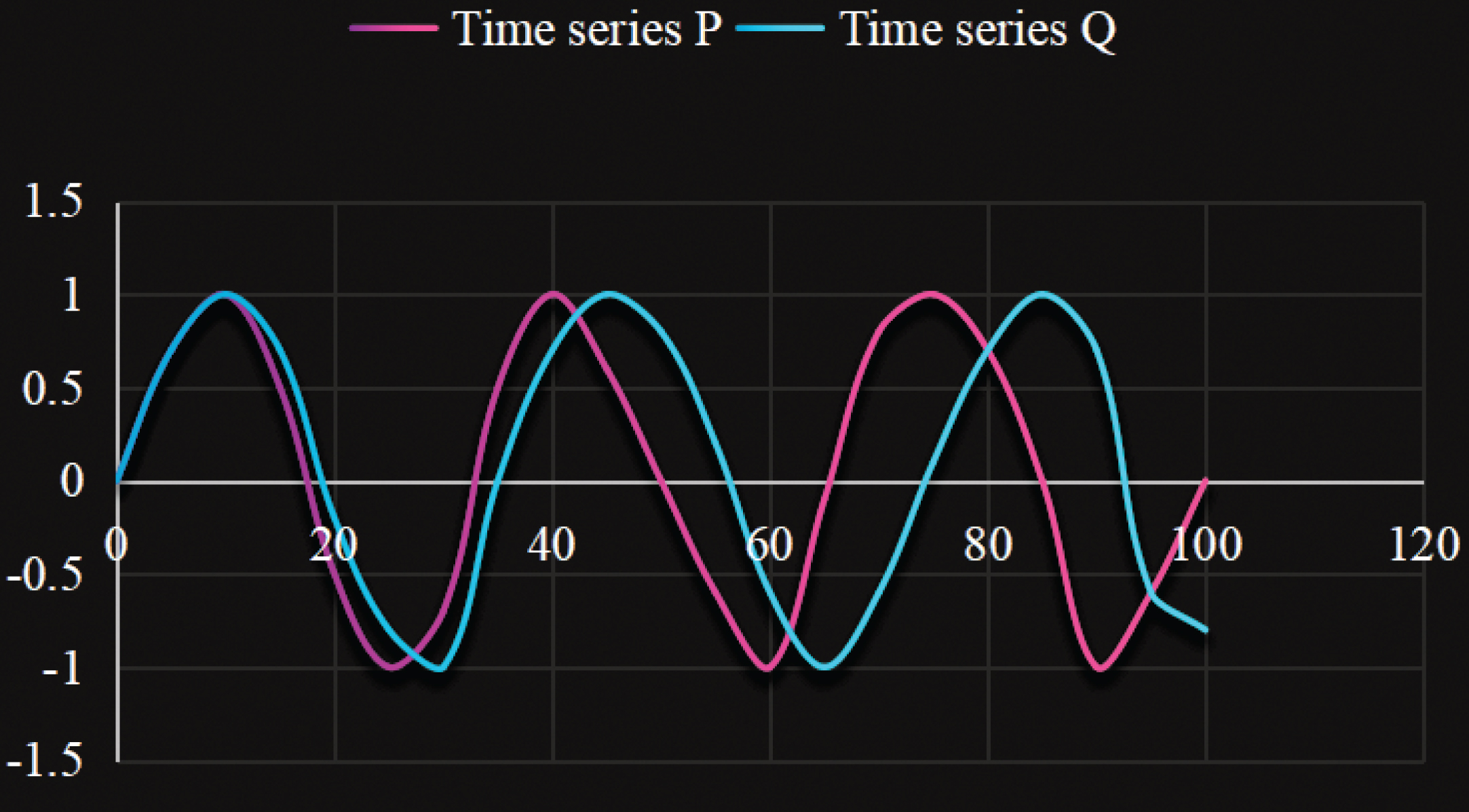
The dynamic time-bending distance between two-time series is the smallest cumulative distance among all the correspondences, and this correspondence is also the optimal correspondence.

Let two time series of lengths n and m, P = {p₁, p₂, . . . , p_n} and Q = {q₁, q₂, . . . , q_m}, to better explain how DTW corresponds to points in time series P and Q, we usually construct a matrix of n × m, called distance matrix D_base = (d_base (p_i, q_j)) _n×m. The first (i, j) element in the distance matrix is the basic distance between the point p_i in time series P and the point q_j in time series Q. The basic distance used in d_base (p_i, q_j) is: $d_{base} (x, y) = (x - y)^{2}$ (6)

At the same time, the first (i, j) element in the distance matrix also indicates that the point P_i in time series P corresponds to the point q_i in time series Q. Selecting a series of continuous elements in the distance matrix can obtain a corresponding relationship between two-time series, also known as a curved path. To obtain the dynamic time-bending distance, only one optimal bending path is found to minimize the cumulative sum of elements in the distance matrix through which it passes, as shown in Fig. 1:

2.2.1 Shortcomings of dynamic time bending

Fig.1

Distance matrix and curved path graph between two-time series.

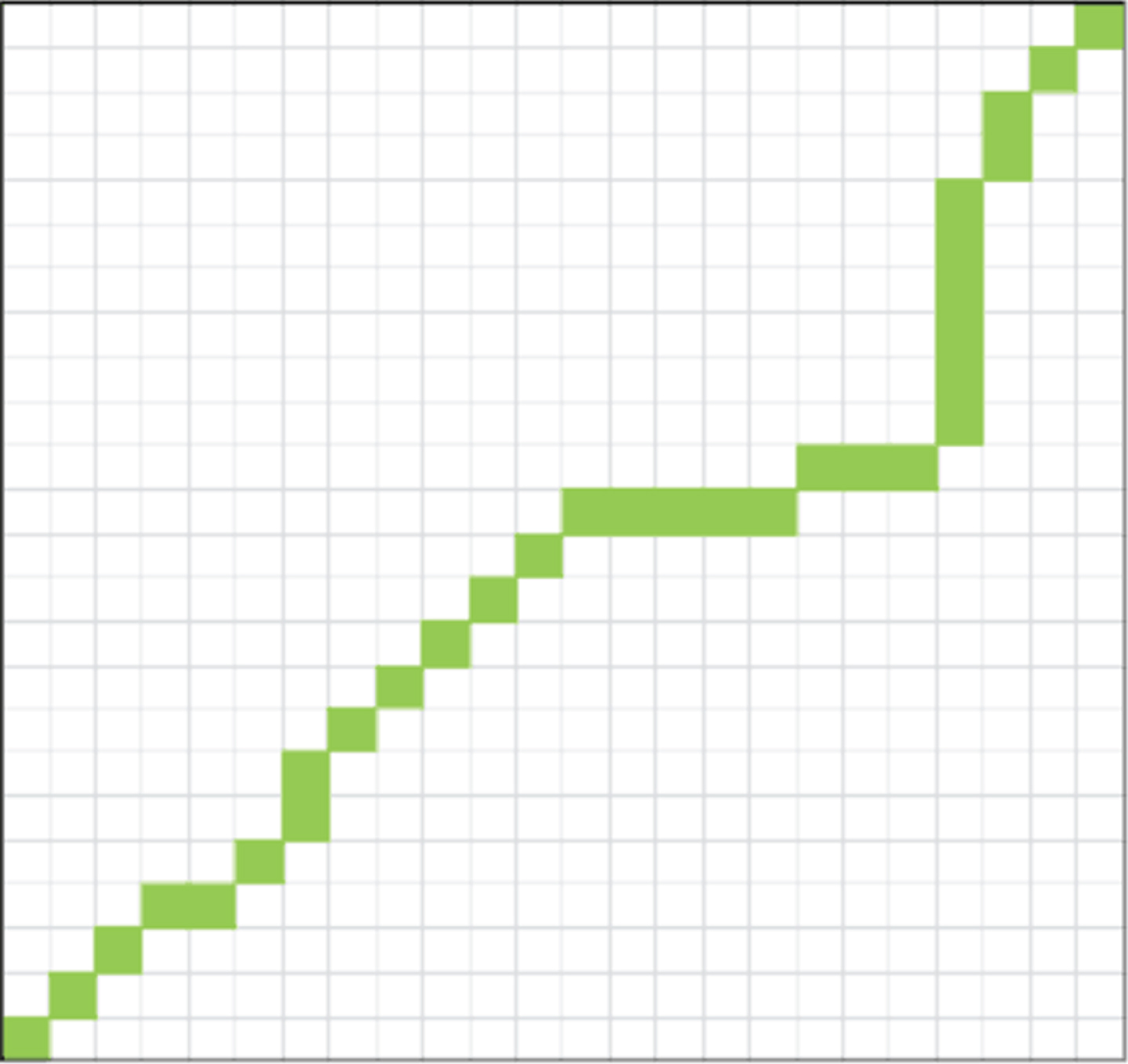
The best way to correspond between two-time series should be that the same characteristics correspond to each other, such as the peak on one time series corresponds to the peak on another time series, rather than a valley. When the original DTW solves the optimal bending path by dynamic programming, it may blindly seek the minimum cumulative distance of the optimal bending path, and correspond multiple times in one-time series to another time series, as shown in Figure 2. The data in the graph is taken from ECG200 data set in UCR Time Series Archive. It can be seen from the graph that the points of the above time series correspond to one point of the following time series. The most common case is that the 29 points of the above time series correspond to one point of the following time series. That is to say, the above time series is severely compressed, and the characteristics of the sequence fragments are ignored in the process of compression. The same time series is compressed.

Fig.2

Correspondence diagram of two-time series under DTW.

Excessive compression results in the loss of features of time series, and the original DTW is no longer accurate in describing the distance between time series. Therefore, various time series mining algorithms based on the original DTW will have inaccurate problems, such as the correct classification rate of the KNN classification algorithm based on the original DTW will decrease.

2.2.2 Hierarchical clustering

Because of these shortcomings, this paper chooses the hierarchical clustering method. Hierarchical clustering is also a very common clustering method, in which the “bottom-up” hierarchical clustering method is used more frequently. The basic steps are:

Calculate the distance between two of n data points;

Each data point is considered as a single class, that is, n C₁, C₂, . . . , C_n are constructed;

Find two nearest C_i, C_j classes, merge them into one class and turn them into n-1 classes;

Calculate the spacing between the new class and other classes in this layer. If the termination condition (number of clusters or minimum spacing) is satisfied, stop, otherwise turn (2).

It can be seen that the hierarchical distance method first considers the nearest neighbor, so the closer the two points are, the more likely they are in a class. The key of hierarchical clustering is how to determine the distance between classes. There are mainly the following methods:

Single connection method, also known as the shortest distance method, that is, the distance between two classes is defined as the smallest of the elements in the two classes;

Full connection method, also known as the longest distance method, that is, the distance between two classes is defined as the maximum between the two classes of elements;

Average distance method, that is, the average distance between two elements in two classes is taken as the distance between classes;

Central method, that is, the distance between the centers of gravity between two classes as the distance between classes;

Ward method, whose thought is similar to the idea of variance analysis. The purpose is to make the square of the dispersion within the class as small as possible, and the square of the dispersion between the class and the class as large as possible. Its calculation formula is: $D (C_{i}, C_{j}) = σ_{i + j}^{2} - σ_{i}^{2} - σ_{j}^{2}$ (7)

Among them, $σ_{i + j}^{2}$ is the sum of squared deviations after the combination of class C_i, C_j, and $σ_{i}^{2}$ , $σ_{j}^{2}$ is the sum of squared deviations of each class C_i, C_j.

3 System-controlled experimental scheme of data set

(1) Data set

Data set 1: SCCTS (Systhetic Control Chart Time Series) is a network open test set, specially used for algorithm testing of time series clustering. SCCTS has 600 test data, which belong to six different categories. Ten sets of data were extracted from the data set (SCCTS). Each group of data contains 60-time series, which belongs to 6 different categories and 10 in each category.

Data Set 2 : 10 groups of data in data set 1 are processed unequally. Without affecting the clustering results, the length of 60-time series in each group of data is not the same. The experiments in this chapter are based on the above two data sets.

(2) Experimental scheme

Experiments 1: Dynamic Time Warping (DTW) and Hierarchical Dynamic Time Warping (HDTW) are used to cluster data set 1, and the clustering accuracy and efficiency of the two methods are compared.

Experiment 2: DTW and HDTW were used to cluster data set 2, and the clustering accuracy and efficiency of the two methods were compared.

(3) Application of Multimedia Technology in Time Series Data Mining of Financial Time Series

Figure 3 shows the financial time series diagram. Figure 4 shows the characteristic classification of financial time series. Through the media technology, we can intuitively convey the key aspects and characteristics, to achieve in-depth insight into the rather sparse and complex data sets.

Fig.3

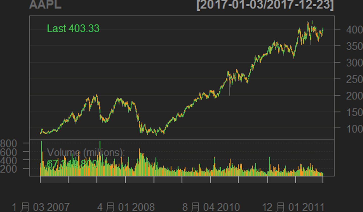
Financial Time Series Diagram with Multimedia Technology.

Fig.4

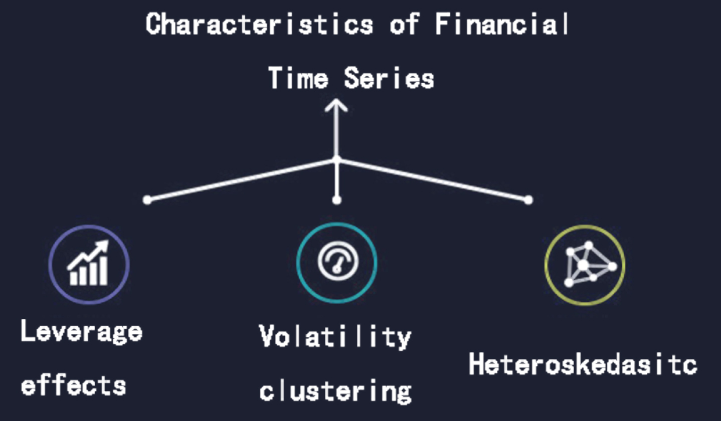
Characteristic Classification of Multimedia Financial Time Series.

4 Analysis of clustering conclusion based on information entropy

(1) Analysis of the results of Experiment 1

Experiment 1 compares the advantages and disadvantages of the DTW and the HDTW through the equal time series data set 1. In HDTW method, the number of layers for similarity measurement can be selected by setting the parameter k. Figure 5 shows the variation of the average clustering accuracy of the ten sets of data in the HDTW algorithm as the number of selected layers changes. The horizontal axis represents the number of layers k selected, ranging from 1–20, and the vertical axis represents the average clustering accuracy of ten sets of data. It can be seen from the figure that the clustering precision obtained by the HDTW method is between 0.78 and 0.9, and the number of layers k has no obvious linear relationship with the average clustering accuracy. However, a higher average clustering accuracy can be obtained when the number of layers is in the range of 15–19.

Fig.5

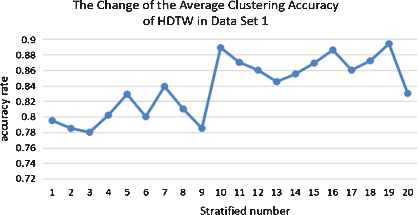
The average clustering accuracy change chart of HDTW algorithm in data set 1.

Figure 6 shows the comparison of clustering accuracy between DTW algorithm and HDTW algorithm on each group of data. The horizontal axis represents 10 groups of data in data set 1, and the vertical axis represents the clustering accuracy of each group of data using two methods respectively. It can be seen from the figure that the clustering precision obtained by the DTW method is between 0.65 and 0.9, and the clustering precision obtained by the HDTW algorithm is between 0.75 and 0.9. And in addition to the 10th set of data, the clustering accuracy obtained by the HDTW algorithm is always higher than that of the DTW algorithm. Figure 7 shows a comparison of the total average clustering accuracy of 10 sets of data. It can be seen from the figure that the HDTW algorithm results are far superior to the DTW algorithm. The clustering accuracy obtained by the similarity measure by the HDTW algorithm is nearly 10% higher than the DTW algorithm.

Fig.6

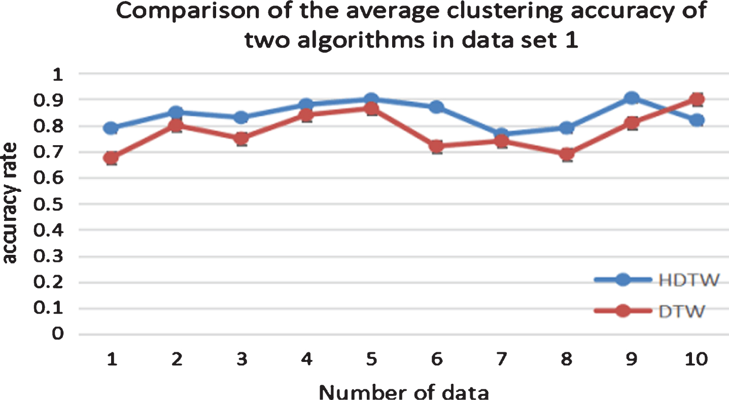
Comparison of the average clustering accuracy of each group of the two algorithms in data set 1.

Fig.7

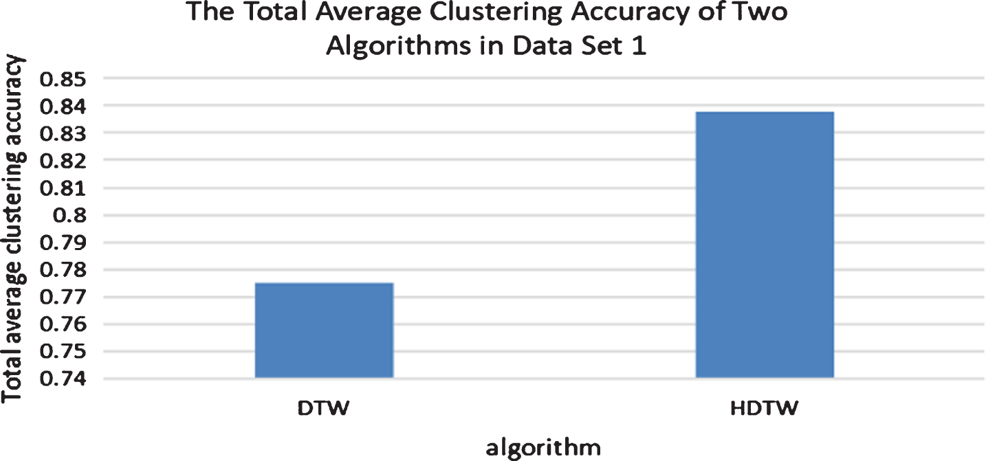
Comparison of the total average clustering accuracy of the two algorithms in data set 1.

(2) Analysis of the results of Experiment 2

Experiment 2 compares the advantages and disadvantages of DTW method and HDTW method through unequal time series data set 2.

From Fig. 8, we can see that the clustering accuracy obtained by HDTW method is between 0.8 and 0.92, and the number of layers k selected has no obvious linear relationship with the final average clustering accuracy. However, when the number of layers is between 10 and 13, higher clustering accuracy can be obtained.

Fig.8

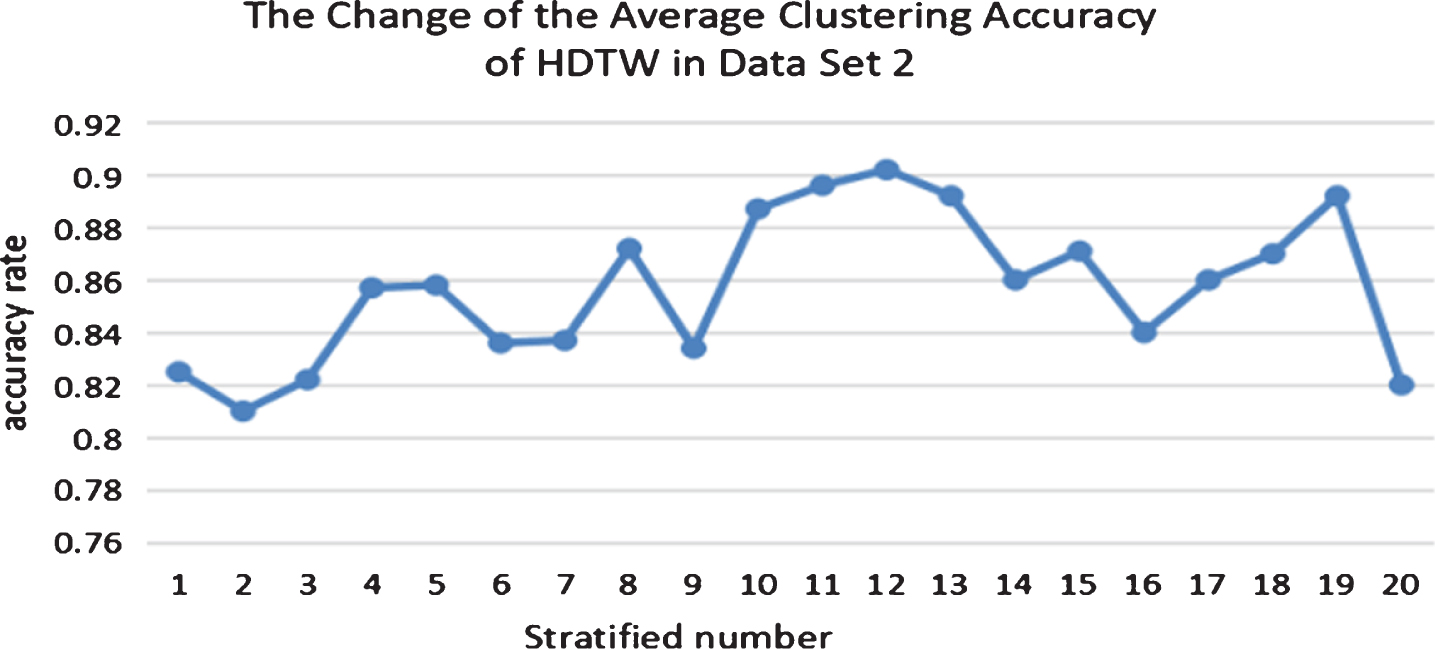
Average clustering accuracy change of HDTW algorithm in data set 2.

Comparing Figs. 6 and 9, we can find that HDTW algorithm can achieve a better clustering effect on unequal data set 2 than on data set 1.

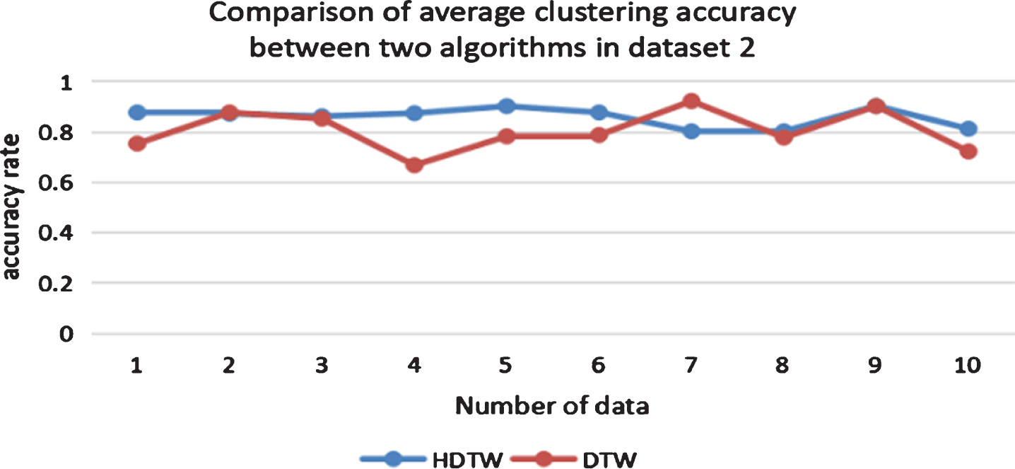
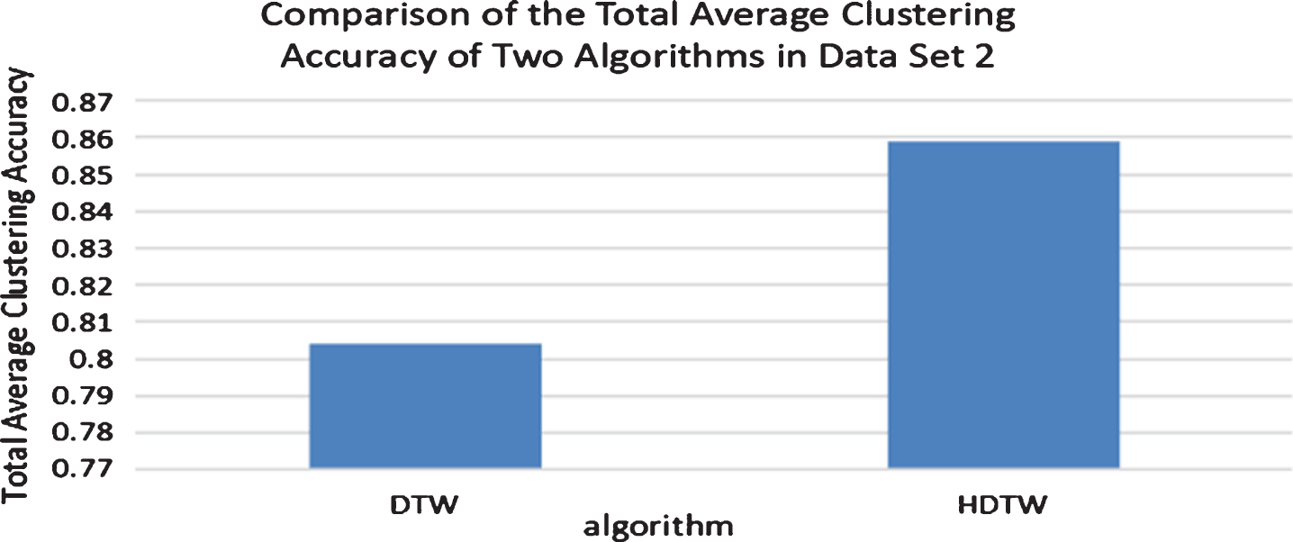
As can be seen from Fig. 9, the clustering accuracy of DTW method is between 0.65 and 0.95, and the clustering accuracy of different data groups fluctuates greatly. The clustering accuracy of HDTW algorithm is between 0.8 and 0.9, and the clustering accuracy of different data groups fluctuates slightly. Except for the seventh group of data, the clustering accuracy of HDTW algorithm is always higher than that of DTW algorithm. Figure 10 shows the comparison of the total average clustering accuracy of 10 groups of data. It can be seen from the figure that the result of HDTW algorithm is better than that of DTW algorithm.

Fig.9

Comparison of average clustering accuracy between two algorithms in data set 2.

Fig.10

Comparison of the total average clustering accuracy of the two algorithms in data set 2.

5 Conclusions

(1) Compared with the traditional algorithm, HDTW algorithm has a great advantage in clustering data sets. HDTW breaks the global invariance of DTW parameters and realizes parameter adaptation. This provides a direction for good clustering of data sets with different densities.

(2) Compared with the traditional single method, such as SVR and SOFM, financial time series prediction. The improved algorithm of DTW proposed in this paper, HDTW, can establish a regression prediction model by finding a large number of similar classes, and improve the accuracy of the prediction of stock price and financial index.

(3) Experiments show that HDTW algorithm has certain robustness to unsteady and non-linear data, can establish a reliable model with obvious effect, and can predict the next day’s stock growth better.

References

Silva

J.A.

, Faria

E.R.

, Barros

R.C.

, et al., Data stream clustering: A survey, ACM Computing Surveys (CSUR) 46(1) (2013), 1–31.

Brouwer

R.K.

A method of relational fuzzy clustering based on producing feature vectors using FastMap, Information Sciences 179(20) (2009), 3561–3582.

Hsu

S.H.

, Hsieh

J.J.P.A.

, Chih

T.C.

, et al., A two-stage architecture for stock price forecasting by integrating self-organizing map and support vector regression, Expert Systems with Applications 36(4) (2009), 7947–7951.

Mohamed

A comparative study on the Internet of Things (IoT): Frameworks, Tools, Applications and Future Directions, Journal of Intelligent Systems and Internet of Things 1(1) (2020), 13–39.

Mohamed

The Relation of Artificial Intelligence with Internet Of Things: A survey, Journal of Cybersecurity and Information Management 1(1) (2020), 30–24.

Wang

, Chen

, Lu

A very fast algorithm for detecting community structures in complex networks, Physica A: Statistical Mechanics and its applications 384(2) (2007), 667–674.

Fan

, Li

, Zhang

, et al., The effect of weight on community structure of networks, Physica A: Statistical Mechanics and its applications 378(2) (2007), 583–590.

Medus

, Acuña

, Dorso

C.O.

Detection of community structures in networks via global optimization, Physica A: Statistical Mechanics and its applications 358(2-4) (2005), 593–604.

, Huberman

B.A.

Finding communities in linear time: a physics approach, The European Physical Journal B 38(2) (2004), 331–338.

10.

Lusseau

, Schneider

, Boisseau

O.J.

, et al., The bottlenose dolphin community of Doubtful Sound features a large proportion of long-lasting associations, Behavioral Ecology and Sociobiology 54(4) (2003), 396–405.

11.

Keogh

, Chakrabarti

, Pazzani

, et al., Locally adaptive dimensionality reduction for indexing large time series databases[C], Proceedings of the 2001 ACM SIGMOD international conference on Management of data (2001), 151–162.

12.

Alhabib

, Salama

A.A.

Using Moving Averages To Pave The Neutrosophic Time Series, International Journal of Neutrosophic Science 3(1) (2020), 14–20.

13.

Zaki

M.J.

SPADE: An efficient algorithm for mining frequent sequences, Machine learning 42(1-2) (2001), 31–60.

14.

Wang

Discovering patterns from large and dynamic sequential data, Journal of Intelligent Information Systems 9(1) (1997), 33–56.

15.

Faloutsos

, Ranganathan

, Manolopoulos

Fast subsequence matching in time-series databases, Acm Sigmod Record 23(2) (1994), 419–429.

16.

Chen

Y.L.

, Weng

C.H.

Mining association rules from imprecise ordinal data, Fuzzy sets and systems 159(4) (2008), 460–474.

17.

Medus

, Acuña

, Dorso

C.O.

Detection of community structures in networks via global optimization, Physica A: Statistical Mechanics and its applications 358(2-4) (2005), 593–604.

18.

Yang

, Cheung

, Liu

Community mining from signed social networks, IEEE Transactions on Knowledge and Data Engineering 19(10) (2007), 1333–1348.

19.

Fan

, Li

, Zhang

, et al., The effect of weight on community structure of networks, Physica A: Statistical Mechanics and its applications 378(2) (2007), 583–590.

20.

Estrada

, Hatano

Communicability graph and community structures in complex networks, Applied Mathematics and Computation {214(2) (2009), 500–511.