Circular intuitionistic fuzzy sets

1 Introduction

The Intuitionistic Fuzzy Sets (IFSs) were introduced in 1983 (see [1–3]) as extensions of fuzzy sets of L. Zadeh [9] and in next years have become object of a lot of extensions and modifications. Some of them – only “IFS-extensions” claiming to be.

One of the real IFS-extension is the object Interval-Valued IFS (IVIFS; see [3, 4]).

Now, the IFSs have a lot of geometrical interpretations. The most important one is given on Fig. 1. As it is seen from it, the elements of a fixed universe are interpreted as points on the Intuitionistic Fuzzy Interpretation Triangle (IFIT). Each element x that is evaluated with degrees of membership μ _A  (x) and of non-membership ν _A  (x) to a fixed subset A of the universe, is represented as a point with coordinates 〈μ _A  (x) , ν _A  (x) 〉, where μ _A  (x) , ν _A  (x) , μ _A  (x) + ν _A  (x) ∈ [0, 1].

In the case of IVIFS, the element x is evaluated by pair of intervals 〈M _A  (x) , N _A  (x) 〉, where M _A  (x) , N _A  (x) ⊆ [0, 1] and sup M _A  (x) + sup N _A  (x) ≤1 (see Fig. 2).

In the present paper, a real extension of the IFSs is introduced. Its elements are represented by circles in the IFIT.

2 Definition and geometrical interpretation of a Circular-IFS

Let us have a fixed universe E and its subset A. The set A r * = { 〈 x , μ A ( x ) , ν A ( x ) ; r 〉 | x ∈ E } , where 0 ≤ μ _A  (x) + ν _A  (x) ≤1 and r ∈ [0, 1] is a radius of the circle around each element x ∈ E, is called Circular-IFS (C-IFS) and functions μ _A  : Eri [0, 1] and ν _A  : Eri [0, 1] represent the degree of membership (validity, etc.) and non-membership (non-validity, etc.) of element x ∈ E to a fixed set A ⊆ E. Now, we can define also function π _A  : Eri [0, 1] by means of π _A  (x) =1 - μ _A  (x) - ν _A  (x) and it corresponds to degree of indeterminacy (uncertainty, etc.).

OPEN IN VIEWER

Fig.1

Geometrical interpretation of an element of an IFS.

OPEN IN VIEWER

Fig.2

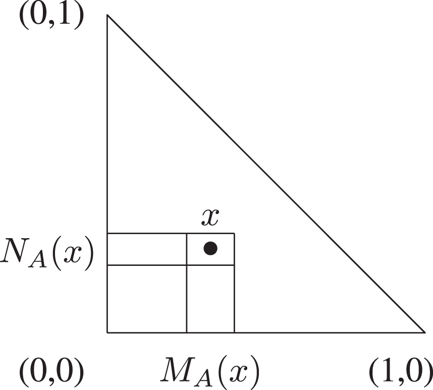
Geometrical interpretation of an element of an IVIFS.

For brevity, we shall write below A _r instead of A r * , whenever this is possible.

In contrast with the standard IFSs, where each element is represented by a point in the intuitionistic fuzzy interpretation triangle, here, each element is represented by a circle with center 〈μ _A  (x) , ν _A  (x) 〉 and radius r.

Now, the basic (second) geometrical interprepation of the C-IFS has the form from Fig. 3. OPEN IN VIEWER

We can see easily that there are five possible forms of the circles, as it is shown on Fig. 3.

Let L^* = {〈a, b〉|a, b ∈ [0, 1]   &  a + b ≤ 1} .

Therefore, A _r can be rewritten in the form A r * = { 〈 x , O r ( μ A ( x ) , ν A ( x ) ) 〉 | x ∈ E } ,

where O r ( μ A ( x ) , ν A ( x ) ) = { 〈 a , b 〉 | a , b ∈ [ 0 , 1 ] & ( μ A ( x ) - a ) 2 + ( ν A ( x ) - b ) 2 ≤ r } ∩ L * = { 〈 a , b 〉 | a , b ∈ [ 0 , 1 ] & ( μ A ( x ) - a ) 2 + ( ν A ( x ) - b ) 2 ≤ r & a + b ≤ 1 } .

The new type of sets is an extension of the standard IFS, because each standard IFS has the form A = A 0 = { 〈 x , μ A ( x ) , ν A ( x ) ; 0 〉 | x ∈ E } , but the C-IFS with r > 0 cannot be represented by a standard IFS.

Now, the relations between two C-IFSs A _r and B _s are the following: A r ⊂ v B s iff ( ∀ x ∈ E ) ( ( r = s ) & ( ( μ A ( x ) < μ B ( x ) & ν A ( x ) ≥ ν B ( x ) ) ∨ ( μ A ( x ) ≤ μ B ( x ) & ν A ( x ) > ν B ( x ) ) ∨ ( μ A ( x ) < μ B ( x ) & ν A ( x ) > ν B ( x ) ) ) ) ; A r ⊂ ρ B s iff ( ∀ x ∈ E ) ( ( r < s ) & μ A ( x ) = μ B ( x ) & ν A ( x ) = ν B ( x ) ) ; A r ⊂ B s iff ( ∀ x ∈ E ) ( ( r < s ) & ( ( μ A ( x ) < μ B ( x ) & ν A ( x ) ≥ ν B ( x ) ) ∨ ( μ A ( x ) ≤ μ B ( x ) & ν A ( x ) > ν B ( x ) ) ∨ ( μ A ( x ) < μ B ( x ) & ν A ( x ) > ν B ( x ) ) ) ) ; A r ⊃ v B s iff B s ⊂ v A r ; A r ⊃ ρ B s iff B s ⊂ ρ A r ; A r ⊃ B s iff B s ⊂ A r ; A r ⊆ v B s iff ( ∀ x ∈ E ) ( r = s & μ A ( x ) ≤ μ B ( x ) & ν A ( x ) ≥ ν B ( x ) ) ; A r ⊆ ρ B s iff ( ∀ x ∈ E ) ( r ≤ s & μ A ( x ) = μ B ( x ) & ν A ( x ) = ν B ( x ) ) ; A r ⊆ B s iff ( ∀ x ∈ E ) ( r ≤ s & μ A ( x ) ≤ μ B ( x ) & ν A ( x ) ≥ ν B ( x ) ) ; A r ⊇ v B s iff B ⊆ v A r ; A r ⊇ ρ B s iff B ⊆ ρ A r ; A r ⊇ B s iff B ⊆ A r ; A r = v B s iff ( ∀ x ∈ E ) ( μ A r ( x ) = μ B ( x ) & ν A r ( x ) = ν B ( x ) ) ; A r = ρ B s iff r = s ; A r = B s iff ( ∀ x ∈ E ) ( r = s & μ A r ( x ) = μ B ( x ) & ν A r ( x ) = ν B ( x ) ) .

The operations over C-IFSs are similar, but more complex than these over standard IFSs. They are the following:

¬ A r = { 〈 x , ν A ( x ) , μ A ( x ) ; r 〉 | x ∈ E } ; A r ∩ min B s = { 〈 x , min ( μ A ( x ) , μ B ( x ) ) , max ( ν A ( x ) , ν B ( x ) ) ; min ( r , s ) 〉 | x ∈ E } ; A r ∩ max B s = { 〈 x , min ( μ A ( x ) , μ B ( x ) ) , max ( ν A ( x ) , ν B ( x ) ) ; max ( r , s ) 〉 | x ∈ E } ; A r ∪ min B s = { 〈 x , max ( μ A ( x ) , μ B ( x ) ) , min ( ν A ( x ) , ν B ( x ) ) ; min ( r , s ) 〉 | x ∈ E } ;

A r ∪ max B s = { 〈 x , max ( μ A ( x ) , μ B ( x ) ) , min ( ν A ( x ) , ν B ( x ) ) ; max ( r , s ) 〉 | x ∈ E } ; A r + min B r = { 〈 x , μ A ( x ) + μ B ( x ) - μ A ( x ) . μ B ( x ) , ν A ( x ) . ν B ( x ) ; min ( r , s ) 〉 | x ∈ E } ; A r + max B r = { 〈 x , μ A ( x ) + μ B ( x ) - μ A ( x ) . μ B ( x ) , ν A ( x ) . ν B ( x ) ; max ( r , s ) 〉 | x ∈ E } ; A r • min B s = { 〈 x , μ A ( x ) . μ B ( x ) , ν A ( x ) + ν B ( x ) - ν A ( x ) . ν B ( x ) ; min ( r , s ) 〉 | x ∈ E } ; A r • max B s = { 〈 x , μ A ( x ) . μ B ( x ) , ν A ( x ) + ν B ( x ) - ν A ( x ) . ν B ( x ) ; max ( r , s ) 〉 | x ∈ E } ;

A r @ min B s = { 〈 x , 〈 μ A ( x ) + μ B ( x ) ) 2 , ( ν A ( x ) + ν B ( x ) ) 2 ; min ( r , s ) 〉 | x ∈ E } ; A r @ max B s = { 〈 x , 〈 μ A ( x ) + μ B ( x ) ) 2 , ( ν A ( x ) + ν B ( x ) ) 2 ; max ( r , s ) 〉 | x ∈ E } .

We will formulate two theorems which are proved in a manner analogous to the theorems for the standard IFS, see e.g. [2, 3], hence, we omit the proofs.

Theorem 1. The following equalities are valid for any three C-IFSs A _r , B _s and C _t :

A _r ∩ _minB _s  = B _s  ∩ _minA _r  ;

Theorem 2. The following inclusions are valid:

A • _minB_⊆vA ∩ _minB_⊆vA @ B_min⊆vA ∪ _minB_⊆vA + B_min,

4 Modal operators over C-IFSs

The two simplest intuitionistic fuzzy modal operators now have the forms □ A r = { 〈 x , μ A ( x ) , 1 - μ A ( x ) ; r 〉 | x ∈ E } = { 〈 x , O r ( μ A ( x ) , 1 - μ A ( x ) ) 〉 | x ∈ E } , ♦ A r = { 〈 x , 1 - ν A ( x ) , ν A ( x ) ; r 〉 | x ∈ E } = { 〈 x , O r ( 1 - ν A ( x ) , ν A ( x ) ) 〉 | x ∈ E } .

They are analogous to the modal logic operators “necessity” and “possibility” and of their intuitionistic fuzzy analogues. More complex is the form of the extended intuitionistic fuzzy modal operators.

Let α, be ∈ [0, 1] be fixed numbers. For the IFS A, these operators are: D α ( A r ) = { 〈 x , μ A ( x ) + α . π A ( x ) , = { ν A ( x ) + ( 1 - α ) . π A ( x ) ; r 〉 | x ∈ E } , D α ( A r ) = { 〈 x , O r ( μ A ( x ) + α . π A ( x ) , = { ν A ( x ) + ( 1 - α ) . π A ( x ) ) 〉 | x ∈ E } , F α , β ( A r ) = { 〈 x , μ A ( x ) + α . π A ( x ) , = { ν A ( x ) + β . π A ( x ) ; r 〉 | x ∈ E } , = { 〈 x , O r ( μ A ( x ) + α . π A ( x ) , = { ν A ( x ) + β . π A ( x ) ) 〉 | x ∈ E } , = { where α + β ≤ 1 , G α , β ( A r ) = { 〈 x , α . μ A ( x ) , β . ν A ( x ) ; r 〉 | x ∈ E } , = { 〈 x , O r ( α . μ A ( x ) , β . ν A r ( x ) ) 〉 | x ∈ E } , H α , β ( A r ) = { 〈 x , α . μ A ( x ) , ν A ( x ) + β . π A ( x ) ; r 〉 = { | x ∈ E } , = { 〈 x , O r ( α . μ A ( x ) , ν A ( x ) + β . π A ( x ) ) 〉 = { | x ∈ E } , H α , β * ( A r ) = { 〈 x , α . μ A ( x ) , ν A ( x ) + = { β . ( 1 - α . μ A ( x ) - ν A ( x ) ) ; r 〉 | x ∈ E } , = { 〈 x , O r ( α . μ A ( x ) , ν A ( x ) + = { β . ( 1 - α . μ A ( x ) - ν A ( x ) ) ) 〉 | x ∈ E } , H ¯ α , β ( A r ) = { 〈 x , α . μ A ( x ) , ν A ( x ) + β - β . ν A ( x ) ; r 〉 = { | x ∈ E } , = { 〈 x , O r ( α . μ A ( x ) , ν A ( x ) + β = { - β . ν A ( x ) ) 〉 = { | x ∈ E } , J α , β ( A r ) = { 〈 x , μ A ( x ) + α . π A ( x ) , β . ν A ( x ) ; r 〉 = { | x ∈ E } , = { 〈 x , O r ( μ A ( x ) + α . π A ( x ) , β . ν A ( x ) ) 〉 = { | x ∈ E } , J α , β * ( A r ) = { 〈 x , μ A ( x ) + α . ( 1 - μ A ( x ) = { - β . ν A ( x ) ) , β . ν A ( x ) ; r 〉 | x ∈ E } , = { 〈 x , O r ( μ A ( x ) + α . ( 1 - μ A ( x ) = { - β . ν A ( x ) ) , β . ν A ( x ) ) 〉 | x ∈ E } J ¯ α , β ( A r ) = { 〈 x , μ A ( x ) + α - α μ A ( x ) , β . ν A ( x ) ; r 〉 = { | x ∈ E } , = { 〈 x , O r ( μ A ( x ) + α - α μ A ( x ) , = { β . ν A ( x ) ) 〉 | x ∈ E } .

The operator, which is universal for all the above operators, has the form X a , b , c , d , e , f ( A r ) = { 〈 x , a . μ A ( x ) + b . ( 1 - μ A ( x ) - c . ν A ( x ) ) , d . ν A ( x ) + e . ( 1 - f . μ A ( x ) - ν A ( x ) ) ; r 〉 | x ∈ E } = { 〈 x , O r ( a . μ A ( x ) + b . ( 1 - μ A ( x ) - c . ν A ( x ) ) , d . ν A ( x ) + e . ( 1 - f . μ A ( x ) - ν A ( x ) ) ) 〉 | x ∈ E } where a, b, c, d, e, f ∈ [0, 1] and a + e - e . f ≤ 1 , b + d - b . c ≤ 1 , b + e ≤ 1 .

5 Algorithms for constructing of C-IFSs

Here, we discuss two different ways for constructing of C-IFSs.

The first of them is based on one of the geometrical interpretations of the standard IFSs that was introduced by V. Atanassova in [6] - see Fig. 4. It has the form of a circle with center O and radius 1. This interpretation is suitable, when there is a periodical process for estimation.

OPEN IN VIEWER

Fig.4

Radar chart interpretation for standard IFSs.

For example, we can define the elements of a universe W as the names of the countries in the world which governments are elected and can put these elements over a circle, ordered, e.g., alphabetically. For each (i-th) element (country, denoted by C _i ) and for each procedure of votes of the present country, we determine the two values - the percentage of the people, who voted for the government party/parties (that corresponds to the membership function) and the percentage of the people, who voted for other (not ruling) parties (that corresponds to the non-membership function). The percentage of the people, who had not voted (for different reasons - illness, prison, outside of country, reluctance to vote, invalid vote) corresponds to the degree of uncertainty (indeterminacy). So, for each (j-th) vote, we put two points (m_i,j and n_i,j) corresponding to the first two degrees over the section OC _i (see Fig. 5).

OPEN IN VIEWER

Fig.5

Membership and non-membership degrees for the first and second votes of the i-th country.

Now, for element C _i we have a set of intuitionistic fuzzy pairs {〈m_i,1, n_i,1〉, 〈m_i,2, n_i,2〉, . . .} (see [5]).

Now, we calculate 〈 μ ( C i ) , ν ( C i ) 〉 = 〈 ∑ j = 1 k i m i , j k i , ∑ j = 1 k i m i , j k i 〉 , where k _i is the number of all votes in country C _i .

Let r i = max 1 ≤ j ≤ k i | ( μ ( C i ) - m i , j ) 2 + ( ν ( C i ) - n i , j ) 2 | . Therefore, for universe W = {C₁, C₂, . . .} we can construct the C-IFS A r = { 〈 C i , μ ( C i ) , ν ( C i ) ; r 〉 | C i ∈ W } = { 〈 C i , O r ( μ ( C i ) , ν ( C i ) ) 〉 | C i ∈ W } .

The second approach for constructing of C-IFSs is based on the ideas for Vicent Torra’s hesitant fuzzy sets (see [8]) and their extension of Xiuming Chen, Jingming Li, Li Qian and Xiande Hu’s intuitionistic hesitant fuzzy sets (see [7]). Obviously, the name of these sets is incorrect: the word “intuitiuonistic” must stay before “fuzzy”, because it shows the way for the fuzzification of the given set. But, eliminating the unduly complex notation of [7]), this set can be written in the form

H = { 〈 x , { 〈 μ ( x i ) , ν ( x i ) 〉 | i = 1 , … k x } 〉 | x ∈ E } , where k _x is the number of the different values for element x.

Now, for the intuitionistic fuzzy pairs 〈μ (x _i ) , ν (x _i ) 〉 we can apply the above procedure and in a result, will obtain a C-IFS.

In a next research some other operators over the C-IFS will be introduced and some of their properties will be studied. The relationship between IVIFSs and C-IFS will be discussed.

Acknowledgment

The authors acknowledges support from the project UNITe BG05M2OP001-1.001-0004/28.02.2018 (2018-2023)