Classroom education effect evaluation model based on MFO intelligent optimization algorithm

Abstract

In order to improve the evaluation effect of classroom education, this paper proposes the MFO intelligent optimization algorithm based on the idea of machine learning, and builds the classroom education effect evaluation model based on the MFO intelligent optimization algorithm. Moreover, this paper uses a logarithmic spiral to simulate the path of the moth to the flame and invert the pending parameters in the mathematical model, and adds vertical and horizontal algorithms and chaos operators on this basis. The crisscross algorithm allows different moth individuals and the same moth to perform cross calculations with different computing dimensions to increase the diversity of moth populations, so that moths in the search space can traverse the entire search space as much as possible to find a better solution. Moreover, in view of the problems of BP neural network such as low fitting accuracy, this paper applies the CCMFO algorithm to improve the BP neural network to form the CCMFO-BP algorithm, and improves the weight and threshold update process of the BP neural network to make the network operation more efficient and accurate. Finally, this paper designs experiments to analyze the performance of the model constructed in this paper. The research results show that the model constructed in this paper meets the expected requirements.

Keywords

MFO intelligent optimization algorithm classroom education effect evaluation machine learning

1 Introduction

With the rapid development of “Internet +” education and the full implementation of the strategic goal of revitalizing the country through science and education, the balance of classroom education in colleges and universities has attracted much attention, and high-quality education has become a necessary condition for people’s livelihood. Educational balance not only undertakes the fundamental task of establishing morality, teaching and educating people, but is also regarded as a measure of international education strength and social equity [1]. Therefore, constructing a reasonable and effective school education quality evaluation system is an urgent problem to be solved in the balanced development of education. At present, most researches on school education quality evaluation are presented in the form of analyzing their existing problems and proposing suggestions, while quantitative evaluation studies are rare. In those quantitative studies, the evaluation indicators and evaluation methods of the college classroom education evaluation system are in the exploratory stage, and there are problems such as incomplete evaluation indicators and incomplete evaluation methods. The evaluation indicators in the current “National Education Supervision Team” evaluation system include: total number of students, total number of teachers, teaching and auxiliary room area, sports field area, teaching equipment value, number of computers, number of books, number of full-time teachers, number of teachers with higher than required academic qualifications, and number of teachers with intermediate professional and technical positions, etc. The comprehensive evaluation of school education quality is of great significance for education guidance, decision support and the realization of education balance. In order to build a reasonable education evaluation system, improve the rationality of evaluation index selection and the stability of evaluation methods, and further improve the accuracy of education evaluation quality.

Educational balance is the focus of classroom education in colleges and universities, and it is the basis and manifestation of educational equity. The equilibrium index of college classroom education is a parameter for judging the fairness of education development, which indirectly affects the fairness of education and society [2]. The balanced index of college classroom education also includes the soft index of collecting school admission scores through the Internet, which accurately reflects the school’s educational performance. The comprehensive evaluation dimensions of college classroom education balance indicators are divided into three dimensions: city, region, and school. It takes schools as the analysis dimension, and studies the evaluation of the quality of junior high schools in a certain city around the evaluation indicators and evaluation methods, and divides the quality of these junior high schools into grades [3].

2 Related work

The balanced development of college classroom education is a process of balancing the supply and demand of education. This process requires a reasonable and effective education evaluation system as a support, and college classroom education balance indicators and education quality evaluation methods directly affect the complexity of the college classroom education evaluation system [4]. The literature [5] proposed that educational activities should pursue the idea of equality in a society full of differences and need to consider identity differences and equal coordination of educational opportunities. The literature [6] analyzed the causes of educational imbalance through quantitative and non-quantitative methods from the perspective of sociology. The literature [7] put forward the per-student teaching and auxiliary room area, per-student education expenditure, per-student number of books, enrollment rate, dropout rate, etc. as evaluation indicators. The literature [8] regarded three aspects of resource allocation, school development ability and school quality as the evaluation indicators of the balanced development system of college classroom education. The literature [9] puts forward a relatively complete system of balanced development of classroom education in colleges and universities, including four aspects: educational opportunities, educational resource allocation, educational quality and educational achievement. The literature [10] believed that the evaluation index system for the balanced development of classroom education in inter-school colleges and universities in the county should follow the principles of balanced resource allocation, fiscal neutrality, weak compensation, and data availability, and the evaluation indicators should consider the balance of admission rules, the allocation of educational resources, and school education output. The literature [11] proposed a screening method for evaluation indicators. Moreover, it believes that the candidate set of educational evaluation indicators should be selected first, and then representative educational indicators should be selected from the set of educational evaluation indicators through methods such as expert consultation, principal component analysis or questionnaire surveys. The literature [12] proposed that the equilibrium index of college classroom education should be considered from three aspects: opportunity equilibrium, process equilibrium, and outcome equilibrium. The literature [13] combined the principal component analysis method and the AHP method to calculate the absolute difference and relative difference of statistical data, and obtains the change trend of the equilibrium index by analyzing the change of the difference. The literature [14] introduced the experimental procedures and error-prone points of principal component analysis, and compared the similarities and differences between principal component analysis and factor analysis. The literature [15] summarized the misunderstandings and errors in the relevant textbooks and articles of principal component analysis.

Literature [16] pointed out that the current self-evaluation of colleges and universities blindly pursues the supremacy of standards, and the purpose of self-evaluation is only to meet the acceptance of the higher education department, and s self-assessment only pays attention to “hardware” standards, such as student academic performance, teacher-student ratio, and per capita floor area, etc., while it ignores the “software” standard as the self-evaluation standard. Moreover, it believed that the establishment of a scientific, reasonable and effective quality assurance system within universities is the driving force behind the development of higher vocational education. The literature [17] pointed out that the self-assessment behavior of colleges and universities is passive and only follows the needs of higher-level departments and the market, and the self-evaluation indicators are not sound. Under the framework of the quality assurance system, the literature [18] regarded the five levels of schools, teachers, majors, courses, and students as diagnostic items. Moreover, in accordance with the five main lines of work of “decision command, resource construction, service support, quality generation, supervision and control", it systematically searched for evaluation indicators at all levels to make the “diagnosis reform” project clear and clarified, and truly implement it to all responsible entities. The literature [19] proposed to establish and improve the school’s micro-level quality standards including talent training quality standards, teaching quality standards, teaching management standards and job responsibility standards. The literature [20] proposed a three-level self-assessment index system, including 6 first-level indicators, 15 second-level indicators, and 39 third-level indicators. The literature [21] put forward four core indicators for improving the quality of education, namely, improving the comprehensive strength of the school, the ability of students to grow into abilities, social contribution and international competitiveness. The literature [22] constructed a quality assurance system with full participation, full process control, and full management in the school according to the concept of total quality management.

3 MFO algorithm implementation process

The MFO algorithm draws on the basic principle of moths capturing flames, and uses a logarithmic spiral function to simulate the flight path of moths capturing flames to achieve the purpose of finding the optimal solution in the search space. The moth flame-catching optimization algorithm has strong parallel search capabilities and is easy to program. It can find better coefficients in the multi-dimensional calculation optimization with fewer iterations. Moreover, it is suitable for solving multi-factor seepage pressure prediction problems, can effectively solve the problem of optimization of seepage pressure prediction model parameters for water diversion projects, prevent the algorithm from falling into local optimization, and finally obtain the global optimal solution of each dimension. The operation process of the basic moth flame optimization algorithm is as follows:

Normalization. Due to the different physical meanings and dimensions of the water level, temperature and seepage pressure obtained from actual observations, it is necessary to preprocess the data before applying the MFO algorithm to model seepage pressure monitoring data. Normalization is a basic data preprocessing method, and the measured data of seepage compaction can be transformed into a dimensionless expression. $x^{″} = | \frac{x - x_{min}}{x_{max} - x_{min}} |$ (1)

Initialization. m_nd represents the spatial position of the nth moth in the d dimension, and OM_n is the fitness value of the nth moth. The dimension represents the number of parameters of the osmotic pressure prediction model, and the number of moth populations represents the number of randomly generated solutions in the search space. The matrix of formula (2) is used to represent the spatial position of the moth population, and the matrix of formula (3) is used to store the fitness value of individual moths. $M = [\begin{matrix} m_{11} & m_{12} & \dots & m_{1 d} \\ m_{21} & m_{22} & \dots & m_{2 d} \\ ⋮ & ⋮ & ⋱ & ⋮ \\ m_{n 1} & m_{n 2} & \dots & m_{nd} \end{matrix}]$ (2) $OM = [\begin{matrix} {OM}_{1} \\ {OM}_{2} \\ ⋮ \\ {OM}_{n} \end{matrix}]$ (3)

The flame space position. The flame is another key part of the MFO algorithm. Its matrix is similar to the moth matrix and expressed by formula (4), and the fitness value of the flame is stored by the matrix of formula (5). F_nd b represents the spatial position of the nth flame in the d dimension, and OF_n is the fitness value of the first flame. $F = [\begin{matrix} F_{11} & F_{12} & \dots & F_{1 d} \\ F_{21} & F_{22} & \dots & F_{2 d} \\ ⋮ & ⋮ & ⋱ & ⋮ \\ F_{n 1} & F_{n 2} & \dots & F_{nd} \end{matrix}]$ (4) $OF = [\begin{matrix} {OF}_{1} \\ {OF}_{2} \\ ⋮ \\ {OF}_{n} \end{matrix}]$ (5)

MFO algorithm definition. Both moths and flames are candidate solutions. The difference lies in the way they update their positions during evolution. In the space of solution, the moth is the actual moving subject, and the moth can sense the position of the flame. However, the flame is the optimal position that the moth can reach during multiple iterations, and can be regarded as a mark when the moth search is terminated. The moth keeps approaching the best position (candidate solution) through position update until it finds the best position. The MO algorithm can be defined as:

$MFO = (I, P, T)$ (6)

In the above formula, I is the randomly generated moth population size and the corresponding fitness value; P is the function of the moth moving in the search space: T is the discriminant function of the termination condition.

The candidate solution of the initial osmotic pressure monitoring model parameters is generated by the function I, which is the moth population M, and the individual fitness value of the moth population is calculated. The function P is used to change the position of the moth in the search space and output the updated moth matrix. After that, the terminal condition is judged on the updated individual position of the moth, the iteration is continued or the algorithm is terminated, and the result is output.

Moth flame algorithm position update. In order to reflect the flight of moths around the flame, a mathematical model is established with a spiral function. If the fitness value of the moth individual updated by the spiral function is better than the fitness value of the flame, then the flame position is replaced, otherwise the individual moth is discarded to complete a position update. We define the MFO algorithm to simulate the spiral flight path of the moth to follow a logarithmic spiral, which is expressed as:

$M_{i}^{'} = | F_{j} - M_{i} | \cdot e^{bt} \cdot cos (2 π t) + F_{j}$ (7)

In the above formula, $M_{i}^{'}$ is the updated moth individual; M_i is the i-th moth, F_j is the j-th flame; b is the spiral shape constant, and t is a random number between [- 1, 1] (t = -1 means the position closest to the flame, and t = 1 means the farthest position).

The above formula shows that the moths move in a circular space centered on the flame, instead of moving in a straight line between them. t determines the distance between the position of the moth on the trajectory and the flame. This spiral flight path makes the position of the moth more possible in the iterative process, and ensures the global search ability and local development ability of the algorithm. If it is assumed that the moth starts flying from the starting position of the spiral and the flame position is the end position of the spiral, and the moth is constantly approaching the flame along the spiral, then the update point of the moth position is the moth position at any time on the spiral. Because the search range of the moth is the prescribed search space, the floating range of the spiral should not exceed the search space. The geometric trajectory of the moth is shown in Fig. 1.

Fig. 1

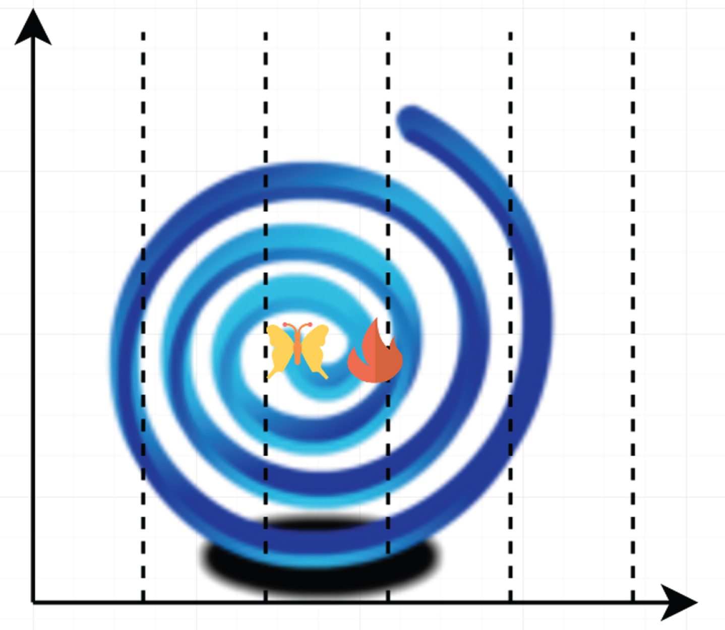
Geometric trajectory diagram of moths catching flames.

Abandoning flame behavior. As mentioned above, the flame is the optimal solution searched by the moth in the iterative process. The moth can approach one or more flames, and each moth approaches multiple flames to prevent local optimization and algorithm stagnation. During the iteration process, all the better flames in the parent and offspring are kept and sorted according to the size of the flame fitness value. In addition, flames with poor fitness values are discarded to reduce the number of flames adaptively, and finally converge to 1. This avoids the moth from losing the local optimal solution during the position update, so that the moth gradually moves to the flame with better fitness value and speeds up the later convergence speed.

F_{num} = round (N - l \cdot \frac{N - l}{T})

(8) In the above formula, F_num is the number of adaptive flame reduction: l is the current iteration number; N is the maximum number of flames: T is the maximum iteration number.

The algorithm terminates. When the flame fitness value reaches a predetermined standard or the number of iterations reaches the maximum number of iterations, the algorithm stops and outputs the spatial position and fitness value of the flame.

In view of the large number of seepage pressure monitoring model parameters, the MFO algorithm can be applied to solve the seepage pressure monitoring model coefficients. Each dimension of the moth matrix represents the parameters of the corresponding seepage pressure monitoring model, and the candidate solution flame position of the MFO algorithm is the undetermined seepage pressure monitoring model coefficient. When the moths are constantly approaching the flame, the error of the seepage pressure monitoring model is also continuously reduced. When the error is reduced to the desired value, the optimal flame position is output, that is, the model construction is completed.

4 Basic principles of CCMFO algorithm

Both the moth and the flame in the MFO algorithm are search factors for the optimization problem. The moth is the candidate solution of the problem to be solved and the position is constantly updated, and the flame is the best position currently searched in the iterative process of the moth. This kind of optimization strategy can explore the unknown search space as much as possible without giving up the optimal solution. However, when solving the parameter coefficients of the osmotic pressure model, due to the large number of dimensions set by the moths, the artificial moths approach the undetermined solution with a single spiral trajectory, which limits the variation of the moth population to a certain extent. In the solution of the coefficient problem of the seepage pressure monitoring model with multiple local optimal solutions, when the artificial moth has achieved a higher degree of optimization in some dimensions, it gives up the search for better values in the whole dimension, which causes the algorithm to be unable to find the global optimum flame when solving high-dimensional problems and fall into the local optimum. The golden mean solution generated by the vertical and horizontal crossover algorithm and the dominant solution generated by the parental competition enter the screening mechanism together to retain the global optimal flame position. On the one hand, this cross-over mechanism can effectively prevent local optimal moths from continuously iterating into their offspring, and on the other hand, it increases the advantages of global optimal moths in the iterative process. Moreover, the vertical and horizontal crossover algorithm improves the diversity of moth populations to reduce search blind spots, quickly transfers the position information of moths in the population with higher solution accuracy, retains the ability of moths to develop new positions, and effectively improves the overall solution accuracy of the algorithm. Through comparative tests with MFO, DE, and PSO algorithms, it is found that the CCMFO algorithm can improve the accuracy of the solution and the stability of the algorithm when solving high-dimensional complex function problems.

Horizontal crossing is an arithmetic crossing between two different moths in the same dimension in a moth population. Before crossover, all moths must be paired randomly without repetition, and then the same dimension of the paired moths must be crossed arithmetic. If we assume that the moth M_i and the moth M_j are paired, the horizontal crossover formula is: ${\begin{matrix} M_{hc} (i, d) = | c_{1} \cdot M_{id} - M_{jd} | \cdot e^{bt} \cdot cos (2 π t) + M_{id} \\ M_{hc} (j, d) = | c_{2} \cdot M_{jd} - M_{id} | \cdot e^{bt} \cdot cos (2 π t) + M_{jd} \end{matrix}$ (9)

In the formula, c₁, c₂, t ∈ [- 1, 1], and b = 1. Among them, M_hc (i, d) and M_hc (j, d) are the flame solutions of the offspring generated by the parent artificial moth M_i and the parent artificial moth M_j crossing on the d-th dimension, respectively.

In the above formula, it can be observed that the moths search in the hypercube space formed by the crosswise cross. The hypercube takes the parent moths M_i and M_j as the diagonal vertices, and the size is half of the population, and new moth individuals are more likely to be generated in the hypercube. In addition, the progeny moths are produced at the periphery of the space with a small linear decreasing probability, which increases the possibility of the moths to explore the external information of the hypercube, and reduces the search blind area of artificial moths to enhance the global search ability of the algorithm. Finally, the offspring moths are compared with the parent moths through a competition mechanism, and the better moth position is selected as the flame.

Longitudinal crossing

Longitudinal crossing is the crossing operation between two different dimensions of the same moth. In the seepage pressure monitoring model, the physical meanings of the vertical dimensions are not the same. In order to prevent overflow caused by the different value ranges between the two dimensions, it is necessary to ensure that the two dimensions of the vertical cross operation are consistent. Therefore, the data needs to be normalized. crossing is the crossing operation between two different dimensions of the same moth. In the seepage pressure monitoring model, the physical meanings of the vertical dimensions are not the same. In order to prevent overflow caused by the different value ranges between the two dimensions, it is necessary to ensure that the two dimensions of the vertical cross operation are consistent. Therefore, the data needs to be normalized.

At the same time, only one dimension is updated each time the flame catching of longitudinal crossing, which can effectively make the one dimension that is trapped in the local optimal dimension get rid of the stagnant state without destroying other normal dimensions. We perform the longitudinal crossing operation on the d₁ and d₂ dimensions of moth M_i to generate the d₁-th dimension offspring. The formula for longitudinal crossing is: $M_{vc} (i, d_{1}) = | c \cdot M_{id 1} - M_{id 2} | \cdot e^{bt} \cdot cos (2 π t) + M_{id 1}$ (10)

In the above formula, c, t ∈ [- 1, 1], and b = 1. Among them, M_vc (i, d₁) is the flame solution of the offspring generated by the artificial moth M_i in its d₁-th and d₂-dimensions crossed vertically to update the d₁-dimension.

When the swarm intelligence optimization algorithm is solving multi-dimensional problems, it is often unable to search for the global optimal individual because some dimensions reach better values. This kind of stagnant population iteration is called falling into the local optimal. The seepage pressure monitoring model tends to fall into the local optimum during the population iteration process due to many parameters. Therefore, integrating the longitudinal crossing into the MFO algorithm can effectively prevent the algorithm from falling into the local optimum. Moreover, the longitudinal crossing mutation method can produce a mean value, which effectively prevents the algorithm from selecting the optimal moth in individual dimensions to enter the offspring and abandoning the global optimal individual. In addition, the probability of longitudinal crossing occurs at [0.2, 0.8], which helps to get rid of the local optimum, and then make the population evolve towards the global optimum. After crossover, it is also compared with its parent moths, and the best ones are retained in the parent population. The vertical and horizontal crossover algorithm makes up for the spatial search ability lost by the competition mechanism due to the pursuit of convergence accuracy, while maintaining the diversity of the population without destroying the individual peacekeeping moths that may be better.

The crisscross optimization algorithm can increase the diversity of moth populations and randomly generate more moderate solutions to find the global optimal solution. In order to make the generated moth individuals more diverse, the cubic mapping method in the chaos algorithm is applied to the CCMFO algorithm. The moth performs a vertical and horizontal cross operation, and the initial value of the parameter t is a random value between [- 1, 1] and not 0. Subsequently, the value of t is generated by the cube map based on the previous generation solution, and the calculation formula of the chaos operator is: $t_{n + 1} = 4 t_{n}^{3} - 3 t_{n}, t \in [- 1, 1]$ (11)

The multiple regression model is an important method in the regression model. Influencing factors can be obtained and quantified, thereby determining the relationship and extent of the influence of each influencing factor on the dependent variable. We use x₁, x₂, ⋯ , x_m to represent m independent variables, and Y to represent dependent variables. Then, the established multiple linear regression model can be expressed as: $y = β_{0} + β_{1} x_{1} + β_{2} x_{2} + \dots + β_{m} x_{m} + ɛ$ (12)

In the formula, ɛ is a random error and β₀, β₁, β₂, ⋯ , β_m is m + 1 unknown parameters.

For practical problems with n sets of observation data, the regression model can be expressed as: ${\begin{matrix} y_{1} = β_{0} + β_{1} x_{11} + β_{2} x_{12} + \dots + β_{m} x_{1 m} + ɛ_{1} \\ y_{2} = β_{0} + β_{1} x_{21} + β_{2} x_{22} + \dots + β_{m} x_{2 m} + ɛ_{2} \\ ⋮ \\ y_{n} = β_{0} + β_{1} x_{n 1} + β_{2} x_{n 2} + \dots + β_{m} x_{nm} + ɛ_{n} \end{matrix}$ (13)

Its matrix form is: $y = X β + ɛ$ (14)

In the above formula: $y = (\begin{matrix} y_{1} \\ y_{2} \\ ⋮ \\ y_{n} \end{matrix})$ (15) $X = (\begin{matrix} 1 & x_{11} & x_{12} & \dots & x_{1 m} \\ 1 & x_{21} & x_{22} & \dots & x_{2 m} \\ ⋮ & ⋮ & ⋮ & ⋱ & ⋮ \\ 1 & x_{n 1} & x_{n 2} & \dots & x_{nm} \end{matrix})$ (16) $β = (\begin{matrix} β_{0} \\ β_{1} \\ β_{2} \\ ⋮ \\ β_{m} \end{matrix})$ (17) $ɛ = (\begin{matrix} ɛ_{1} \\ ɛ_{2} \\ ⋮ \\ ɛ_{n} \end{matrix})$ (18)

The parameter estimation of the multiple regression equation adopts the conventional least square method (OLS). Using this estimation method to estimate regression parameters needs to satisfy the following basic assumptions.

A₀ model setting assumption (linear assumption)

This is not a statistical assumption, but a model setting. This assumption requires that the conditional mean of Y is a linear function of all independent variables X: $E (y | x) = X β$ (19)

In the above formula, Y is a column vector of n × 1 composed of observations of dependent variables, x is a matrix of n × p composed of observations of independent variables, and p < n.

That is to say, the conditional expectation of Y under X can be expressed as a linear combination of X, and this conditional expectation is the regression equation. The model requires that X′X must be a non-singular matrix.

A₁ orthogonal hypothesis

We assume that the error term matrix ɛ is not related to each x vector in X. In other words, $Cov (X, ɛ) = 0$ (20)

When the first column of the X matrix is all 1, the above equation is equivalent to: $E (ɛ) = 0$ (21) $E (X^{'} ɛ) = 0$ (22)

This assumption ensures that the least squares estimation of regression model parameters is unbiased.

A₂ independent and identical distribution assumption

This assumption is for the error terms of the overall regression model, requiring them to meet the conditions of mutual independence and the same distribution. Specifically,

Independent distribution: each error term ɛ_i is independent distribution, namely: $Cov (ɛ_{i}, ɛ_{j}) = 0, i \neq j$ (23)

Homoscedasticity: $Var (ɛ_{i}) = σ_{i}^{2} = σ^{2}, i = 1, 2, \dots, n$ (24)

In matrix form, these two properties can also be expressed as: $Var (ɛ | X) = σ^{2} I$ (25)

In the above formula, I is the unit matrix of n × n order.

Gauss-Markov Theorem shows that if the assumptions of A₁ and A₂ are satisfied, the regression parameter estimate b obtained by the least square method will be the best linear unbiased estimate among all the estimates.

Linear estimated value refers to the estimated value θ that can be expressed as a linear function of the dependent variable, namely: $θ = \sum_{i = 1}^{n} w_{i} y_{i}$ (26)

w_i can be a function of the independent variables in the sample.

Under the assumption of A₁, the unbiased estimate b of the regression parameters can be obtained by using the least square method, that is $E (b) = β$ (27)

Since there may be many linear unbiased estimates, it is necessary to use the validity criteria to select the best estimate.

In the case of satisfying A₂, according to the Gauss-Markov theorem, it can be proved that the estimation result of the least square method is the smallest variance among all linear unbiased estimates.

A₃ normal distribution assumption

On the basis of the A₂ assumption, this assumption further requires that ɛ_i obey a normal distribution N (0, σ²). The assumption of normal distribution makes the least square estimation can be understood as the maximum likelihood estimation-the best unbiased estimation.

However, the normal distribution assumption is mainly used for statistical testing of the least squares estimated values of the regression parameters, and this issue needs special attention only in the case of small samples. For large samples, according to the central limit theorem, even if the error term does not satisfy the normal distribution, the estimated value of the regression parameter can still be inferred statistically.

5 Model building

The model uses a deep denoising autoencoder to denoise the original input data set and then conduct unsupervised layer-by-layer learning and training. Moreover, the model minimizes the error between the original input data set and the unsupervised training output data to obtain the feature vector of the original input data set. Then, the model uses support vector regression as the predictor of the final output layer of the model, and uses the acquired feature vectors of the original data set as the input feature vectors of support vector regression for prediction. The structure of the DDAE-SVR deep neural network model is shown in Fig. 2:

Fig. 2

Model network structure.

The evaluation sample data set is divided into training data set and test data set. The training data set is input into the model mentioned in this chapter for training. Afterwards, by adjusting the number of hidden layers of the model, the optimization algorithm and other parameters, as well as the relevant parameters of support vector regression, a stable and optimal model is obtained to optimize the prediction efficiency. Finally, the test data set is input to verify the effectiveness of the model in evaluating teaching quality. The flow chart of DDAE-SVR deep neural network model to evaluate the teaching quality of colleges and universities is shown in Fig. 3:

Fig. 3

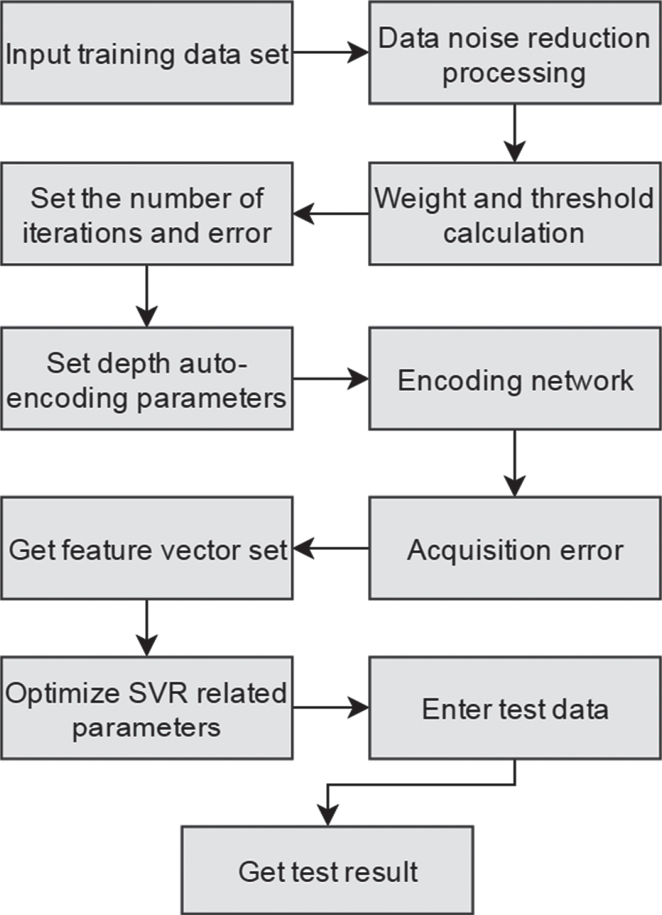
The flow chart of DDAE-SVR deep neural network model to evaluate the teaching quality of colleges and universities.

The quality evaluation model for classroom teaching is shown in Fig. 4.

Fig. 4

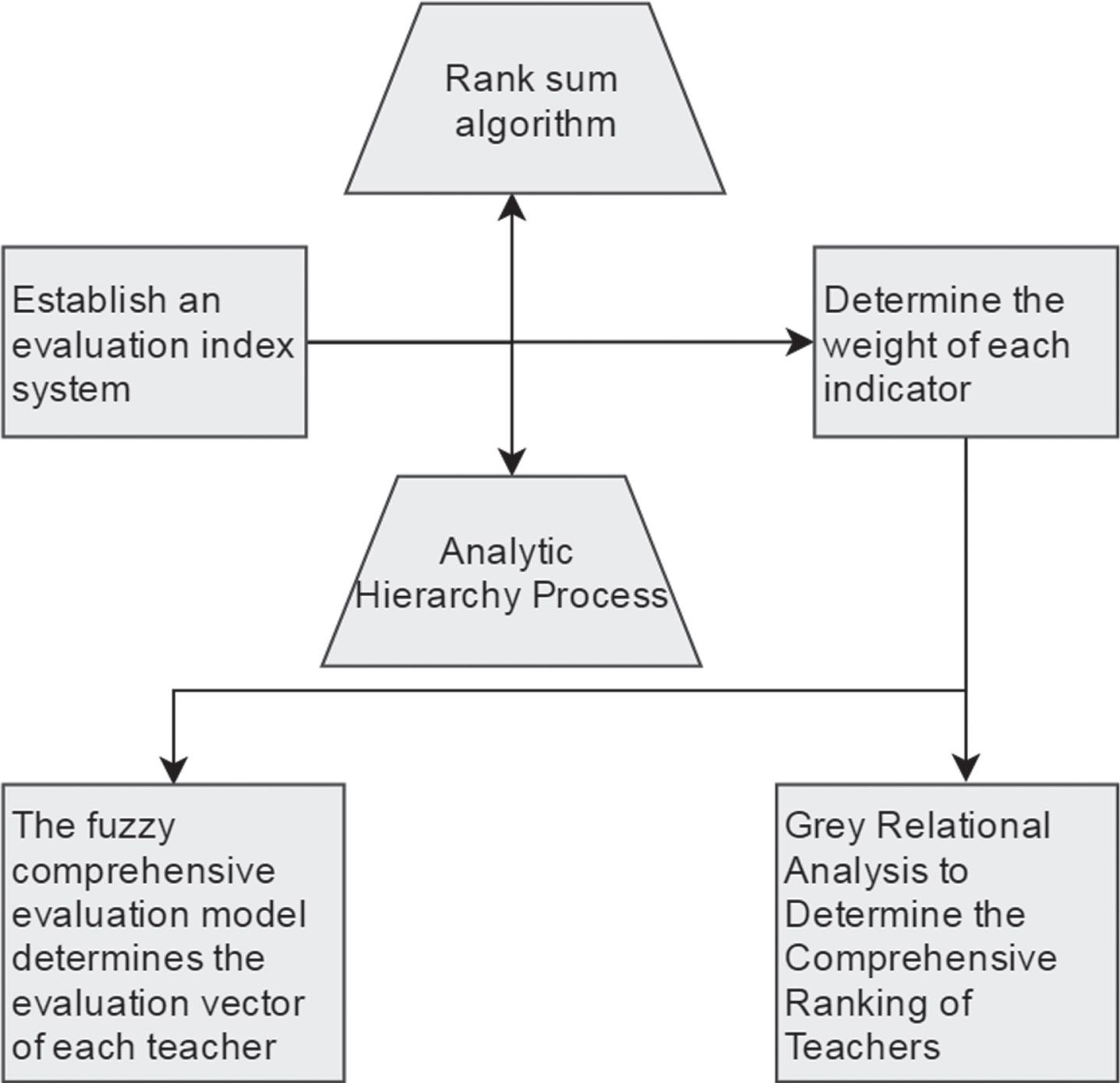
Classroom teaching quality evaluation model.

The teacher’s teaching quality evaluation model is shown in Fig. 5.

Fig. 5

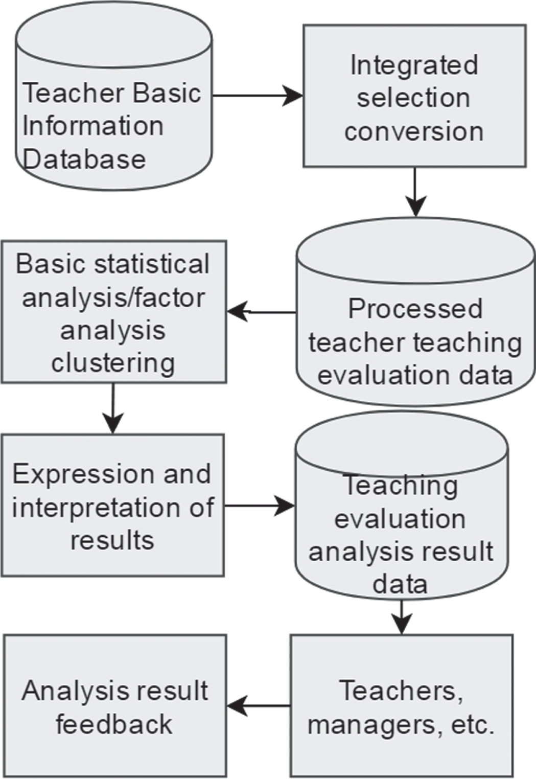
Teacher’s teaching quality evaluation model.

The model is trained through the neural network model. After repeated training cycles, the actual output value of the network and the target expected value reach the expected error. This process is the entire training network error reaches the required minimum value. After repeated iterative calculations of the network, if the error is less than the allowable minimum value, the training process of the network stops. The training process flowchart is as follows:

The data set format is (x1,x2,......,x23,y), and there are 1788 sample data in total. Among them, the data used to evaluate the teaching process of teachers with students as the main evaluation body is used as the input value of the evaluation model. Because the expected output value of the target is very important to the verification of the model, a comprehensive score based on the evaluation of multiple lecture records by the teachers of the teaching supervision group is used as the expected output value of the model. Through the analysis of the data set, the sample data with high evaluation, low evaluation and inconsistent with the facts are removed, and finally 1578 sample data are obtained. Then, normalization preprocessing is performed on the finally obtained data samples. The purpose is to improve the computational efficiency of the BP neural network model. The sample data after normalization is shown in Table 1 and Fig. 7.

Table 1

Examples of sample data after normalization

	1	2	3	4	5	6	7	8	... ...
1	0.85	0.88	0.86	0.85	0.82	0.90	0.92	0.90	... ...
2	0.93	0.84	0.88	0.77	0.86	0.77	0.86	0.91	... ...
3	0.75	0.72	0.85	0.74	0.83	0.76	0.79	0.66	... ...
4	0.94	0.78	0.94	0.83	0.76	0.95	0.87	0.78	... ...
5	0.85	0.76	0.77	0.92	0.90	0.85	0.88	0.76	... ...
6	0.83	0.88	0.94	0.81	0.84	0.83	0.88	0.85	... ...
7	0.85	0.86	0.83	0.89	0.85	0.94	0.87	0.88	... ...
8	0.94	0.80	0.90	0.77	0.81	0.77	0.86	0.76	... ...
9	0.92	0.89	0.85	0.94	0.84	0.80	0.76	0.89	... ...
10	0.89	0.86	0.85	0.78	0.94	0.80	0.79	0.79	... ...
11	0.84	0.84	0.79	0.73	0.69	0.72	0.66	0.66	... ...
12	0.80	0.84	0.91	0.82	0.94	0.79	0.85	0.91	... ...
13	0.82	0.81	0.83	0.92	0.92	0.76	0.83	0.95	... ...
14	0.91	0.77	0.80	0.80	0.83	0.89	0.91	0.80	... ...
15	0.82	0.85	0.85	0.80	0.86	0.81	0.69	0.65	... ...
16	0.87	0.85	0.84	0.93	0.79	0.84	0.89	0.82	... ...
17	0.86	0.92	0.88	0.86	0.82	0.86	0.90	0.82	... ...
18	0.73	0.85	0.79	0.80	0.79	0.85	0.82	0.69	... ...
19	0.87	0.86	0.89	0.85	0.95	0.92	0.94	0.87	... ...
20	0.78	0.80	0.86	0.90	0.90	0.79	0.83	0.82	... ...
21	0.68	0.87	0.89	0.84	0.76	0.65	0.80	0.78	... ...
22	0.81	0.89	0.83	0.84	0.89	0.88	0.77	0.95	... ...
23	0.81	0.86	0.84	0.80	0.81	0.75	0.82	0.79	... ...
y	0.87	0.91	0.94	0.83	0.90	0.85	0.92	0.86	... ...

Fig. 6

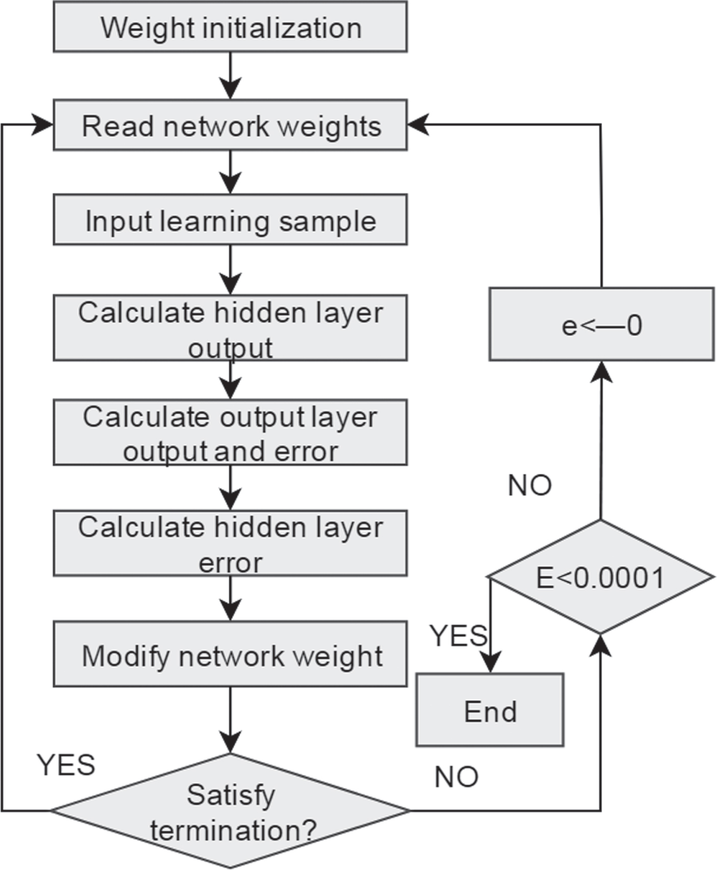
Flow chart of network training process.

Fig. 7

Statistical graph of sample data after normalization.

In order to verify the effectiveness of the model proposed in this article in the evaluation of teaching quality in universities. This paper uses the standard BP neural network model to input the traditional data set (model1) and the new data set (model2), and the self-applicable BP neural network model to input the new data set to construct three neural network models for the evaluation of university teaching quality. Moreover, this article runs 10 experiments for each model to get the average value. At the same time, two models based on decision tree algorithm and support vector machine are constructed to evaluate teaching quality, and the other four models constructed are compared with the models proposed in this chapter. The experimental results are shown in Table 2 and Fig. 8.

Table 2

Comparison of operating effects of different models

	MSE	Forecast accuracy rate (%)	Training time (s)	Number of iterations
model1	60.42	93.10	12.08	5000
model2	52.85	93.72	12.25	5000
decision-tree	52.24	93.61	0.03	—–
SVM	25.45	95.81	0.13	—–
MFO	24.43	95.89	0.33	74

Fig. 8

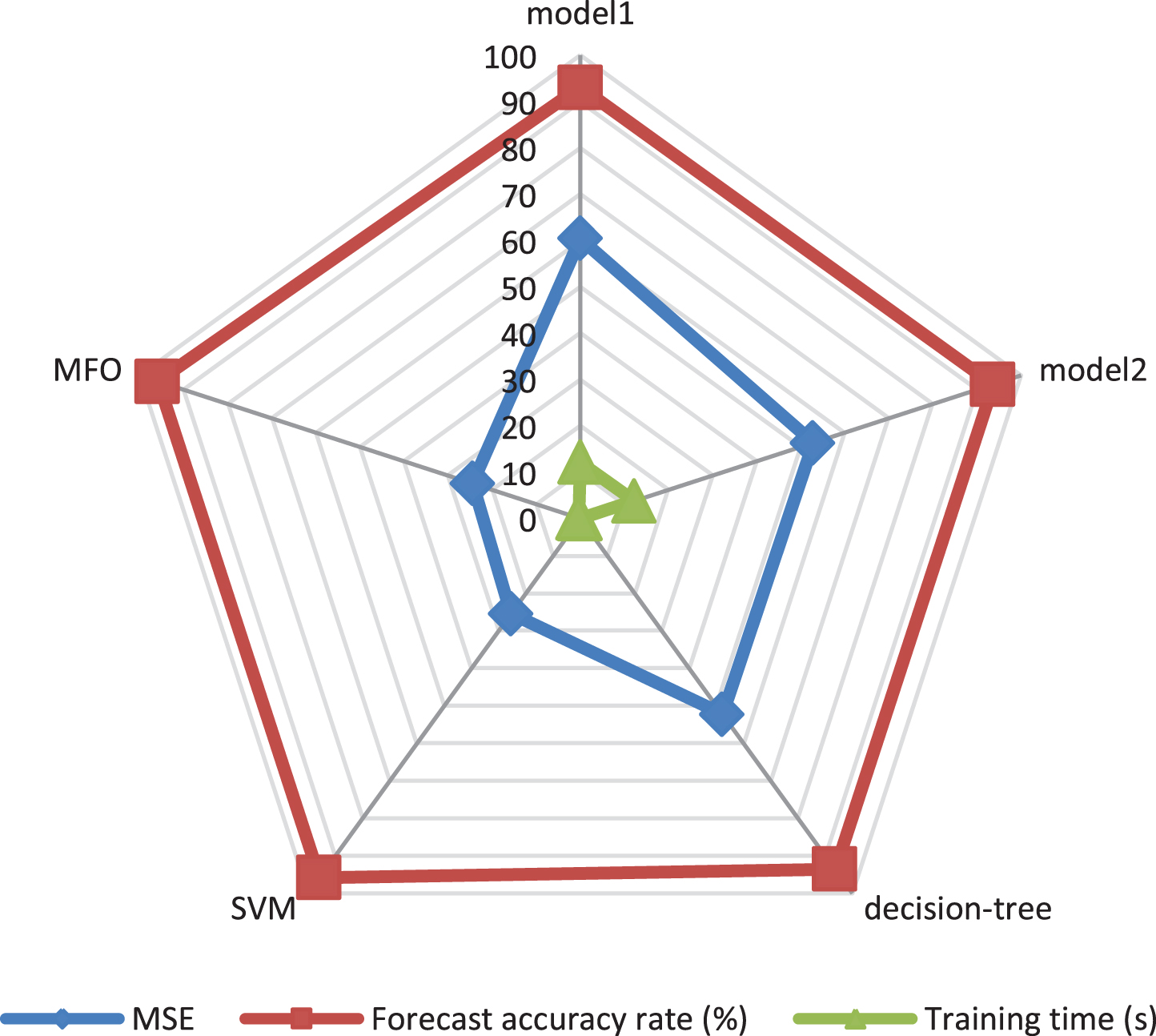
Comparison diagram of effects of different models.

It can be seen from the above chart that the model constructed in this article is more effective than other models.

6 Conclusion

Teaching quality is the core content of educational competitiveness, the lifeline of higher education, especially higher vocational colleges, and the foundation and prerequisite for the sustainable development of education. Improving the quality of teaching is the core of improving the quality of education in universities, especially higher vocational colleges. In particular, it is necessary to improve the teaching quality of teachers’ courses. The MFO algorithm imitates the horizontal positioning principle of moth-catching flames in nature, uses a logarithmic spiral to simulate the path of moths toward the flame, and inverts the pending parameters in the mathematical model. Moreover, this paper adds vertical and horizontal algorithms and chaos operators on this basis. The crisscross algorithm allows different moth individuals and the same moth to perform cross calculations with different operational dimensions to increase the diversity of moth populations, so that moths in the search space can traverse the entire search space as much as possible to find a better solution. At the same time, the introduction of chaos operator is conducive to artificial moths to jump out of the local optimal solution during chaos development. In addition, the model constructed by the MFO algorithm is used to evaluate the effect of teaching quality, and the performance of the model is analyzed through experiments. The research results show that the model constructed in this paper has certain effects.

References

Sieg

, Flachsenberg

and Rarey

, In need of bias control: evaluating chemical data for machine learning in structure-based virtual screening, Journal of Chemical Information and Modeling 59(3) (2019), 947–961.

Thabtah

and Peebles

, A new machine learning model based on induction of rules for autism detection, Health Informatics Journal 26(1) (2020), 264–286.

Narudin

F.A.

, Feizollah

, Anuar

N.B.

, et al., Evaluation of machine learning classifiers for mobile malware detection, Soft Computing 20(1) (2016), 343–357.

Bzdok

and Meyer-Lindenberg

, Machine learning for precision psychiatry: opportunities and challenges, Biological Psychiatry: Cognitive Neuroscience and Neuroimaging 3(3) (2018), 223–230.

Itu

, Rapaka

, Passerini

, et al., A machine-learning approach for computation of fractional flow reserve from coronary computed tomography, Journal of Applied Physiology 121(1) (2016), 42–52.

Jayasinghe

, Lee

G.M.

, Um

T.W.

, et al., Machine learning based trust computational model for IoT services, IEEE Transactions on Sustainable Computing 4(1) (2018), 39–52.

Rajkomar

, Dean

and Kohane

, Machine learning in medicine, New England Journal of Medicine 380(14) (2019), 1347–1358.

Ward

, Agrawal

, Choudhary

, et al., A general-purpose machine learning framework for predicting properties of inorganic materials, npj, Computational Materials 2(1) (2016), 1–7.

Amershi

, Cakmak

, Knox

W.B.

, et al., Power to the people: The role of humans in interactive machine learning, Ai Magazine 35(4) (2014), 105–120.

10.

Coley

C.W.

, Barzilay

, Jaakkola

T.S.

, et al., Prediction of organic reaction outcomes using machine learning, ACS Central Science 3(5) (2017), 434–443.

11.

Linhares

R.N.

, Alcântara

C.M.G.

, Gonçalves

E.Á.

, et al., Teaching Evaluation by Teachers from Brazil and Portugal: A Comparative Analysis, American Journal of Educational Research 5(5) (2017), 546–551.

12.

Huang

, Analysis and Design of University Teaching Evaluation System Based on JSP Platform, International Journal of Education & Management Engineering 7(3) (2017), 43–50.

13.

Liu

and Chen

, Research on Fuzzy Comprehensive Evaluation in Practice Teaching Assessment of Computer Majors, International Journal of Modern Education & Computer Science 7(11) (2015), 12–19.

14.

Zhou

, Li

and Sun

, Teaching performance evaluation by means of a hierarchical multifactorial evaluation model based on type-2 fuzzy sets, Applied Intelligence 46(1) (2016), 1–11.

15.

Porozovs

, Liepniece

and Voita

, Evaluation of the Teaching Methods Used in Secondary School Biology Lessons, Nephron Clinical Practice 7(1) (2015), 60–66.

16.

Oliveros

M.A.

, García

and Valdez

, Evaluation of a Teaching Sequence Regarding Science, Technology and Society Values in Higher Education, Creative Education 6(16) (2015), 1768–1775.

17.

Cerón

M.S.

and del Sagrario Corte Cruz

F.M.

, The Evaluation of Teaching: Some Consequences for Latin America, Revista Mexicana De Investigacion Educativa 20(67) (2015), 1233–1253.

18.

, Li

and Ge

, Application of Data Mining in the Colleges’ in-Class Teaching Quality Evaluation System, Journal of Computers 10(3) (2015), 166–175.

19.

Angell

and Tewell

, Teaching and Un-Teaching Source Evaluation: Questioning Authority in Information Literacy Instruction, Communications in Information Literacy 11(1) (2017), 95–121.

20.

Jiang

and Wang

, Evaluation of Teaching Quality of Public Physical Education in Colleges Based on the Fuzzy Evaluation Theory, Journal of Computational and Theoretical Nanoence 13(12) (2016), 9848–9851.

21.

Royal

, A Guide for Making Valid Interpretations of Student Evaluation of Teaching (SET) Results, Journal of Veterinary Medical Education 44(2) (2016), 1–7.

22.

Garofalo

, Mota-Moya

, Munday

, et al., Total Extraperitoneal Hernia Repair: Residency Teaching Program and Outcome Evaluation, World Journal of Surgery 41(1) (2017), 1–6.