Simulation of athlete gait recognition based on spectral features and machine learning

1 Introduction

With the rapid development of computer technology, the way of human-computer interaction has changed dramatically. From the early reliance on keyboard and mouse input methods, to the later popular touch screen interaction, to the currently popular face recognition and voice recognition, etc., in the process of updating and iterating the entire human-computer interaction technology, the interaction method becomes more intelligent. At the same time, people’s requirements for user experience in human-computer interaction are also increasing. The significance of studying gesture interaction is that it has a wide range of application scenarios, such as VR, intelligent robot interaction, smart home, unmanned driving, and intelligent assisted driving systems. It is of great significance to the development of artificial intelligence and to facilitate people’s lives [1].

In the context of the rapid development of artificial intelligence, several branches have emerged, among which the direction of human motion recognition [2] is particularly popular. It can be used in different fields such as film and television production, human-computer interaction, game entertainment, and motion analysis. We can use human motion recognition to capture people’s movement trajectories and record their movement data, use 3D animation to simulate human movement for film and television production, and somatosensory games also realize game interaction by recognizing human movement poses. It is also widely used in intelligent monitoring. The main principle is: embedding human body gesture recognition technology into the video server, using algorithms to judge and identify the dynamic objects in the monitoring scene, and extract the key information. When a pedestrian or a vehicle behaves abnormally, it can promptly alert the user. For example: For elderly people living alone in ordinary families or hospital patients, we can respond to the sudden and unexpected situation of falling by monitoring [3] equipment, so as to promptly feedback to others and automatically open the alarm system. In a public place where the population density is relatively concentrated, if only rely on manual participation in management, not only can not be comprehensive supervision, but also cause a waste of human resources, so intelligent monitoring is the best choice [4].

The implementation of the above applications is the epitome of the motion capture technology [5], and this technology is widely used in the movie “Avatar”. The motion capture technology was invented based on Fisher’s image tracing, and it has been produced in the animation production process. By playing each frame of static video in the video clip to simulate the feeling of the animated character in the virtual world, the animation script is generated by formulating the action, and the sensor ball inside can roughly locate the position of the joint point of the human skeleton. The current motion capture technology is developed on this basis. The motion capture system is generally composed of two parts: software and hardware. The hardware part includes transmitting and receiving sensors and signal transmission equipment. The software part includes functional modules such as spatial positioning, system setting, and data processing.

In this paper, based on machine learning and spectral feature technology, different recognition technologies for athletes are studied, and computer vision technology is applied to sports to promote the development of computer vision technology.

2 Related work

The literature [6] innovatively proposes a single target tracking problem (Support Vector Tracking, SVT) based on the SVM algorithm. In order to train the SVM classifier offline, it uses a large number of data samples. At the same time, the classifier is used as a priori observation model to distinguish the foreground and background. However, there are some limitations, such as no online update mechanism, which leads to SVT can only be applied to certain specific tracking, cannot be well adapted to changes in the target in real time. Moreover, its application in real scenes is very limited. The literature [7] used Correlation Filters (CF) for the first time in the field of target tracking and made great improvements. The main idea of the correlation filter of the MOSSE algorithm is:the higher the similarity between the target in the image and the initial target, the greater the response. The TLD tracking algorithm is proposed by in the literature [8]. The TLD tracking algorithm adds the tracking module and the detection module to the learning process, and constantly updates the positive and negative sample libraries in the learning module for subsequent tracking, which makes the tracking results more stable and reliable. The biggest drawback of the above two methods is that the size of the target is not considered. During a tracking process, changes in the size of the target will cause the tracker to either learn redundant features (become smaller) or only learn some features (become larger), which will cause tracking drift and failure. The appearance of the literature [9] (target tracking reference data set) sets a specific evaluation standard for target tracking, so that people can intuitively evaluate the performance of a tracker. The literature [10] proposed the SAMF tracking algorithm. The contribution of this article mainly has two points(1)The article expands a single feature into multiple features, including HOG features, CN (color space) and grayscale fusion features; (2) The article uses the scale pool method to realize the adaptive tracking of the target, and at the comparison stage, the target in the candidate area is calculated at seven scales and compared with the target of the previous frame. Moreover, its maximum response value serves as the target in the current frame. However, the multi-feature fusion of this article is very simple and is just a simple vector superposition, and there are many redundant features. Moreover, the candidate area is only compared with the target in the previous frame. Once the target tracking in the previous frame fails, the subsequent tracking effect will be affected. The algorithm provides a theoretical basis for the application of multi-feature fusion in target tracking and confirms that the candidate regions can be compared with the target in the previous frame to filter the results. With the emergence and success of deep learning, deep learning methods have become one of the attractive research methods. To some extent, deep learning has triggered a scientific revolution in the data age. Convolutional neural networks have demonstrated outstanding performance on a variety of visual tasks, such as: image classification, target detection, and semantic segmentation. Due to the excellent feature modeling ability of deep learning methods, in the field of target tracking, deep learning methods have been promoted and achieved great success. At present, the more successful trackers are all discriminative trackers based on deep learning. In the work of [11], the author put forward a new idea differently. This article does not treat VGG-Net as a classified black box but uses the features of different layers in VGG-16 for tracking. Moreover, the feature selection through the BP (back propagation) regression model makes the features sparseand makes the tracking more accurate and robust. However, it defaults that the candidate area of the next frame of the picture is the Gaussian distribution centered on the result position of the previous frame. In the case of practical application, the fast movement of the tracking target, camera offset, and target loss will affect the accuracy, stability and success rate of the tracker. In addition, this work only considers the convolution features of the tracking target, which are not interpretable and insufficiently targeted. If other effective tracking features can be added, such as: color histogram, HOG feature, etc., there will be better tracking effect. In 2017, CSR-DCF [12] tracking algorithm and CFNet_conv2 [13] tracking algorithm were proposed on CVPR (Conference on Computer Vision and Pattern Recognition). The former uses the color model of the foreground and background to construct the target matrix to limit the spatial domain of the filter and gives a solution method. At the same time, the weighting coefficients of different channels are constructed using the response graph information of different channels, that is, the reliability coefficient of the channel. However, the algorithm does not use convolution features, which limits the performance of the tracker. At the same time, the algorithm proves that the color module of the foreground and background can be used for target tracking. The latter paper is based on the improvement of convolutional neural networks, and it mainly adds new layers and derives forward and reverse formulas. Moreover, it is also an end-to-end network, which makes the network have good performance under shallow features and makes the overall network lightweight and faster. However, this article only considers convolution features and ignores other valid features, so there is still room for improvement. The article [22] addresses the issue such as enormous volume of bigdata and come up with the concept of SmartBuddy to form brilliantly and savvy environment utilizing human practices and human elements. The article [23] talks almost the development of coordinated non-cyclic chart for video coding calculations for movement estimation in parallel reconfigurable computing frameworks. Moreover, the partitioning algorithm plays a major part to speed up the video processing. The article [24] dealt exploiting IoT and BigData Analytics utilizing Hadoop environment in genuine time situations. Execution of IoT-based Smart City is accomplished by the above-mentioned processes. The article [25] centers around IoT and its significant job in sophisticating the human practices and endeavors. This paper additionally managed the assortment of different information from different assets that are associated with the web. The literature [26] addresses the different issues within the field of vehicle communication with the recommendation of a common bound together and scattered range detecting demonstrate. The application of the shared cognitive paradigm minimizes struggle and different obscure problems [27, 28].

3 Kalman filter

The literature [14] proposed a linear filter for discrete time-varying linear systems, which is an optimized autoregressive filter that can estimate the state of a dynamic system from a series of incomplete and noise-containing measurements. Kalman filter technology is relatively mature in engineering applications, and its process is described by a series of recursive mathematical formulas. These formulas provide an efficient and computable method to estimate the state of the process and minimize the estimated mean square error.

As a method of signal processing, the Kalman filter can be used to estimate the state quantity of the systemand simultaneously process the state equation and measurement equation of the system. Among them, the state equation describes the law of the system state changes with time, and the measurement equation describes the relationship between the measured physical quantity and the state. We assume that x _k is the state of the system at time k, x_k+1 is the state of the system at the next time, u _k is the control amount of the system at time k, and w _k is the process noise of the system. Then, the state equation of the discrete control process system can be expressed by a linear stochastic differential equation, as shown in formula (1). x k + 1 = A k x k + B k u k + w k(1)

In the formula, A _k is the state transition matrix of the system from time k to timek + 1, and B _k is the transition matrix of the control quantity relative to the state.

If z_k+1 represents the system measurement value at time k + 1, and v_k+1 represents the measurement error at time k + 1, the measurement equation can be expressed as follows [15]: z k + 1 = H k + 1 x k + 1 + v k + 1(2)

In the formula, H_k+1 is the observation matrix at time k + 1, which can be used to express the function mapping relationship between the state quantity and the measured value.

We assume that the process noise and measurement noise of the system are both white noise with an average value of 0, and the two are uncorrelated and satisfy: E { w k w k T } = Q δ jk E { v k v k T } = R δ jk δ jk = { 1 if j = k 0 if j ≠ k(3)

In the above formula, Q and R are the covariance matrix of process noise w and measurement noise v, respectively. In statistics and probability theory, each element of the covariance matrix is to calculate the covariance between different dimensions, which reflects the transfer of uncertainty between vector elements at various times. The covariance matrix plays an important role in the process of Kalman filter recursively solving the optimal estimated value. The subsequent Kalman filter derivation process is realized by the system state covariance matrix combined with the linear minimum mean square error estimation method [16].

The basic operation process of Kalman filtering can be divided into three stages: prediction, correction and update. In the prediction stage, the state equation of the system needs to be constructed first, as shown in formula (4). x k + 1 - = A k x k + B k u k + w k(4)

Unlike formula (1), x k + 1 - is used in formula (4) to indicate the predicted state value rather than the non-actual state value. Correspondingly, the state transition matrix according to the state equation can realize the prediction of the state covariance matrix, as shown in formula (5). P k + 1 - = A k P k A k T + Q(5)

In the formula, A _k is the state transition matrix in formula (4), Q is the process noise covariance matrix in formula (3), P _k is the state covariance matrix determined at time k, and P k + 1 - is the state covariance matrix predicted at time k + 1.

After the prediction phase is completed, there are two known state values: one is the current state prediction value just obtained, and the other is the current observation value [16]. There is some inaccuracy between the two, so they need to be combined to correct. In the correction phase, a key quantity in the Kalman filter is introduced first, namely the Kalman gain. The calculation formula of Kalman gain is as follows: K k + 1 = P k - H k + 1 T ( H k + 1 P k - H k + 1 T + R ) - 1(6)

In the above formula, H _k is the observation matrix in formula (2), is the observation noise covariance matrix in formula (3), and P k - is the state covariance matrix predicted at time k.

Next, the Kalman gain is applied to the estimated value and the observed value, and the final reliable state value can be obtained, as shown in formula (7) [17]. x k + 1 = x k + 1 - + K k + 1 ( z k + 1 - H k + 1 x k + 1 - )(7)

According to formula (7) and formula (6), it can be found that the Kalman gain can determine whether the final result is closer to the predicted value or the observed value by weighing the size of the predicted state covariance matrix and the measured noise covariance matrix. The smaller the covariance of the observed noise, the greater the Kalman gain, and the final result is closer to the observed value. However, the larger the covariance of the observed noise, the smaller the Kalman gain, and the final result is closer to the predicted value. This compromise idea enables the Kalman filter to use the observed values to modify the predicted state values, even if the observed values and predicted values are in different dimensions [18].

Finally, before starting the next Kalman filtering process, the current state value covariance matrix needs to be updated for subsequent iterations. The formula is as follows: P k + 1 = P k + 1 - - K k + 1 H k + 1 P k + 1 -(8)

Improving its accuracy by calibrating the sensor is a necessary task for realizing the body area network. Calibration refers to the process of solving the relationship between the two by comparing the standard input and the sensor output, and the relationship among them is often a linear relationship, so it can be regarded as the process of solving the coefficient and offset. Different sensors have different calibration methods. The following describes the calibration methods of the three sensors used in this article.

(1) Gyro calibration

Zero drift is an important type of error in the gyroscope. The long-term accumulation of this error will greatly affect the accuracy of the attitude calculation. By default, if the three-axis gyroscope is stationary, the reading output of all three axes should be 0dps. Due to the unstable voltage and the device itself, the sensor signal fluctuates up and down, but the average value should still be close to 0dps. Therefore, when calibrating the zero-point drift of the gyroscope, the data at the moment of rest of the gyroscope can be collected for a long time, and the average value of the three axes can be obtained as the calibration parameter of the zero-point drift [19].

(2) Accelerometer calibration

As a type of observation value of the attitude calculation method, the accuracy of the acceleration signal will affect the accuracy of the attitude quaternion, so it needs to be calibrated before use. This article adopts a convenient and easy way to find the zero drift of each axis of the accelerometer and the proportional relationship between them. First, the sensor node needs to be adjusted so that the accelerometer has readings on the X axis and no readings on the Y and z axes. Next, the accelerometer rotates smoothly along the z axis, and the data of the x and y axes are formed into the coordinate (x, y) of the point on the two-dimensional rectangular coordinate system. Then, a pattern similar to that shown in Fig. 1 can be obtained [20].

OPEN IN VIEWER

Fig. 1

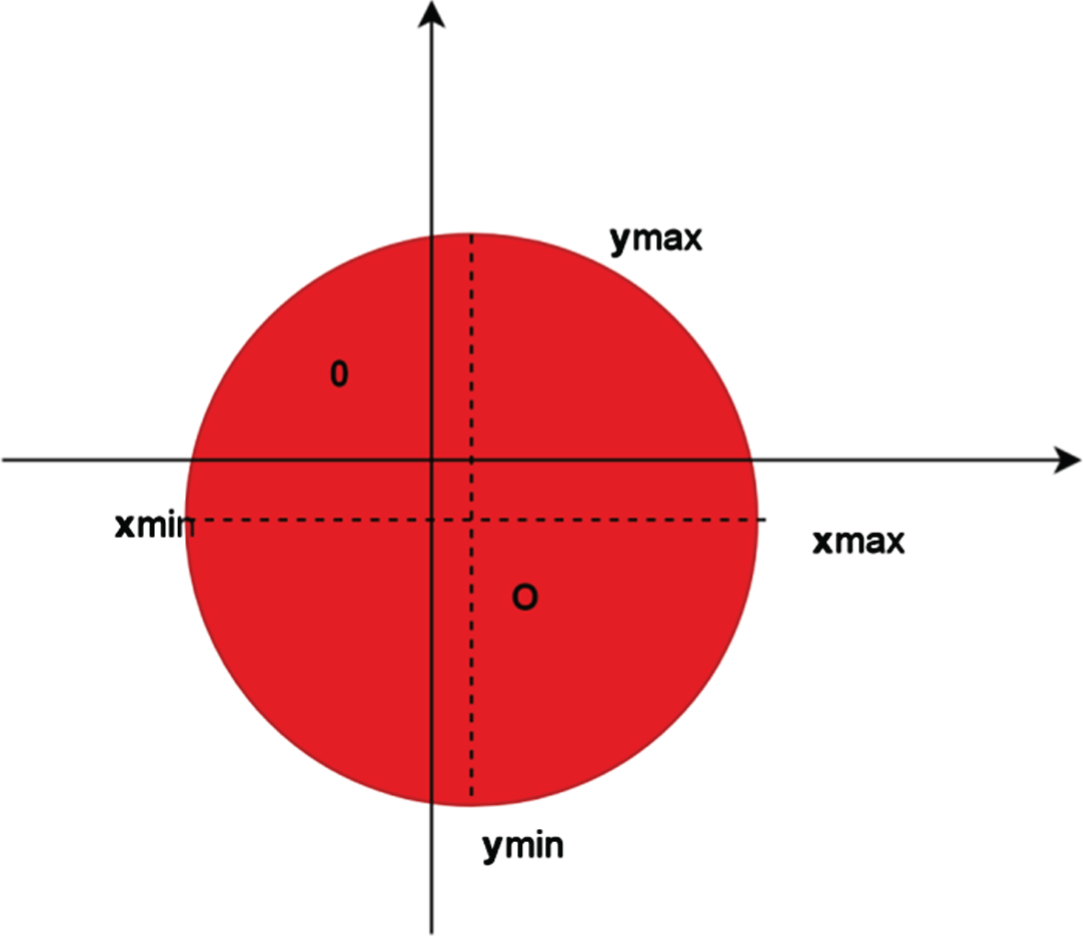
Schematic diagram of accelerometer calibration

If it is assumed that the accurate value of acceleration is(x′, y′, z′), and there is a linear relationship between the accurate value and the measured value, the relationship can be expressed by formula (9) as follows: x ′ = a x · ( x + b x ) y ′ = a y · ( y + b y ) z ′ = a z · ( z + b z )(9) x ′ 2 + y ′ 2 = g ′ 2(10)

Among them,a _x a _y a _z is the coefficient relationship between the x, Y, and z axis readings of the sensor and the true value, and b _x b _y b _z is the zero drift of the X, Y, and Z axes, respectively. Since the sensor rotates smoothly along the Z axis, it is not affected by external forces except gravity acceleration. Therefore, in the case of accurate sensor readings, the readings on the x and y axes should satisfy formula (10), where the symbol g represents the acceleration of gravity [21].

By bringing formula (9) into formula (10), the relationship between the actual acceleration value and the acceleration of gravity can be obtained as shown in formula (11). a x 2 ( x + b x ) 2 + a y 2 ( y + b y ) 2 = g 2(11)

It can be seen from formula (11) that the formula is an ellipse expression, the x coordinate of the center point is the opposite number of the zero drift of the accelerometer X axis, and the Y coordinate of the center point is the opposite number of the zero drift of the accelerometer Y axis. According to the calculation formula of the geometric ellipse center point and Fig. 1, the formulas for b _x and b _y can be obtained as follows: b x = - ( x max + x min ) / 2 b y = - ( y max + y min ) / 2(12)

In the formula, x_max and x_min are the maximum and minimum values of the accelerometer on the x-axis, and y_maxandy_min are the maximum and minimum values of the accelerometer on the y-axis. At the same time, according to the geometrical ellipse length and radius calculation formula, the solution formulas for a _x and a _y are as follows: a x = 2 g / ( x max - x min ) a y = 2 g / ( y max - y min )(13)

Through the above method, the X-axis and Y-axis outputs of the accelerometer can be calibrated. Similarly, the attitude of the sensor node can be adjusted so that the accelerometer has data on the Z axis and no data on the X and Y axes, and we use the X and Y axes as the axis to perform rotation, and use the above calculation method to obtain the Z axis calibration formula.

(3) Electronic compass calibration

Magnetic field strength is another important observation value of the sensor node’s attitude calculation, and its calibration method is similar to that of acceleration. In different environments, there is a certain change in the magnetic field. Therefore, for gait behavior recognition devices, electronic compass calibration needs to be performed more frequently, while gyroscopes and accelerometers often only need to be calibrated once. Taking into account the practical requirements, we should try our best to simplify the calibration process and cost. This article uses a calibration method to draw the ‘8’ character. Before the sensor node works, the node is placed in the correction mode, and the word “8” is drawn in the space more than 3 times in the hand, which enables each axis of the gyroscope to be horizontal to the magnetic field direction within a short time. Next, the calibration step is similar to the accelerometer calibration, and the zero drift and error coefficient are obtained from the maximum and minimum values of each axis. After the calibration is completed, the node status is set to the acquisition mode, and the calibration parameters obtained in the calibration mode can be used to achieve the calibration without reprogramming the hardware.

After the dynamic time domain segmentation method is used to divide the time series data into segments, it is necessary to extract valuable features from the segmented data as the basis for dividing the gait category. In general, features can be defined as the abstraction of data, and the significance of feature extraction is to obtain key attributes that can accurately describe the original data. In this paper, a heuristic feature extraction method is adopted. By observing and analyzing the waveforms of lower leg angular velocity signals and behaviors of various leg movements in daily life, 20 kinds of features that are considered to reflect the differences between leg movements are selected. According to different description objects, these features can be divided into waveform features and behavioral features. When one-leg gait behavior is detected, the system will automatically extract all waveform features and behavioral features for use in subsequent gait classification phases. The following uses the right calf as an example to introduce the selected features and the calculation method of each feature value.

Waveform characteristics can be used to reflect the fluctuation of the signal over a period of time, which is mainly reflected in the distribution of extreme points. By observing the calf angular velocity, it can be found that there are certain rules for the fluctuation of various gait waveforms, and these rules can be reflected by the size of the extreme points P, IC and TC and the numerical relationship between the extreme points. In order to verify this finding, this study takes 100 samples of walking, running, going upstairs, and going downstairs, respectively, and obtained the extreme point angular velocity values for each gait. Figure 2 shows the distribution of peak angular velocity obtained from various gait samples. It can be seen from the figure that the peak value of the running sample is significantly larger than that of other gaits, and the peak range is approximately 460dps   590dps. The peak ranges of walking and going downstairs are 300dps–410dps and 270dps–360dps, respectively, and there is most overlap between the two ranges. The peaks of going upstairs are generally distributed between 180dps and 280dps, which are relatively small in the four types of gait, but still have a small part of the peak range of going downstairs. Therefore, according to the magnitude of the peak value, the running motion can be effectively identified from the four types of gait samples in the figure. However, it is difficult to accurately distinguish other types of actions, especially for walking and downstairs, which has little classification reference value. In addition, by comparing the difference in angular velocity between IC and TC, the differences between walking, running, going upstairs, and going downstairs can also be found. Figure 3 shows the numerical distribution of the angular velocity difference between IC and TC for various gaits. Among them, the difference between IC and TC for running and going downstairs is positive, and the difference for running is relatively large, but the distribution is more scattered. Contrary to going downstairs, the difference in going upstairs is negative. However, the difference in walking on the ground cannot determine the sign of the sign, and its size is distributed between –80dps and 80dps. It can be seen that the difference between the angular velocity of IC and TC can effectively distinguish the upstairs and downstairs movements, so it can also be used as a criterion to judge the gait category.

OPEN IN VIEWER

Fig. 2

The distribution of wave crests for walking, running, going upstairs, and going downstairs

OPEN IN VIEWER

Fig. 3

The distribution of angular velocity difference between IC and TC for walking, running, going upstairs, and going downstairs

In addition to the above features, using the angular velocity values of the three extreme points of P, IC and TC can obtain more waveform features. First, the angular velocity of the three extreme points is taken as the basic waveform characteristics, which are denoted by ω _p  (k) ω _IC  (k) and ω _TC  (k), respectively. Among them, the variable k represents the order of gait. By making the difference between the above three characteristics, the following three characteristics can be obtained: Diff IC , TC ( k ) = ω IC ( k ) - ω TC ( k )(14) Diff P , IC ( k ) = ω P ( k ) - ω IC ( k )(15) Diff P , TC ( k ) = ω P ( k ) - ω TC ( k )(16) In addition to the difference, the magnitude relationship between the extreme points can also be reflected in the form of ratio, as shown in formulas (17), (18), (19): Ratio IC , P ( k ) = ω IC ( k ) / ω P ( k )(17) Ratio TC , P ( k ) = ω TC ( k ) / ω P ( k )(18) Ratio IC - PC ( k ) = Diff IC , TC ( k ) / ω P ( k )(19)

These characteristics can reflect the violent degree of angular velocity waveform and the distribution of extreme points during the fluctuation process, which helps to distinguish different types of gait behavior.

The behavioral characteristic can be used to describe the kinematics of gait. For humans, these features are easy to perceive, easier to understand and accept than waveform features, and are important attributes for determining the type of gait. Considering that a complete gait behavior is completed by both legs, the experiment samples the angular velocities of the left and right legs simultaneously. The subgraphs a to d in Fig. 4 show the changes of the left and right calf angular speeds of the four types of movements of squatting, jumping, walking and running, respectively. It is not difficult to see that in the process of squatting and jumping, the distribution of the extreme points of the two curves in the time domain is very similar, while the distribution of the extreme points in walking and running is more scattered. In order to describe the timing relationship between the extreme points, P (k) IC (k) and TC (k) are used to indicate the moments of the three extreme points of the right calf waveform in the k-th gait cycle, and P′ (k) IC′ (k)andTC′ (k) represent the moments of the three extreme points of the left calf waveform in the k-th gait cycle.

OPEN IN VIEWER

Fig. 4

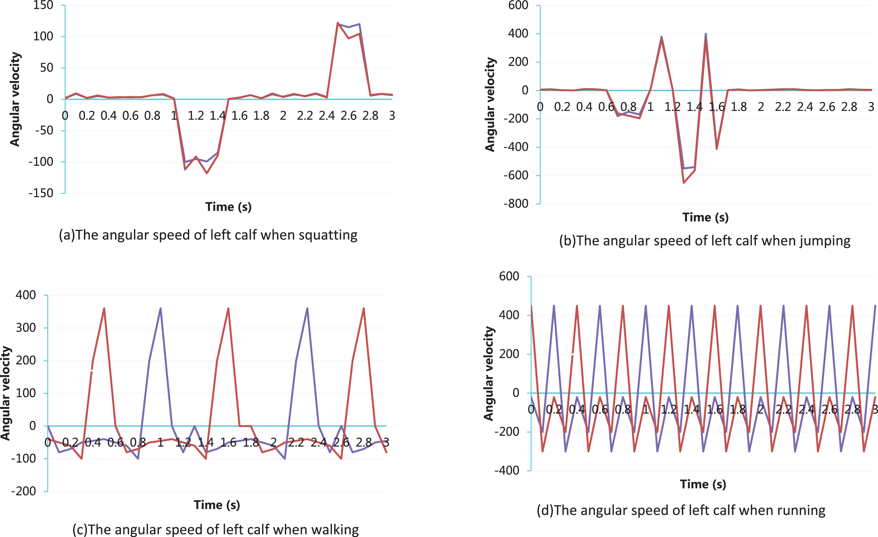
The angular velocity waveforms of legs during walking, running, squatting and jumping

For squatting and jumping, the movements of the left and right calves are almost synchronized, so the time sequence of each extreme point cannot be determined. However, through this feature, the time interval Time_P′,P (k)between P (k) and P′ (k) can be obtained to express the degree of synchronization of the movement of the legs. Time P ′ , P ( k ) = | P ′ ( k ) - P ( k ) |(20)

Unlike squatting and jumping, due to the alternating swing of legs during walking and running, the extreme points will appear in a specific time sequence. If it is assumed that the movement of the left leg occurs before the right leg, the timing relationship between the extreme points during walking and running is shown in formula (21) and formula (22), respectively: IC ′ ( k ) < P ′ ( k ) < TC ′ ( k ) < IC ( k ) < P ( k ) < TC ( k ) < IC ′ ( k + 1 )(21) IC ′ ( k ) < P ′ ( k ) < IC ( k ) < TC ′ ( k ) < P ( k ) < IC ′ ( k + 1 ) < TC ( k )(22)

The reason is that when the heel of the swinging leg touches the ground during walking, the toe of the rear leg has not left the ground, so that both feet keep in contact with the ground at the same time. However, during running, when the heel of the swinging leg touches the ground, the toe of the rear kick has already left the ground, so there is no time period when both feet touch the ground at the same time. Therefore, the time difference Time_IC,TC′ (k) between IC (k) and TC′ (k) can be obtained according to formula (23), which represents the time when both feet support the ground at the same time. When the Time_IC,TC′ (k) symbol is positive, it means that the current action is walking, otherwise, it means that the current action is running. Time IC , TC ′ ( k ) = | IC ( k ) - TC ′ ( k ) |(23)

In addition to the features that can be used to describe the alternation of the legs, the timing parameters of the extreme points can also be used to obtain the time parameters of gait behaviors such as walking, running, and going upstairs and going downstairs: Gait cycle time: GC ( k ) = IC ( k + 1 ) - IC ( k )(24)

Single foot support time: Stance ( k ) = IC ( k + 1 ) - TC ( k )(25)

Single foot swing time: Swing ( k ) = TC ( k ) - IC ( k )(26)

Single foot stride time: Stride ( k ) = TC ( k ) - TC ′ ( k )(27)

It should be pointed out that the above parameters have no actual physical meaning for squatting and jumping. However, these parameters can reflect the details of the action process and can be used as an effective indicator for quantitative analysis of gait behavior, thus helping to identify gait behavior.

In addition, the swing angle θ _thigh of the thigh and the swing angle θ _shank of the calf can also be obtained by using Equations (28) and (29). Among them,ω _thigh  (t) and ω _shank  (t) represent the angular velocity of the thigh and calf at time t, respectively. θ thigh ( k ) = ∫ IC ( k ) TC ( k ) ω thigh ( t ) dt(28) θ shank ( k ) = ∫ IC ( k ) TC ( k ) ω shank ( t ) dt(29)

At the same time, the attitude quaternion of the waist node can be used to reflect the rotation of the waist during the movement. Q _IC represents the quaternion at the time of IC, Q _TC represents the quaternion at the time of TC, and the quaternion describing the rotation of the waist is represented by quat = (w, x, y, z). The relationship between the three can be obtained as follows: quat · Q IC = Q TC(30)

Next, the quaternion quat can be obtained using the Gaussian elimination method, and then the rotation angle θ _waist of the waist in the Y-axis direction of the three-dimensional Cartesian coordinate system within the swing stage can be obtained according to the quaternion conversion Euler angle formula. θ waist ( k ) = arcsin ( 2 ( w · y - z · x ) )(31)

Using the above calculation method, the waist rotation angle within the gait cycle can be obtained. This parameter can be used to describe the change of the human body orientation during the movement.

Finally, an indicator is used to indicate which side of the lower leg the currently calculated feature value corresponds to.

So far, all the features and calculation methods have been introduced. After detecting the occurrence of a gait behavior, the above-mentioned features can be obtained from each sensor data, and a feature vector is formed as a sample representing the current gait. It should be noted that when the human body transitions from a static state to a motion state, no other actions occur before the first leg action, so that some features related to the other leg cannot be obtained, which led to the inconsistency of the feature vector dimensions of the gait samples and ultimately affected the accuracy of the classification results. In addition, for continuous gait, such as walking, running, going up and down stairs, the behavior of the first leg movement is not obvious compared to the subsequent movements. Although the two belong to the same action type, there may be a large difference in the distribution of values for the same feature. To this end, according to the time sequence of gait, it is divided into the initial gait and the subsequent gait, which represent the first gait behavior of the human body transition from static to the motion state and the gait behavior in the process of movement. Moreover, two types of gait are considered separately in the subsequent gait classification stage.

In order to obtain the training sample set and the test sample set required by the experiment, this paper samples the gait behavior of the tester, extracts the feature vector corresponding to each leg action through periodic division, and adds a category label to it. In the process of collecting training samples, in order to ensure that each type of sample is sufficient, the experiment samples different types of actions separately, and requires the tester to complete the specified number of actions. In the process of collecting test samples, the tester moves according to a certain route, during which various types of movements are completed alternately, and there is no limit to the number of movements to simulate the actual activities of people in daily life. The tester in this article is a track and field athlete who volunteered to participate in the test. In this article, the testers were asked to perform 100 gait movements, and a total of 100 people are tested to count the categories of these gait movements. After that, the traditional image recognition technology (IRT), neural network technology (NNT) and the gait recognition technology (TAOTA) proposed by this study are compared in pairs.

The first is to compare the traditional image recognition technology with the gait recognition technology proposed by this study. The results are shown in Table 1 and Fig. 5.

OPEN IN VIEWER

Fig. 5

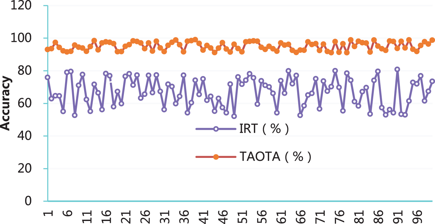
Comparison diagram of accuracy of gait recognition between IRT and TAPTA

It can be seen from Table 1 and Fig. 5 that the gait recognition technology proposed in this study has a high accuracy rate of 90% for athletes’ gait recognition and has a strong stability. However, the accuracy of traditional image recognition technology is less than 80%, and the stability is insufficient.

It can be seen from Table 2 and Fig. 6 that the gait recognition technology proposed by this study has a high accuracy rate of 90% for athletes’ gait recognition and has a strong stability. However, the accuracy rate of neural network technology is between 70% and 85%, and the stability is insufficient.

OPEN IN VIEWER

Fig. 6

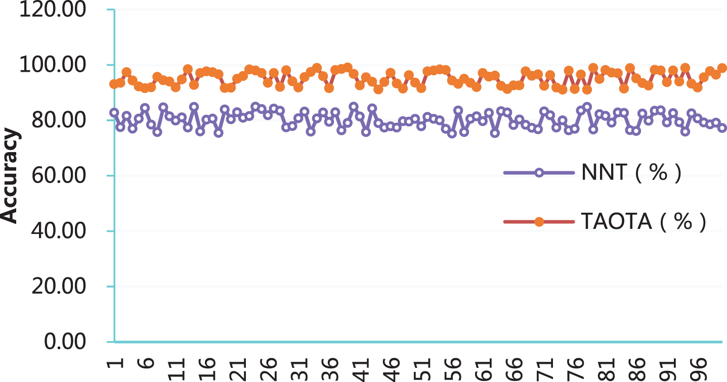
Comparisondiagram of accuracy of gait recognition between NNT and TAPTA

Through the above experimental research, we can see that the gait recognition technology proposed by this study has a certain effect and can be applied to practice.

In order to study the athlete’s gait recognition technology, this paper proposes the athlete’s gait recognition technology based on spectral features and machine learning. The method in this paper can detect the occurrence of leg movements in real time based on the calf angular velocity signal, and accurately divide the gait cycle, reduce the influence of the behavior-independent signals on the recognition process, thereby improving the accuracy of gait recognition results, which provides a new idea for the study of gait behavior recognition. By analyzing the behavior of the leg movements such as walking, running, turning, squatting, jumping, going upstairs and going downstairs and the signal waveform of the sensor, this paper extracted 20 heuristic features as the attribute set for describing gait samples. Finally, the performance of the algorithm in this paper is analyzed through experimental research. The comparison results show that the method proposed by this paper has improved the number of recognition action types and accuracy and has certain advantages from the perspective of computation and scalability. Moreover, the gait recognition method proposed in this paper can achieve stable and satisfactory recognition effect for different people’s gait actions.