Route planning of intelligent bridge cranes based on an improved artificial potential field method

Abstract

The artificial potential field method is usually applied to the path planning problem of driverless cars or mobile robots. For example, it has been applied for the obstacle avoidance problem of intelligent cars and the autonomous navigation system of storage robots. However, there have been few studies on its application to intelligent bridge cranes. The artificial potential field method has the advantages of being a simple algorithm with short operation times. However, it is also prone to problems of unreachable targets and local minima. Based on the analysis of the operating characteristics of bridge cranes, a two-dimensional intelligent running environment model of a bridge crane was constructed in MATLAB. According to the basic theory of the artificial potential field method, the double-layer artificial potential field method was deduced, and the path and track fuzzy processing method was proposed. These two methods were implemented in MATLAB simulations. The results showed that the improved artificial potential field method could avoid static obstacles efficiently.

Keywords

Artificial potential field intelligent bridge crane path planning static environment

1 Introduction

Bridge cranes are the most commonly used lifting and transportation machinery in modern production. They are widely used in factories, warehouses, and material fields. However, determining how to achieve intelligent transportation in environments that are not comfortable to enter (such as unmanned storage, landfill disposal, and nuclear waste handling) is a problem that must urgently be solved by scientists [1 –3]. To realize the intelligent operation of a bridge crane, path planning technology must be studied.

Path planning technology has two main research directions: sensor detection technology and obstacle avoidance algorithms [4]. Obstacle avoidance algorithms have two main research focuses: global static and local dynamic path planning [5]. In global static path planning, all the information about the environment is known, and in local path planning, some or no information about the working environment is known. The global path planning is based on all the environmental information entered in advance or detected by various sensors to form an environment map, after which path planning is carried out based on the environment map.

2 Artificial potential field theory

The classical artificial potential field theory [6] was proposed by the American scientist Khatib in a 1985 IEEE conference paper. His original intention was to use obstacle avoidance planning for robotic arms or mobile robots. The central idea of the classical artificial potential field method is to regard the movement of the robot in the working environment as a kind of motion in an artificially designed virtual force field. The robot will be subjected to a kind of “gravitational force” generated by the target position and a “repulsive force” generated by the obstacle. The movement direction of the robot can be controlled by the resultant force of the robot [7].

3 Establishing a two-dimensional intelligent bridge crane operating environment model

The running speeds of the gantry and trolley of the universal bridge crane typically are in the range of 80–135 and 40–60 m/min, respectively.

Since the setting of the environment in this study was based on a square grid, the running speeds and acceleration of the gantry and trolley were the same. To improve the efficiency, the running speeds of the gantry and trolley were 1 m/s, and the acceleration was 0.5 m/s2.

Setting V = v = 1m/s and a = 0.5m/s² and using the following formulas: $t = \frac{V}{a}$ (1) $S_{1} = \frac{1}{2} {at}^{2}$ (2) $S_{2} = Vt - \frac{1}{2} {at}^{2}$ (3) where t the time spent on starting or braking (s), a is the acceleration of the gantry and trolley (m/s2), S₁ is the starting distance (m), and S₂ is the braking distance (m), it was concluded that t = 2s, S₁ = 1m, and S₂ = 1m.

Because 0.72 < S₁ <4 and 0.72 < S₂ <3, the set speed of the gantry and trolley was 60 m/min (1 m/s), and the acceleration was 0.5 m/s2, which met the braking requirements of the bridge crane. The lifted item was assumed to be a cube with a 1-m length, width, and height. To simplify the lifted item as a point mass in the grid, an appropriate side length of the grid was set, as follows:

$L = S_{1} + S_{2} + b = 3 m$ (4) where L is the grid side length (m) and b is the side length of the lifted mass (m). Therefore, we set the side length of the grid to 3 m.

The span of a bridge machine is usually 1.5-m smaller than the span of the plant in practice. Every 3-m increase is one class, with a range from 10.5 to 31.5 m. A non-standard span is used when the span exceeds 31.5 m. The span of the bridge crane was set to 31.5 m, the total width of the grid was 30 m, and the total length of the grid was 45 m.

The operating environment of the overhead crane is shown in Fig. 1. The circles indicate the obstacles. The difference in the radii of the circles indicates differences in the sizes of the obstacles. An obstacle of any shape can be surrounded by a circle on this plane, so a circular shape was selected for convenience. The positions, radii, and number of the circles were selected arbitrarily. The initial position of the weight was (0,0), and the target position was (10,15).

Fig.1

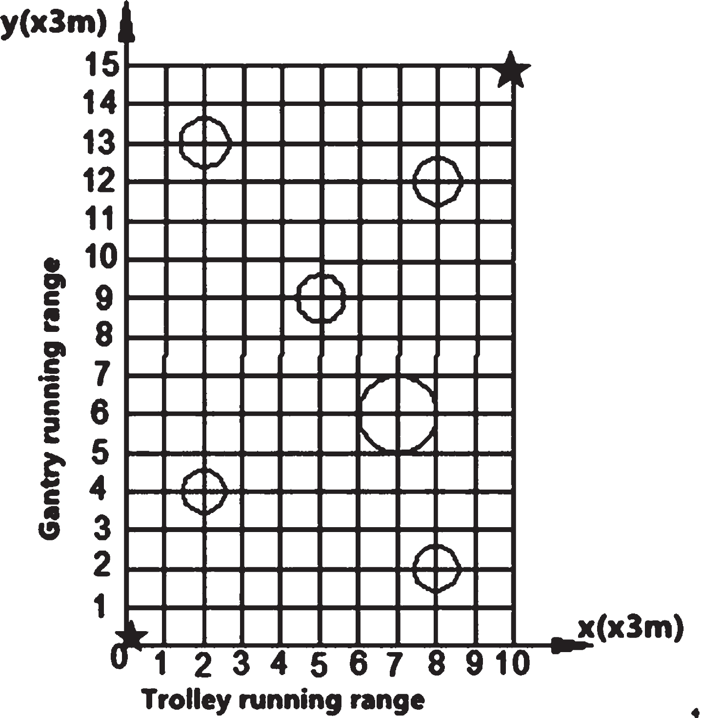
Operating environment of the bridge crane.

4 Improved artificial potential field method

For the problem of an unreachable target, in the repulsion potential field function, an item was added approximately at a distance equal to that between the weight and target position to ensure that when the weight was close to the target position, the gravitational and repulsion forces decreased simultaneously, minimizing the value of the potential field when the weight reached the target position.

As for the local minima problem, many researchers have conducted in-depth studies on path planning with artificial potential field method and proposed many different solutions, such as simulated annealing [8, 9], introduction of an escape force [10,11, 10,11], use of angle deviations [12, 13], and walking along the wall [14 –17].

To solve the problem of local minima, two methods are proposed: a double-layer artificial potential field method and a path and track fuzzy processing method.

4.1 Gravitational potential field function

The gravitational potential field function is defined as follows: $U_{att} = \frac{1}{2} {kd}_{wm}^{2}$ (5)

where U_att is the gravitational potential field function, k is the gravitational potential field gain coefficient, which is a constant k > 0, and d_wm is the Euclidean distance between the weight and the target position, the vector direction of which points from the weight toward the target position [18].

The mathematical expression of gravity is as follows:

$F_{att} = - grad (U_{att}) = {kd}_{wm} (\frac{\partial U_{att}}{\partial d_{wm}})$ (6)

4.2 Double-layer artificial potential field method

The repulsion potential field function is expressed as follows:

$\begin{matrix} U_{rep} = \\ {\begin{matrix} \frac{1}{2} η {(\frac{1}{d_{wn}} - \frac{1}{r_{n} + d_{0}})}^{2} d_{wm}^{β} & r_{n} < d_{wn} ⩽ r_{n} + λ d_{0} \\ \frac{1}{2} η {(\frac{1}{d_{wn}} - \frac{1}{r_{n} + d_{0}})}^{2} d_{wm}^{γ} & r_{n} + λ d_{0} < d_{wn} ⩽ r_{n} + d_{0} \\ 0 & r_{n} + d_{0} < d_{wn} \end{matrix} \end{matrix}$ (7) where U_rep is the repulsion potential field function, η is the repulsive potential field gain coefficient, which is a constant η > 0, d_wn is the Euclidean distance between the weight and the center of the obstacle, whose vector direction points from the center of the obstacle toward the weight, r_n is the radius of the obstacle circle, where each obstacle circle can be set with a different radius, d₀ is the maximum distance at which an obstacle affects the repulsive force of a heavy object, β is a constant 1 < β, γ is a constant 0 < γ < 1, and λ is a constant 0 < λ < 1.

The two parts of the repulsion function F_rep1 and F_rep2 are defined as follows:

$\begin{matrix} F_{rep 1} = \\ {\begin{matrix} η (\frac{1}{d_{wn}} - \frac{1}{r_{n} + d_{0}}) \frac{1}{d_{wn}^{2}} d_{wm}^{β} \frac{\partial U_{rep}}{\partial d_{wn}} & r_{n} < d_{wn} ⩽ r_{n} + λ d_{0} \\ η (\frac{1}{d_{wn}} - \frac{1}{r_{n} + d_{0}}) \frac{1}{d_{wn}^{2}} d_{wm}^{γ} \frac{\partial U_{rep}}{\partial d_{wn}} & r_{n} + λ d_{0} < d_{wn} ⩽ r_{n} + d_{0} \end{matrix} \end{matrix}$ (8)

$\begin{matrix} F_{rep 2} = \\ {\begin{matrix} \frac{β}{2} η {(\frac{1}{d_{wn}} - \frac{1}{r_{n} + d_{0}})}^{2} d_{wm}^{β - 1} \frac{\partial U_{rep}}{\partial d_{wm}} & r_{n} < d_{wn} ⩽ r_{n} + λ d_{0} \\ \frac{γ}{2} η {(\frac{1}{d_{wn}} - \frac{1}{r_{n} + d_{0}})}^{2} d_{wm}^{γ - 1} \frac{\partial U_{rep}}{\partial d_{wm}} & r_{n} + λ d_{0} < d_{wn} ⩽ r_{n} + d_{0} \end{matrix} \end{matrix}$ (9)

Letting d₀ = 2, r_n = 0.5, λ = 2, η = 1, β = 2, and $γ = \frac{1}{2}$ ,the formula is expressed as follows:

$F_{1} = {\begin{matrix} (\frac{1}{d_{wn}} - 0.4) \frac{1}{d_{wn}^{2}} d_{wm}^{2} & 0.5 < d_{wn} ⩽ 1.5 \\ (\frac{1}{d_{wn}} - 0.4) \frac{1}{d_{wn}^{2}} d_{wm}^{\frac{1}{2}} & 1.5 < d_{wn} ⩽ 2.5 \\ ∥ \end{matrix}$ (10)

$F_{2} = {\begin{matrix} {(\frac{1}{d_{wn}} - 0.4)}^{2} d_{wm} & 0.5 < d_{wn} ⩽ 1.5 \\ \frac{1}{4} {(\frac{1}{d_{wn}} - 0.4)}^{2} d_{wm}^{- \frac{1}{2}} & 1.5 < d_{wn} ⩽ 2.5 \\ ∥ \end{matrix}$ (11)

For d_wm = 2, d_wm = 4, and d_wm = 6, MATLAB was used to plot the two functions of F₁.

Based on the six curves in Fig. 2, if 1 〈 |d_wm| and d_wn has the same value, the function value of F1 in the interval d_wn ∈ (0.5, 1.5) is greater than that of F1 in interval d_wn ∈ (1.5, 2.5) [19]. There is a large gap in the function values between the two regions.

Fig.2

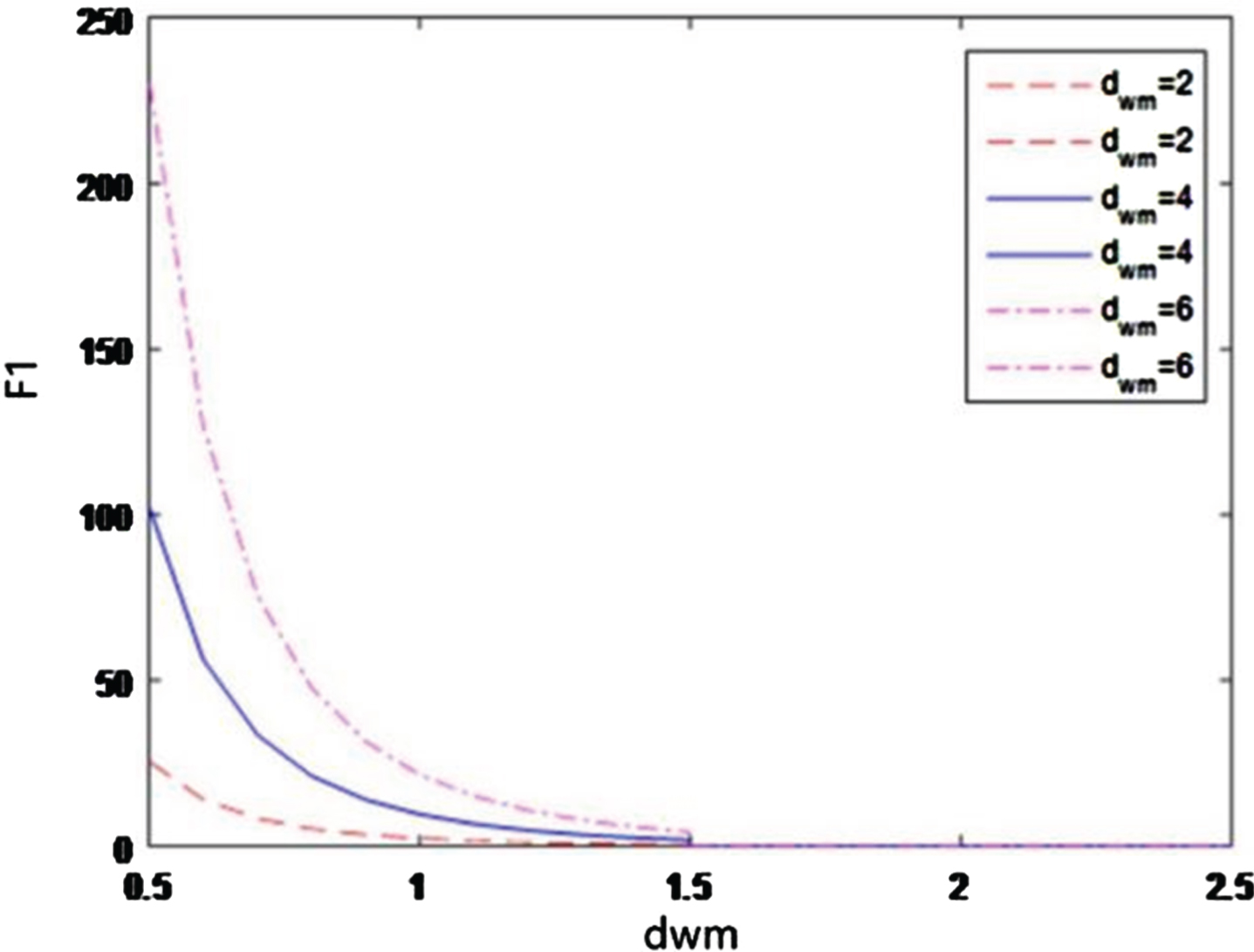
Plot of F₁.

For d_wm = 2, d_wm = 4, and d_wm = 6, MATLAB was used to plot the two functions of F₂.

Based on Fig. 3, when F_rep2 is 1 〈 |d_wm| and d_wn has the same value, its function values in interval d_wn ∈ (r_n, r_n + λd₀) must be larger those in interval d_wn ∈ (r_n + λd₀, r_n + d₀), and there was a large gap between the function values in these regions. This behavior is similar to that of F_rep1.

Fig.3

Plot of F₂.

For the double-layer artificial potential field method constructed in this paper, the repulsive force function is no longer a continuous function. The function is discontinuous, and gravity is located exactly at the discontinuity [20,21, 20,21]. In this case, the attraction and repulsion forces can never equal, and only two scenarios can occur: either the gravitational force is greater than the repulsion force (the weight reaches the outer layer of the repulsive potential field), or the repulsion force is greater than the gravitational force (the weight reaches the inner layer of the repulsion potential field).

When in the outer layer of the repulsive potential field, d_wn ∈ (r_n + λd₀, r_n + d₀). The force required to move the weight to the target position is greater than the force that causes the weight to move in the opposite direction, and thus, F_rep1 < F_att + F_rep2. When in the inner layer of the repulsive potential field, d_wn ∈ (r_n, r_n + λd₀). The force required to cause the weight to move to the target position is less than the force that causes the weight to perform the reverse motion, and thus, F_rep1 > F_att + F_rep2. Through the above analysis, the following formulas can be obtained:

$\begin{matrix} η (\frac{1}{d_{wn}} - \frac{1}{r_{n} + d_{0}}) \frac{1}{d_{wn}^{2}} d_{wm}^{β} > {kd}_{wm} + \frac{β}{2} η \\ {(\frac{1}{d_{wn}} - \frac{1}{r_{n} + d_{0}})}^{2} d_{wm}^{β - 1} r_{n} < d_{wn} ⩽ r_{n} + λ d_{0} \end{matrix}$ (12)

$\begin{matrix} η (\frac{1}{d_{wn}} - \frac{1}{r_{n} + d_{0}}) \frac{1}{d_{wn}^{2}} d_{wm}^{γ} < {kd}_{wm} + \frac{γ}{2} η \\ {(\frac{1}{d_{wn}} - \frac{1}{r_{n} + d_{0}})}^{2} d_{wm}^{γ - 1} r_{n} + λ d_{0} < d_{wn} ⩽ r_{n} + d_{0} \end{matrix}$ (13)

4.3 Fuzzy processing method for path trajectory

Letting the two-dimensional space coordinate of the weight in the operating environment of the bridge crane be (x, y) and the coordinate of the target position be (x_m, y_m), the line between the weight and the target position passes through the range of the repulsive potential field of an obstacle. The central coordinate of the obstacle is (x_z, y_z), the circle radius of the obstacle is r_z, and the maximum distance of the obstacle’s repulsive potential field is d₀. The slope of the line between the weight and the target position is k_m, where

$k_{m} = \frac{y_{m} - y}{x_{m} - x}$ (14)

The connection equation between the weight and the target position is as follows:

$\begin{matrix} k_{m} (x - x_{m}) = y - y_{m} \\ k_{m} x - y + (y_{m} - k_{m} x_{m}) = 0 \\ ∥ \end{matrix}$ (15)

The distance d from the obstacle to the connecting line between the heavy object and the target position is as follows:

$d = \frac{| k_{m} x_{z} - y_{z} + (y_{m} - k_{m} x_{m}) |}{\sqrt{k_{m}^{2} + 1}}$ (16)

As shown in Fig. 4, when d ∈ (1.1r_z, r_z + d₀), the weight can move forward along the line between the weight and the target position without being affected by the obstacle’s repulsive potential field. The reason the size range of d was set as d ∈ (1.1r_z, r_z + d₀) was not only to leave a gap between the heavy object and the obstacle to prevent their collision but also to make the heavy object move along the line without being affected by the repulsive force generated by the obstacle.

Fig.4

Schematic of the path trajectory fuzzy processing method.

5 Simulation

5.1 Simulation of classical artificial potential field method

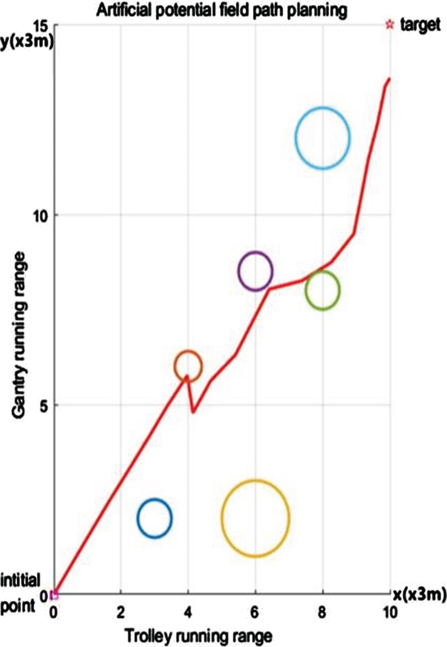
The first environmental examined was as follows: the starting point was (0, 0), the target point was (10, 15), the number of obstacles was 6, and the central coordinates were (3, 2; 4, 6; 6, 2; 6, 8.5; 8, 8; 8, 12), the radii of the obstacle circles were 0.5, 0.4, 1, 0.5, 0.5, and 0.8, and the number of iterations was 200. The other parameter values were as follows: k = 5, η = 10, d₀ = 3, and l = 1.

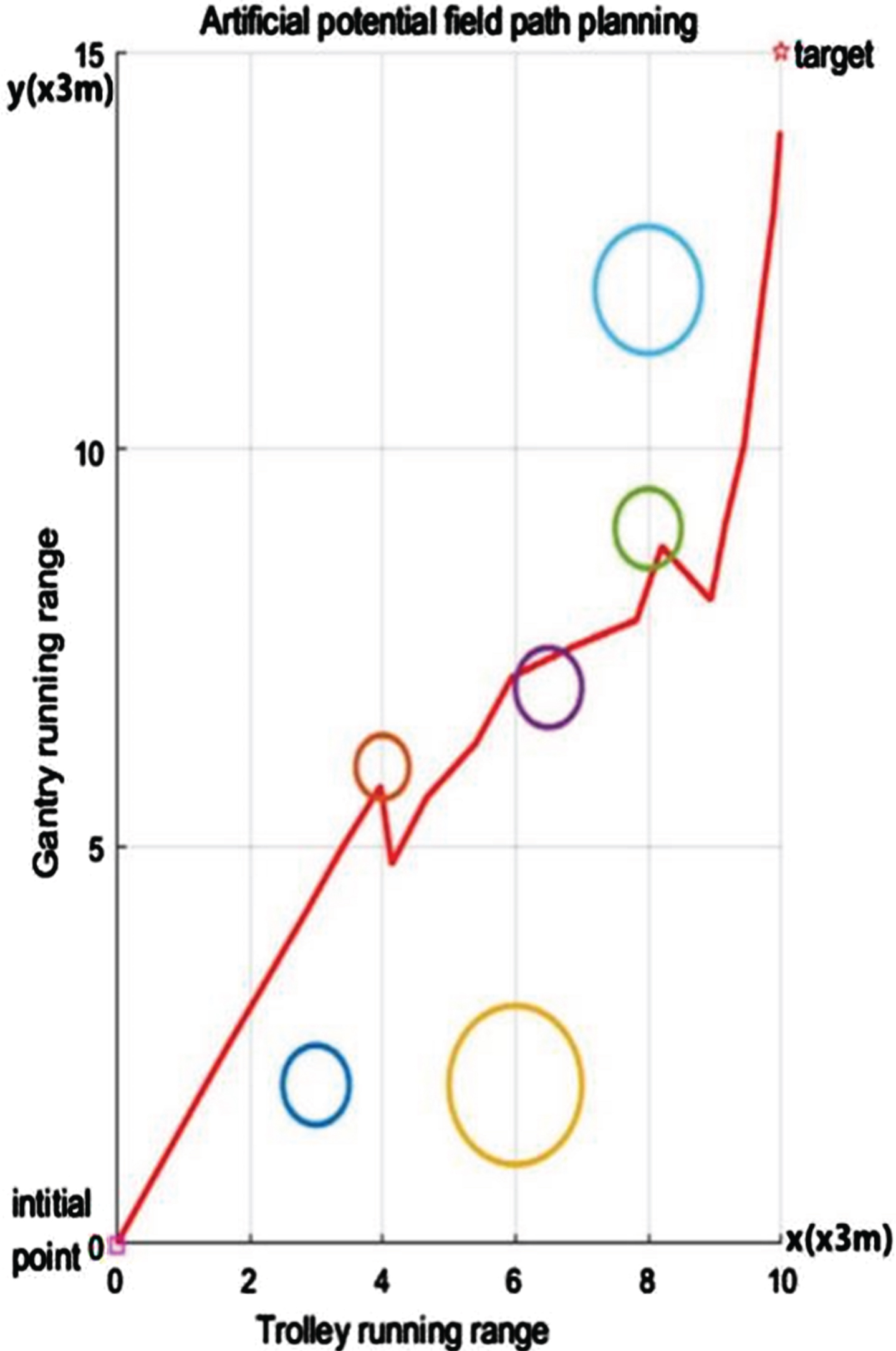
The second environment examined in this study was as follows: the starting point was (0, 0), the target point was (10, 15), the number of obstacles was 6, the central coordinates were (3, 2; 4, 6; 6, 2; 6.5, 7; 8, 9; 8, 12), the radii of the obstacle circles were 0.5, 0.4, 1, 0.5, 0.5, and 0.8, and the number of iterations was 200. The other parameter values were as follows: k = 5, η = 10, d₀ = 3, and l = 1.

As shown in Figs. 5 and 6, when the shape and size of the obstacle were not considered, the classical artificial potential field method could be used to plan a rough path, and the path trajectory did not pass through the points that represent the obstacles. However, if the outline of the obstacle is considered, as it was in this study, the path collides with the obstacle. There is no guarantee of the safety of the obstacles, and the path planning is a failure.

Fig.5

Path planning of the classical artificial potential field method in the first environment.

Fig.6

Path planning of the classical artificial potential field method in the second environment.

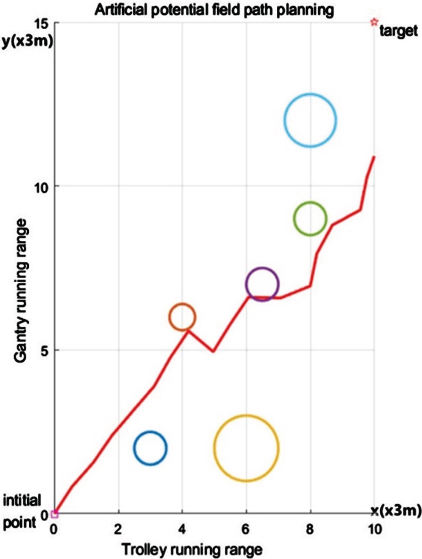
5.2 Simulation of double-layer artificial potential field method

In Figs. 7 and 8, the double-layer artificial potential field method was used for the path planning. Under normal circumstances, the path could avoid obstacles. However, if the repulsive forces of the potential field are superimposed, the path trajectory will be affected, and the path will collide with the edges of the obstacles.

Fig.7

Path planning of two-layer artificial potential field method in the first environment.

Fig.8

Path planning of the two-layer artificial potential field method in the second environment.

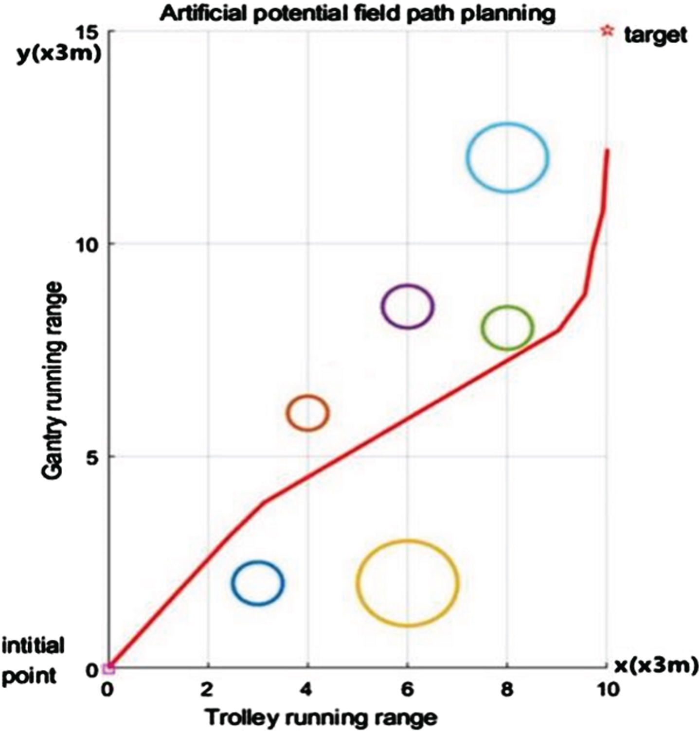
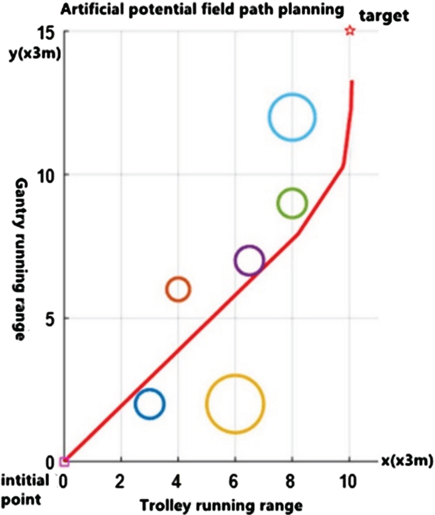
5.3 Simulation of fuzzy-double-layer artificial potential field method

Based on the double-layer artificial potential field method plus the path trajectory fuzzy processing method, the effect of the path planning is shown in Figs. 9 and 10. The simulation results were very good, and the path perfectly avoided all obstacles. Furthermore, the path lengths were shortened, and the lifting times were reduced.

Fig.9

Path planning of the fuzzy-double-layer artificial potential field method in the first environment.

Fig.10

Path planning of the fuzzy-double-layer artificial potential field method in the second environment.

6 Conclusion

In the case of ignoring the shape and size of the obstacle, the path planning simulation based on the classical artificial potential field method is a tortuous and rough broken line that does not pass the obstacle point, and requires many steps. When considering the contour of the obstacle, the path planning using the classical artificial potential field method cannot guarantee the safety of the obstacle, which is a kind of failed path planning.

In the simulation of path planning based on the double-layer potential field artificial potential field method, the phenomenon of hitting obstacles still appears, and this path planning requires more steps.

In this study, the classical artificial potential field method, double-layer artificial potential field method, and fuzzy-double-layer artificial potential field methods were simulated in two environments. Through comparison and analysis, it was concluded that the path planning based on the fuzzy-double-layer artificial potential field method could eliminate the problems of an unreachable target and local minima.

Footnotes

Acknowledgments

This achievement was funded by the graduate joint training base in Shanxi Province talent cultivation project funding (2018JD31).

References

Zhao

, The development trend of bridge crane at home and abroad and the idea of the product development of our factory, in: The Third Pan-Pearl River Delta Advanced Manufacturing Forum, Kunming, China, (2006), 48–51.

Tang

, Pan

, The application of intelligent control system on bridge crane, in: The 13th national automation application technology academic exchange meeting, Beijing, China, (2008), 1003–1036.

Zhang

, The intellectualization trend and development countermeasure of construction machinery, Technol Dev Enterp (4) (2012), 115–116.

Zhao

, Chen

, Research of path planning and obstacle avoidance mobile robot based on binocular vision, Eng Appl30(23) (2009), 5466–5470.

Jiang

, Wang

, Gong

J.W.

, Chen

H.Y.

, Research on Temporal Consistency and Robustness in Local Planning of Intelligent Vehicles, 41(3) (2015), 518–527.

Khatib

, Real-time obstacle avoidance for manipulators and mobile robots, in: 1985 IEEE International Conference on Robotics and Automation, St. Louis, Missouri, (1985), 500–505.

Xiu

, Chen

, A research on local path planning for autonomous vehicles based on improved APF method, 35 (2013), 808–811.

Zhang

, Lu

, Soccer robot path planning based on artificial potential field approach with simulated annealing, Mach Sci Technol (4) (2003), 547–548, 555.

, Sun

, Deng

, Algorithm based on massively parallel connectionist network for path planning, 36 (1996), 67–71.

10.

Song

, dissertation

Ph.D.

, School of information science and engineering, Shenyang University of Technology, Liaoning, China, 2017.

11.

Zhao

, Li

, Path planning for molile robot based on improved artificial potential field, Mach Design Manuf (7) (2017), 252–255.

12.

Liu

Z.Z.

, The Application of Artificial Potential Field in Intelligent Unmanned Vehicle Obstacle Avoidance System, Automation (2) (2013).

13.

Deng

, Wu

, Wang

, Mobile robot path planning with artificial potential field, Journal of University of Science and Technology Liaoning33(5) (2010), 460–463.

14.

, Zhang

, Ning

, Feng

, Li

, Path planning for Robot based on improved artificial potential field method, Eng Appl (24) (2013).

15.

Nara, Miyamoto, Takahashi, Position measurement of crane hook by vision and laser, IEEE Industrial Electronics6(10) (2006), 184–189.

16.

Yoshida

, Visual tracking and control of a moving overhead crance load, IEEE International Workshop on Advanced Motion Control (2006), 630–635.

17.

Lei Zhen, Lift path planning for a nonholonomic crawler crane, Automation in Construction31 (2013), 41–53.

18.

Panpan

, Parallel genetic algorithm based automatic path planning for crane lifting in complex environments, Automation in Construction62 (2016), 133–147.

19.

Lee

, Cho

, Ham

, et al., A BIM-and sensor-based tower crane navigation system for blind lifts, Automation in Construction (26) (2012), 1–10.

20.

Nagai

, Kaneshige

, Ueki

, Three-dimensional obstacle avoidance online path-planning method for autonomous mobile overhead crane, International Conference on Mechatronics & Automation, IEEE (2011), 1497–1502.

21.

Kawasaki

, Kaneshige

, Ueki

, Development of the autonomous mobile overhead traveling crane in consideration of on-line obstacle recognition, path planning and oscillating control, International Conference on Informatics in Control02 (2014), 382–389.