Real-time day ahead energy management for smart home using machine learning algorithm

Abstract

Smart grid is a sophisticated and smart electrical power transmission and distribution network, and it uses advanced information, interaction and control technologies to build up the economy, effectiveness, efficiency and grid security. The accuracy of day-to-day power consumption forecasting models has an important impact on several decisions making, such as fuel purchase scheduling, system security assessment, economic capacity generation scheduling and energy transaction planning. The techniques used for improving the load forecasting accuracy differ in the mathematical formulation as well as the features used in each formulation. Power utilization of the housing sector is an essential component of the overall electricity demand. An accurate forecast of energy consumption in the housing sector is quite relevant in this context. The recent adoption of smart meters makes it easier to access electricity readings at very precise resolutions; this source of available data can, therefore, be used to build predictive models., In this study, the authors have proposed Prophet Forecasting Model (PFM) for the application of forecasting day-ahead power consumption in association with the real-time power consumption time series dataset of a single house connected with smart grid near Paris, France. PFM is a special type of Generalized Additive Model. In this method, the time series power consumption dataset has three components, such as Trend, Seasonal and Holidays. Trend component was modelled by a saturating growth model and a piecewise linear model. Multi seasonal periods and Holidays were modelled with Fourier series. The Power consumption forecasting was done with Autoregressive Integrated Moving Average (ARIMA), Long Short Term Neural Memory Network (LSTM) and PFM. As per the comparison, the improved RMSE, MSE, MAE and RMSLE values of PFM were 0.2395, 0.0574, 0.1848 and 0.2395 respectively. From the comparison results of this study, the proposed method claims that the PFM is better than the other two models in prediction, and the LSTM is in the next position with less error.

Keywords

Energy management smart home energy forecast power management efficiency

1 Introduction

The present world is in an age of innovation and modernization. In this technologically emerging situation, things around us are getting smarter.

Smart meters allow more flexibility in demand-side management [1]. Every home has a smart meter in a traditional smart grid that links several smart appliances via a data network [2]. Electrical energy consumption forecasting plays a significant role in electricity production schedule as it specifies the amount of capital necessary for operating the power plants [3]. Accurate demand forecasting makes it possible to make the right decisions for future strategic planning. Various methods such as multiple regression, exponential smoothing, iterative reweighted least-squares, have been defined in the studies of Alfares and Nazeeruddin; Feinberg and Genethliou [4, 5].

The precise demand forecasts enables consumers to take part in demand response activities and obtains money from the service provider [6]. In response to the price with load signal forecast, consumers modify their energy usage timelines to minimize cost of electricity without affecting their level of comfort [7]. Using Demand-side management (DSM) [8], digital capability can be expanded with enhanced asset efficiency along with customer participation.

Makridakis et al. listed and analyzed many quantitative predicting techniques, including regressive analysis classical method of decomposition, Box and Jenkins [9] and smoothing methods.

Despite broad research, precise power consumption forecasting remains a challenge in smart grids. In study conducted by Taylor, these challenges were encountered by proposing Facebook PFM forecasting model that was introduced from Facebook in 2017 [10] by Sean J. Taylor and Ben Letham. For this work, the real-time power consumption dataset was used, and it represented power consumption per minute that was observed over nearly four years for a single house near Paris, France [11,42, 11,42].

In this paper, power consumption forecasting is estimated by three models namely, conventional state-space model ARIMA (Autoregressive Integrated Moving Average), nonlinear machine learning LSTM (Long Short Term Neural Memory Network) and the proposed PFM. The power consumption of four years (December 2006 to November 2010) real-time smart meter dataset of a single home near Paris is considered as a test system for the proposed method. The error metrics such as Mean Absolute Error (MAE), Root Mean Squared Logarithmic Error (RMSLE) and Root Mean Square Error (RMSE) and also Precision and F1 score were calculated and compared to prove the performance of the proposed PFM forecasting model. The test results showed the betterment of PFM that gives the forecast of power consumption very accurately comparing with Auto ARIMA and LSTM.

The rest of this paper is organized as follows. Section 2 elaborates the review of the literature. Section 3 explains descriptions of the power consumption dataset and conceptual method to model time series derivation, and it also describes the motivation of the present research work. Eventually, Section 4 deals with the simulation analysis and performance parameters of evaluation. Section 5 provides a comparative analysis of the research. Section 6 concludes and explores future work.

2 Literature survey

The electrical gadgets incorporate two-way communication capabilities for permitting the vitality administration framework to control the utilization [12]. Smart grid combines the use of sensors, networking, processing and control to improve the overall efficiency of the electrical power system [13]. Initiatives for smart grids are aimed at improving services, servicing and scheduling utilizing advanced technology to optimize power consumption and costs [14].

The conventional numerical time series replica was developed for forecasting load curve and peak demand in the study of Iglesias and Kastner [15].

Zhu et al. analyzed the problem of household energy consumption with the VAR construction model in China from 1980 to 2009 [16]. Kandananond et al. used various methods of prediction such as multiple linear regressions (MLR), artificial neural network (ANN) and autoregressive integrated moving average (ARIMA) to forecast energy consumption [17].

Li et al. calculated the total annual consumption with the transfer coefficient of the building using SVM [18]. Jain et al. reported results of energy modeling on multi-family housing in comparison with consumption of single-family homes aggregated at the construction stage [19]. In another study, the authors achieved promising results in resolving the inherent difficulties of researching individual household loads, a more difficult challenge than distributed loads [20]. Deep learning neural networks are commonly used in many fields, such as stock index forecasting [21, 22], solar irradiance prediction [23, 24], wind speed prediction [25,26, 25,26], etc. DLNN is introduced to more complex issues such as estimates of power consumption for individual households due to substantiate more internal hidden layers and algorithms related to classic ANNs [27].

Kong et al. [28] straightforwardly introduced a two-layer LSTM to the forecasting problems of single household power consumption. Samuel et al. [29] used Fourier analysis for identifying demand and solar production. The methods used for the time series approaches such as Kalman Filter Procedure, Box Jenkins approach, Regression approach and Spectral Expansion Methodology were carried out in the other studies [30, 31]. The author [32] used a Facebook PFM Sean algorithm, which was introduced by J. Taylor and Ben Letham from Facebook in 2017 to forecast the sales for the next year using sample sales data. Intelligent water droplets algorithm were introduced [40] for evaluating the problems in power system. Research challenges in Engineering field with the implementation solutions are discussed in [43].

Our literature survey concludes that the traditional prediction methods are subjective and the accuracy of the model chosen will depend on the forecaster’s ability and experience. The fundamental conceptual model and structural relations are not distinguished from some simple models of predictions. Linear seasonal model ARIMA needs to tune the non seasonal order argument (p, d, and q) and seasonal order arguments (P, D, Q, and s) and it takes time to tune the optimum parameters. The power consumption time series dataset is nonlinear and the forecasting need more accuracy.

In order to address these issues and to provide a practical “scale” prediction approach, a new Prophet Model is proposed. The proposed prophet model provides intuitive parameters which are easy to tune.

3 Motivation and methodology

Smart grid requires a day-ahead load forecasting of its customers for daily operations. In this paper, PFM is proposed as a procedure for the prediction of time series data based on an additive regression model in which non-linear trends fit.

3.1 Dataset and pre-processing

The time-series data set of individual household electricity consumption from the University of California, Irvine repository was considered in this proposed study.

3.2 Statistical normality test

The nonlinearity of the power consumption was checked by using the statistical histogram plot, Kurtosis and Skewness test [33]. Figure 1, shows that the ordered values are far away from the normal, so the power consumed by a single house is nonlinear.

Fig. 1

Probability plot of Global active power.

Furthermore, Kurtosis and Skewness of the power consumption dataset were measured to determine whether the power consumption data distribution was linear and normally distributed. Figure 2 shows that Kurtosis is greater than zero and skewness is greater than 1.

Fig. 2

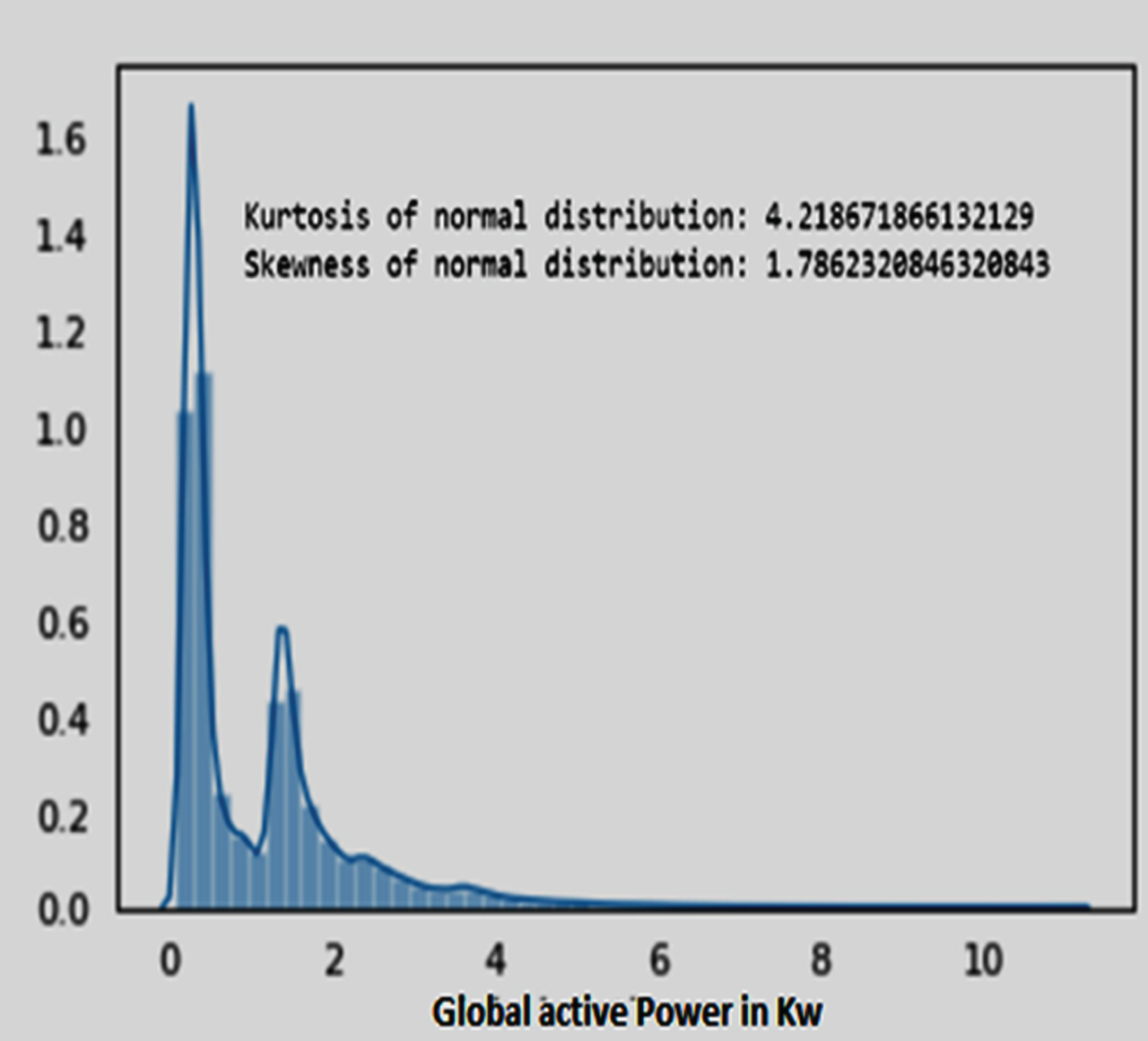
Kurtosis and Skewness of dataset.

3.3 Seasonal component test

Using the power consumption data, a plot was plotted between weekday and weekend power consumption. Figure 3 shows the plot between weekday and weekend power consumption, and it is understood that the power consumption differs in weekdays and weekends.

Fig. 3

Weekly and Weekend power consumption.

Figure 4 shows the box plot of yearly and quarterly power consumption. Figure 5 shows the graphical representation of residual, seasonal and trend components of the power consumption dataset.

Fig. 4

Yearly and quarterly power consumption throughout the year.

Fig. 5

Trend, seasonal, and residual components of dataset.

3.4 ARIMA model

ARIMA (Autoregressive Integrated Moving Average) is a machine learning regressive model category that captures in time series data a matching set of different standard temporal structures.

The model error is expressed by a moving average (MA (q)) component as a hybrid of former error terms e (t). The ARIMA model is given in Equation 1, $Yt = C + \sum_{i = 1}^{p} φ_{i} X_{t - i} + \sum_{i = 1}^{q} β_{i} ɛ_{t - 1} + ɛ_{t}$ (1)

Where,

Y_t- Predicted term at t of time series Y

c - Constant

X_t-i - lag of the series

ɛ_t-i - Error at t-i lag

φ, β - Coefficient of the lag

t – Time

3.5 LSTM (Long Short Term Neural Memory Network) model

The LSTM was suggested by Hochreiter and Schmidhuber as a special cyclic neural network [33, 41]. The intrinsic relationships were extracted by the cyclic interaction between neurons and the time-series data were modeled [34 , 36]. The LSTM network’s memory cell structure is shown in Fig. 6.

Fig. 6

LSTM structure.

The memory module has input gate, forgetting gate, output gate and one loop connecting unit. LSTM also can handle huge information.

3.6 Proposed PFM

The authors have proposed PFM for the application of power consumption forecasting. The Proposed PFM uses three major mechanisms of a decomposable time series: trend, seasonality and holidays. $y (t) = g (t) + s (t) + h (t) + ɛ (t)$ (2)

y(t): Predicted term at time t, g(t): Linear or logistic growth curve piece by piece to model non-periodic time-series changes, s(t): Periodic variation (e.g. weekly/yearly seasonality), h(t): Holidays effect (user-provided) with uneven plant, ɛ(t): Error term refers to any uncommon changes that the model does not accommodate.

In order to fit the historical data, the model must be able to incorporate trend changes. So, the change points at which the rate of growth is allowed are described explicitly. The rate at any time is defined as $k + a (t)^{τ} δ_{j}$ (3)

Where, $a (t) = {\begin{matrix} 1 {if t ⩾ s_{j} \end{matrix} 0 otherwise$

S – Change points at time s_j, j = 1, 2, … . S

δ_j – Rate change occurs at time s_j

The adjustment at change point j is $γ_{i} = (S_{j} - m - \sum_{t < j} γ_{t}) (1 - \frac{k + \sum_{t < t} δ_{t}}{k + \sum_{t ⩽ t} δ_{t}})$ (4)

The trend component is modelled as $g (t) = (k + a (t)^{τ} δ) t + (m + a (t)^{τ} γ)$ (5)

Where, k – growth rate

M – Offset parameter

γ_i settos_iδ_j to make continuous function

δ_j ∼ Laplace (0, τ)

τ – controls the flexibility of the model

PFM introduces the predictive problem as a curve-fitting exercise rather than looking specifically at each observation’s time-based dependence in a time series. The following function approximates the s(t) seasonal effects by the following Fourier series: $s (t) = \sum_{n = 1}^{N} a_{n} (a_{n} cos (\frac{2 π nt}{P}) + b_{n} sin (\frac{2 π nt}{P}))$ (6)

P is the period. For fitting seasonality, it is necessitated to find the 2 N parameters β = [a₁, b₁ . . . . . . . , a_N,b_N] ^τ. This is achieved by creating a seasonality vector matrix for each value of our historical and future data, e.g. with weekly seasonality and N = 3, $x (t) = [cos \frac{2 π (3) t}{7}, . . . . . . sin (\frac{2 π (3) t}{7}]$ (7)

Then the seasonal component is s (t) = x (t) β, β ∼ Normal (0, σ²). Shortening the series at N introduces a low-pass filter to the seasonality, which allows the N to counterpart seasonal trends that shift faster, although with increased risk of over fitting. N = 10 for yearly seasonality and N = 3 for weekly seasonality.

An indicator function is added to represent whether time t is during holiday ‘i’ and the parameter Ki, which means the corresponding change in forecast is assigned for each holiday. This is achieved like seasonality by creating a regressor matrix. $Z (t) = [1 (t \in D_{1}), . . . . 1 (t \in D_{2})]$ (8) $h (t) = Z (t) k, k \sim Normal (0, v^{2})$ (9) $y (m, δ, β, κ, \in) \sim N (g (t) + s (t) + h (t), \in)$ (10)

Figure 7 shows the structure of the PFM. Time series data have the trend, seasonal and holiday’s components. These models are combined as a PFM represented in the Equation (10). The parameters τ and sigma control the regularization on the model seasonality.

Fig. 7

Structure of PFM.

4 Simulation study

As per the explanation given in section 4, the models were implemented in Anaconda 3 open source software, and the performance parameters were measured.

Figure 8 shows the steps involved in the present work.

Fig. 8

Flowchart of power forecasting process.

4.1 Performance criteria

Proposed PFM’s predictive results were compared with existing modern methods, including ARIMA model and LSTM. Four error metrics were calculated, including Root-Mean-Square Error (RMSE), Mean Absolute Error (MAE) and Root Mean Squared Logarithmic Error (RMSLE Equations (11–17) list the formulations of the above metrics. $MSE = \frac{1}{N} \sum_{i = 0}^{N} {(y_{i} - {\hat{y}}_{i})}^{2}$ (11) $RMSE = \sqrt{\frac{1}{N} \sum_{i = 0}^{N} {(y_{i} - {\hat{y}}_{i})}^{2}}$ (12) $MAE = \frac{1}{N} | y_{i} - {\hat{y}}_{i} |$ (13) $RMSLE = \log (p_{i} + 1) log ai + 1$ (14)

where y_i is an actual testing sample value $\hat{y_{i}} is the forecast result of y_{i}$ (15) $\hat{y} is them ean of predicted$ (16)

N is the total number of samples tested.

Precision and F1 score also measured to compare the performance. It is measured by, $Precision = \frac{TruePositives}{True Positives + False Positives}$ (17)

Recall means the percentage of total significant results that are correctly forecasted. $Recall = \frac{Truepositive}{TruePositive + FalseNegatives}$ (18) $F 1 = 2 \times \frac{Pr ecision \times Re call}{Pr ecision + Re call}$ (19)

Time taken for tuning the optimum values for the seasonal parameters (P, D, Q, m) and non-seasonal parameters (p, d, q) of ARIMA model was noted.

4.2 ARIMA model simulation

The ARIMA model needs the tuning parameters, non-seasonal and seasonal order arguments. Using a standardized procedure the ARIMA seasonal model is implemented to forecast power consumption.

Figure 9. shows the plot of actual global active power consumption in kilowatts and forecasted global active power consumption plot from June 2009 to December 2009. This plot shows that the ARIMA model forecasting has the deviation from the actual global active power consumption in kilowatts. Table 1 gives the evaluation parameters of the ARIMA forecasting model. The model has 80% as F1 score and 76% as precision. The time taken for tuning the optimum value for seasonal and non-seasonal parameters of ARIMA model was 1452.39 sec.

Fig. 9

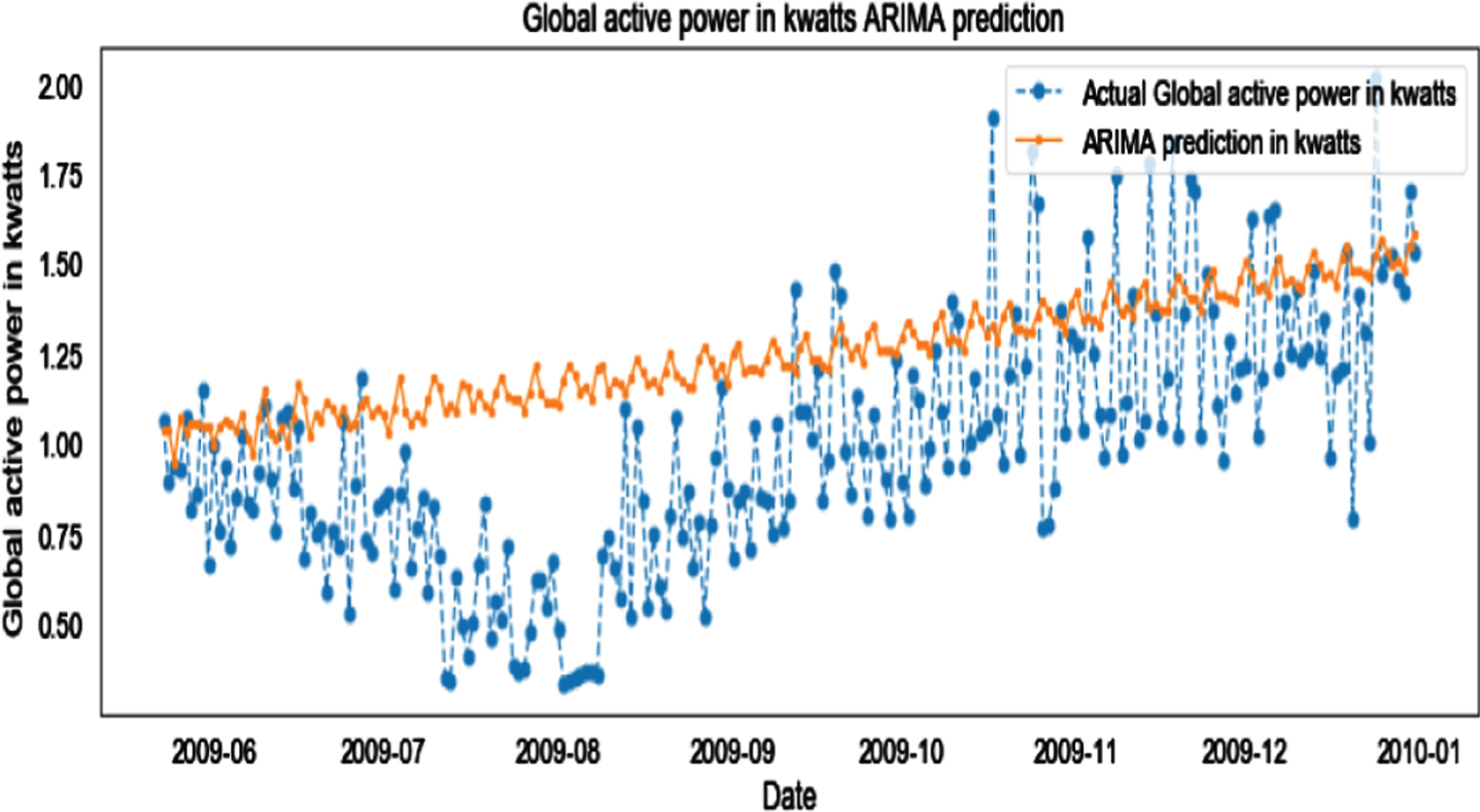
ARIMA forecasting model with Test set.

Table 1

ARIMA performance evaluation

RMSE	MSE	MAE	RMSLE	Precision	F1 score	Tuning time	Training time
0.3833	0.1469	0.3216	0.1994	76%	80%	1452.39 sec	56.3 sec

The fitness of the model is analyzed by plotting the diagnostic plot. Figure 10 shows the diagnostic plot of the ARIMA model, which was drawn from the residual error of forecasting power consumption. From this Fig. 10, it is observed that the residuals are not dispersed normally.

Fig. 10

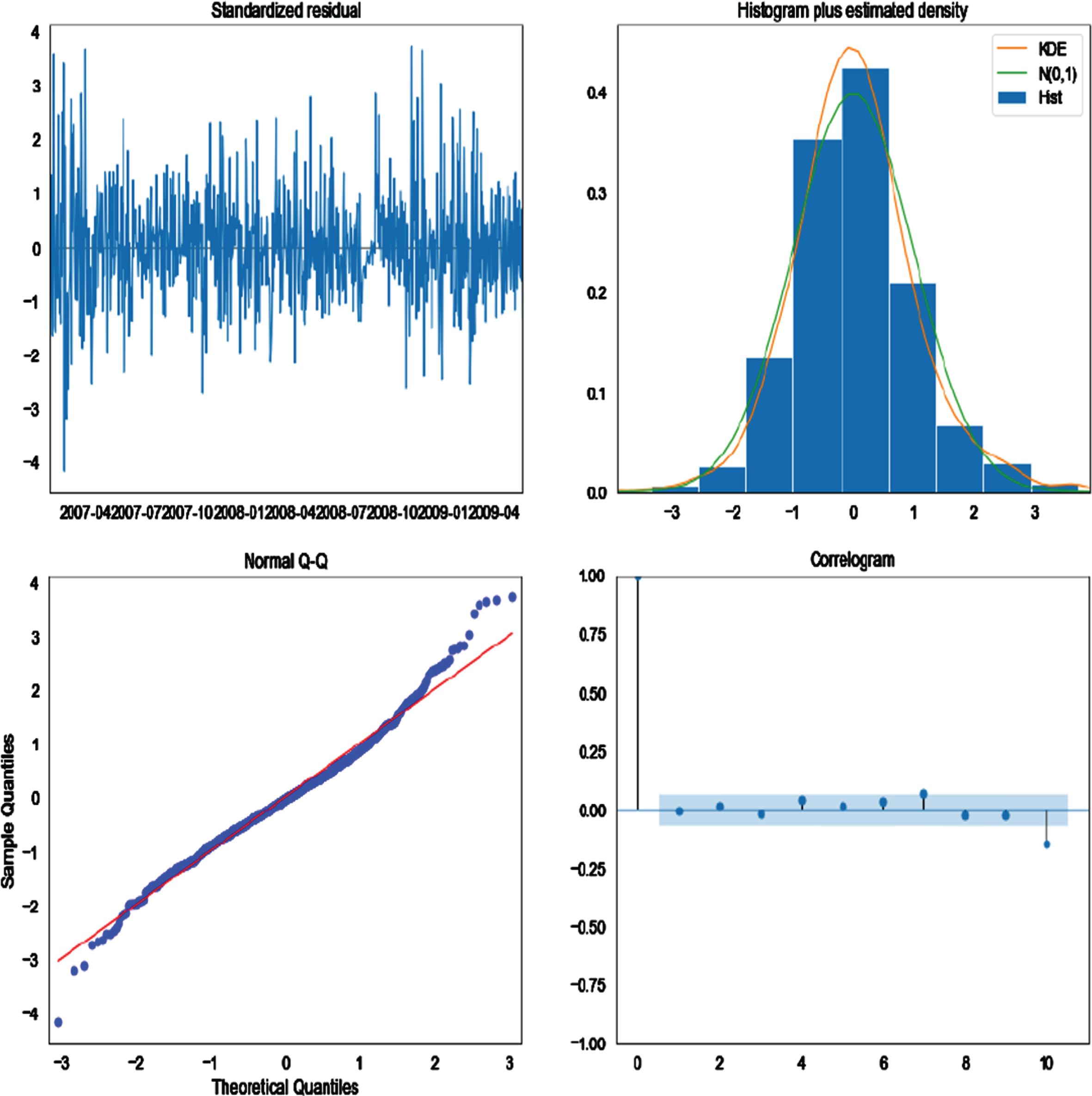
Diagnostic plot of ARIMA model.

These observations result that the trained ARIMA model cannot provide a satisfactory forecast for the power consumption dataset.

4.3 LSTM model simulation

To overcome the problems in ARIMA, the supervised LSTM model was implemented.

Figure 11 shows the plot between actual and forecasted Global active power consumption in kilowatts.

Fig. 11

LSTM power consumption Forecasting.

Table 2 gives the evaluation parameters of the LSTM forecasting model. Even though RMSE, MSE, MAE and RMSLE parameters are better than ARIMA model, the precision is decreased to 72%, and the F1 score is decreased to 77%. Time taken to train the LSTM model with optimum setting was 7.59 sec.

Table 2

LSTM performance evaluation

RMSE	MSE	MAE	RMSLE	Precision	F1 score	Training Time
0.2826	0.0799	0.2290	0.1440	72%	77%	7.6 sec

Figure 12 shows the LSTM diagnostic plot during training and testing.

Fig. 12

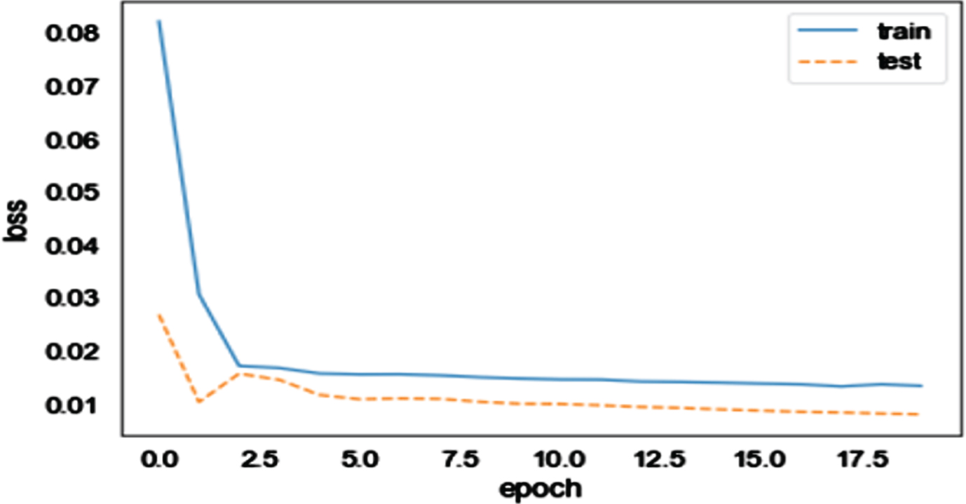
LSTM diagnostic plots.

4.4 PFM simulation

To overcome the problems in ARIMA and LSTM models, a new PFM has been proposed. The dataset should be converted into two columns.

From Fig. 13, it is inferred that the model follows the actual pattern. So, during the training, it followed the seasonality effect in the historical power consumption dataset.

Fig. 13

PFM power consumption forecasting.

From Fig. 14, it is understood that the proposed model identifies that the key trend in the power consumption dataset is better than ARIMA and LSTM.

Fig. 14

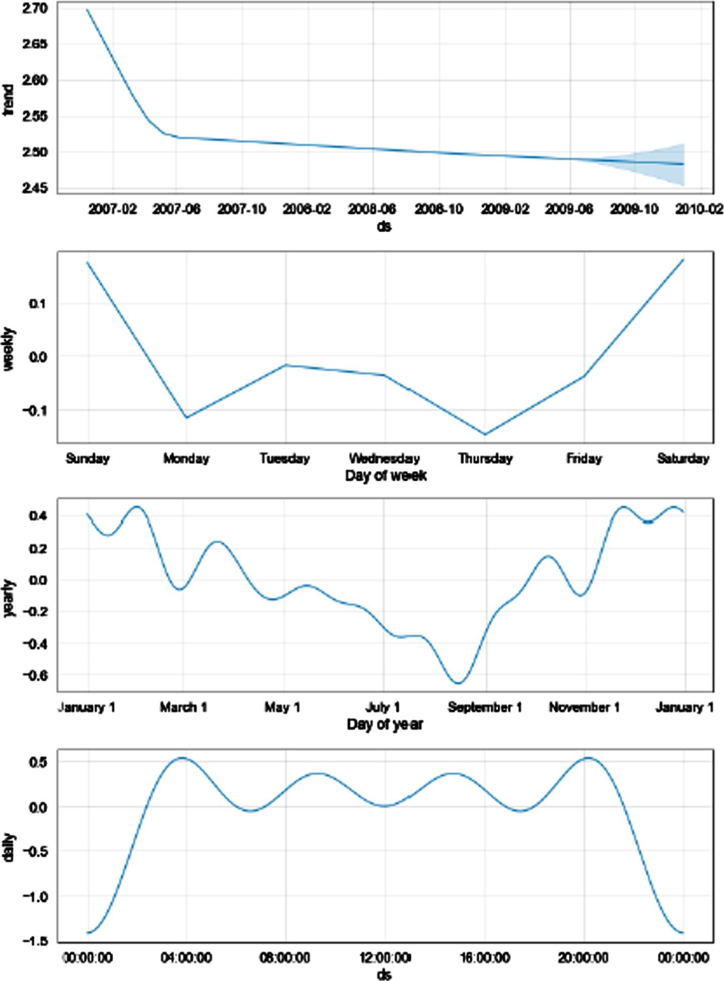
Components of PFM.

Table 3 shows that the improved RMSE, MSE, MAE and RMSLE values were 0.2395, 0.0574, 0.1848 and 0.2395, respectively. The precision and F1 score were also improved as 80% and 81%, respectively. The proposed model automatically traces the trend and seasonality effect of the power consumption from the date columns. Time taken by the proposed model to train was 4.403 sec.

Table 3

PFM performance evaluation

RMSE	MSE	MAE	RMSLE	Precision	F1 score	Training time
0.2395	0.0574	0.1848	0.1226	80%	81%	4.4 sec

5 Comparative analysis

This section provides a comparison between the performance evaluation parameters of the three implemented forecast models.

5.1 Comparison based on performance metric measure

Table 4 shows that ARIMA model has the highest RMSE value 0.3823, and the proposed PFM has the minimum value 0.2395. So, the lowest value of RMSE results in highest accuracy in forecasting. So, based on RMSE, the proposed model has the highest accuracy.ARIMA model has the highest MSE value 0.1469, and the proposed PFM has the minimum value 0.0574. So, the lowest value of MSE results in highest accuracy in forecasting. So, based on MSE, the proposed model has the highest accuracy. From Table 4 ARIMA model has highest value |MAE 0.3216 and the proposed PFM has the minimum value 0.1848. The lowest value of MSE results highest accuracy in forecasting. So, based on MAE the proposed model has the highest accuracy.

Table 4
RMSE

MODELS/PARAMETER ARIMA LSTM PFM

RMSE 0.3823 0.2826 0.2395

MSE 0.1469 0.0799 0.0574

MAE 0.3216 0.2290 0.1848

RMSLE 0.1994 0.1440 0.1226

MODELS/PARAMETER	ARIMA	LSTM	PFM
RMSE	0.3823	0.2826	0.2395
MSE	0.1469	0.0799	0.0574
MAE	0.3216	0.2290	0.1848
RMSLE	0.1994	0.1440	0.1226

5.2 Precision and F1 score

Table 8 lists the Precision and F1 score of the ARIMA, LSTM and PFM modes, and Fig. 15 displays the comparison bar chart.

Fig. 15

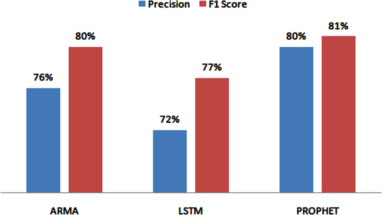
Precision and F1 score.

Table 5 illustrates that the proposed PFM forecast model has improved precision, and F1 score is 80% and 81 % respectively, which is higher than the other two models.

Table 5

Precision and F1 score

Model	ARMA	LSTM	PFM
Precision	76%	72%	80%
F1 Score	80%	77%	81%

5.3 Based on Daily, Weekly, Monthly and quarterly forecasting

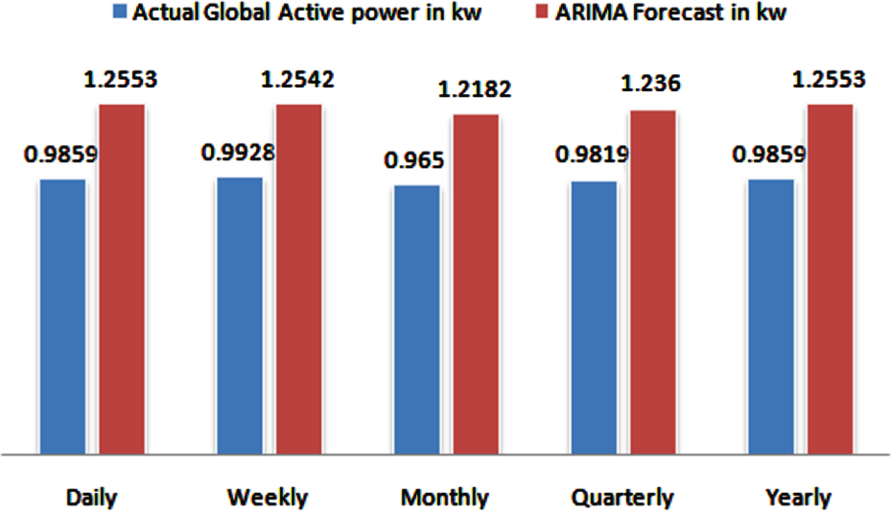
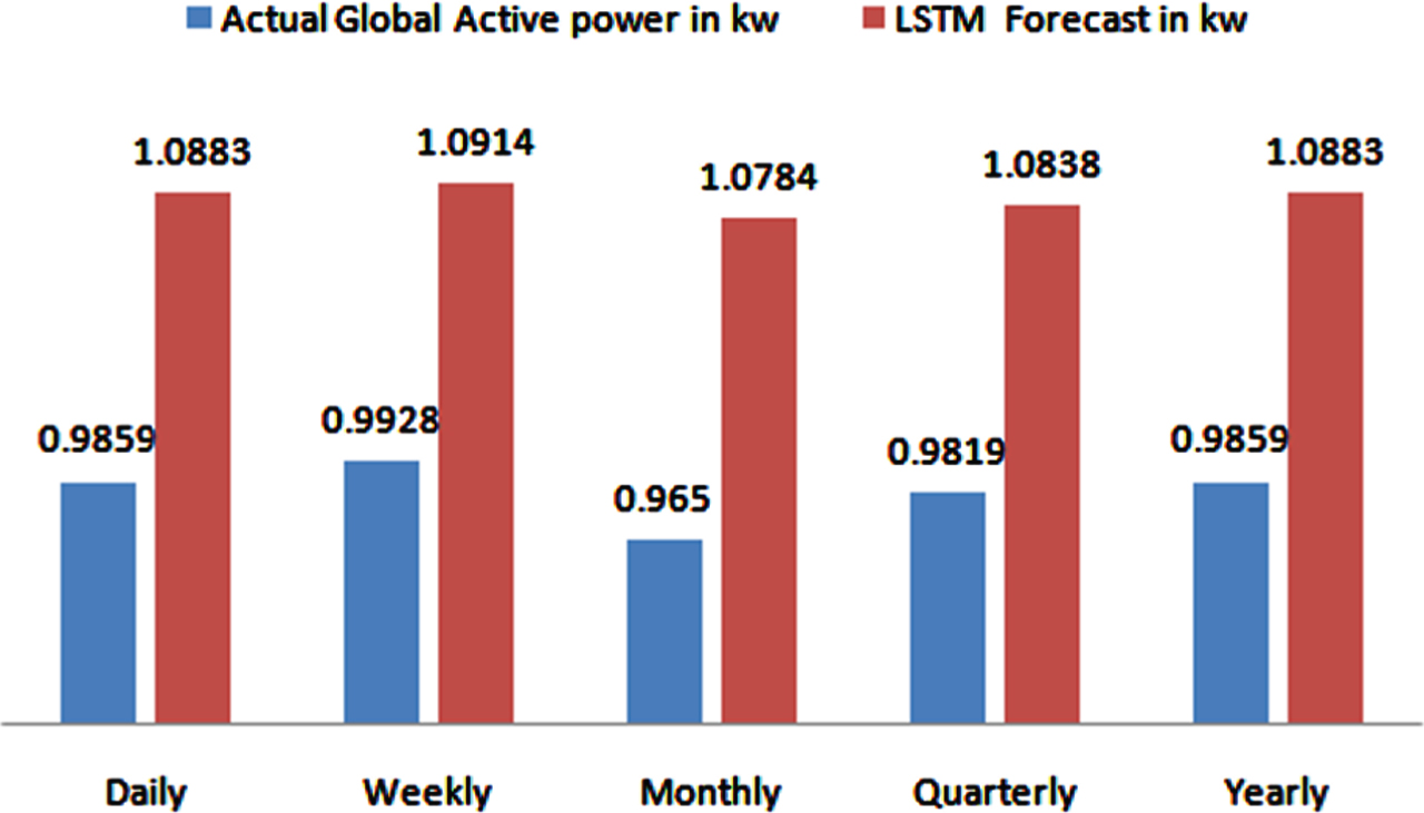
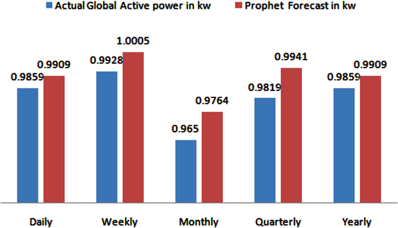
Table 6 displays the mean value of actual and forecasted values of ARIMA, LSTM and PFM based on daily, weekly, monthly and quarterly.

Table 6
Forecasting performance

Seasonal Global Active power in kilowatts

Actual ARIMA LSTM PFM

Forecast Error Forecast Error Forecast Error

Daily 0.9859 1.2553 0.2694 1.0883 0.1024 0.9909 0.005

Weekly 0.9928 1.2542 0.2614 1.0914 0.0986 1.0005 0.0077

Monthly 0.965 1.2182 0.2532 1.0784 0.1134 0.9764 0.0114

Quarterly 0.9819 1.236 0.2541 1.0838 0.1019 0.9941 0.0122

Yearly 0.9859 1.2553 0.2694 1.0883 0.1024 0.9909 0.005

Seasonal	Global Active power in kilowatts
Daily	0.9859	1.2553	0.2694	1.0883	0.1024	0.9909	0.005
Weekly	0.9928	1.2542	0.2614	1.0914	0.0986	1.0005	0.0077
Monthly	0.965	1.2182	0.2532	1.0784	0.1134	0.9764	0.0114
Quarterly	0.9819	1.236	0.2541	1.0838	0.1019	0.9941	0.0122
Yearly	0.9859	1.2553	0.2694	1.0883	0.1024	0.9909	0.005

ARIMA model has seasonal parameters P, D, Q, s and it is tuned to the optimum values For tuning, the time taken by the ARIMA model was 1452.39 sec. However, Table 9 shows that when compared to ARIMA, the forecasted error is improved. While finding the relationships between ARIMA and LSTM, the proposed PFM shows the less forecasted error since it can trace the trend and seasonality

From Fig. 16 it is understood that the ARIMA model does not follow the seasonality, and it predicts based on the trend component.

Fig. 16

ARIMA power consumption forecasting.

From Fig. 17 it can be understood that the LSTM model forecasts the power consumption closer than ARIMA. But LSTM does not forecast much closer. Since LSTM trained with the past values and did not train with the seasonality, i.e., weekend consumption was larger than the weekday’s consumption. This seasonality effect is not followed by the LSTM. Even though it had the lowest performance error, the actual value predicted was less compared to the actual value.

Fig. 17

LSTM power consumption forecasting.

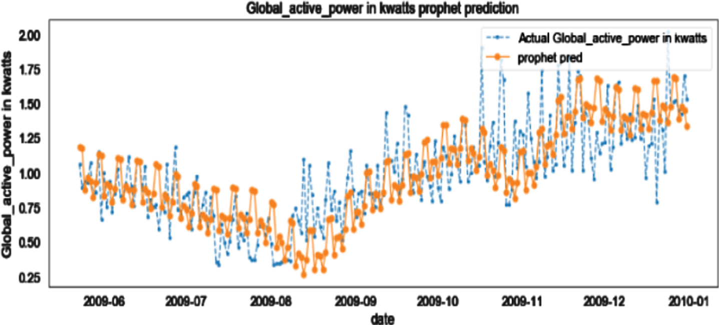
From Fig. 18 it is understood that the PFM follows the seasonality, and it predicts based on this. So, the forecasted power consumption is closer with the actual global active power.

Fig. 18

PFM Power Forecasting.

The periods for training ARIMA, LSTM and the proposed PFM are showed in Table 7. According to Table 10, ARIMA model was taken 1452.39 sec for tuning optimum parameters value of seasonal (P, D, Q, s) and non-seasonal (p, d, q) orders and 56.34 sec for training. Training time needed for LSTM model was 7.6 sec. But the proposed model’s training time was only 4.4 sec, which is the minimum time when compared to the time required by ARIMA and LSTM.

Table 7

Training time of ARIMA, LSTM and PFM

Model	ARIMA	LSTM	PFM
Training Time	56.3 sec	7.6 sec	4.4 sec

Figure 19 indicates that the PFM forecast follows the actual power consumption much closer.

Fig. 19

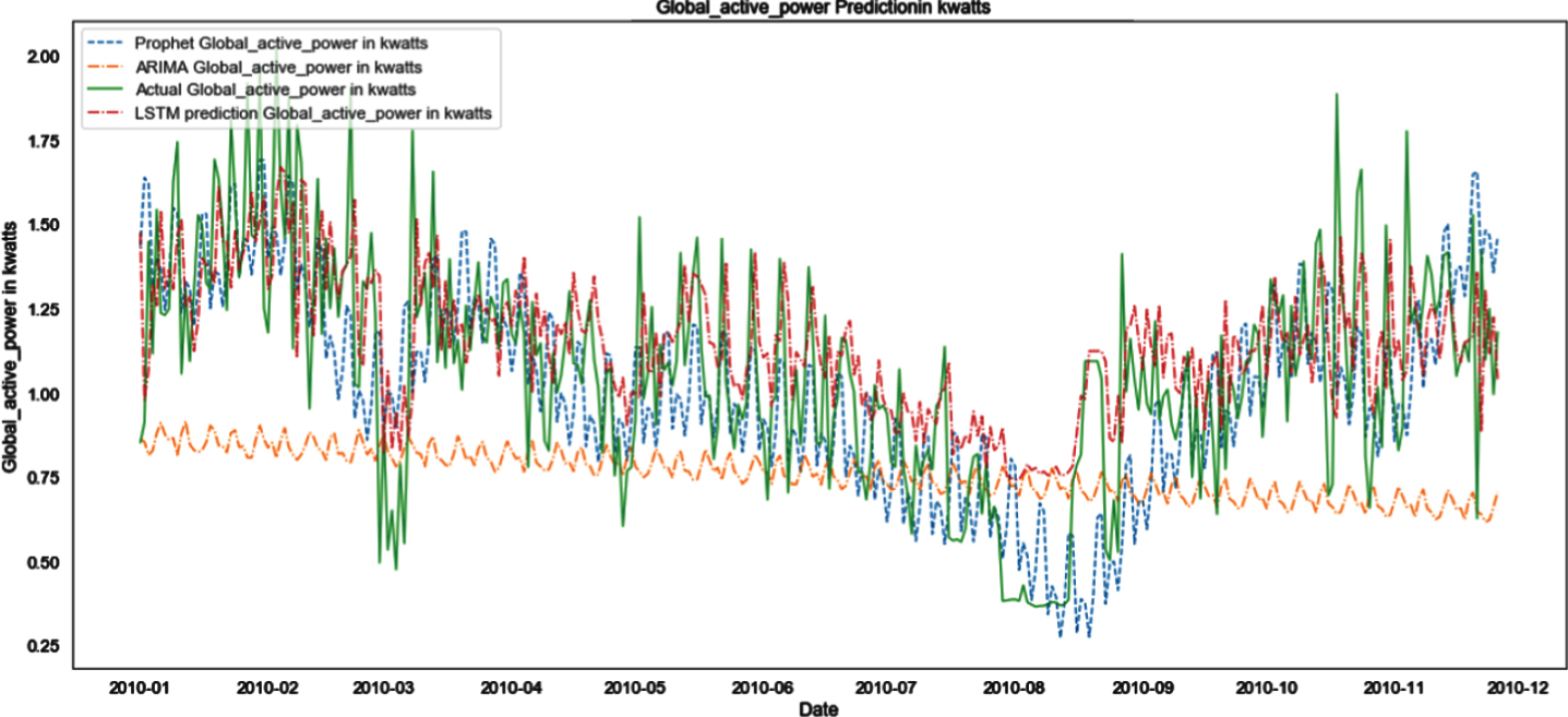
ARIMA, LSTM, PFM with Global Active Power in K watts.

In this proposed method, the three dissimilar models (ARIMA, LSTM and PFMs) are examined for day a-head power consumption of a residence. The ARIMA and LSTM achieved poor performance when compared to PFM forecasting model [37, 38].

6 Conclusion

To forecast power consumption, initially ARIMA model was implemented. The model took 1452.9 sec for setting the parameter and 56.34 sec for training. Precision was 80% but the value of F1 score as 76% and RMSE value as 0.383 were not satisfied. After this LSTM was implemented which took 7.6 sec for training and improved RMSE value as 0.2826 and the F1 score as 77% but the precision was decreased to 72%. Then, Prophet Model was applied for forecasting power and implemented PFM.

The PFM improved the Precision and F1 score as 80% and 81% respectively and also it improved the RMSE value as 0.2395. The training time also reduced as 4.403 sec. According to these comparisons we claim that our proposed PFM performs better than ARIMA and LSTM for forecasting power consumption of a house.

The outcome shows that the proposed PFM forecast model outperforms all other models. According to the error metrics, it gives the lowest RMSE, MSE, MAE and RMLSE. And also, the proposed PFM has better precision and F1 score when compared to the ARIMA and LSTM models. The time needed for training the proposed model is also minimum when compared to ARIMA and LSTM models. The results of the comparison show that the model of PFM prediction outlines the best alternative methods tested with high certainty.

In the future work, this PFM can be applied to the forecasting of single home appliances operating period without compromising their sophistication. As continued research, the authors propose the use of other uncontrollable variables in our systems, such as temperature or direct solar irradiation, effects of local stationary or mobile batteries to enhance the accuracy of forecasts.

References

Elma

, Gabbar

H.A.

, Perspectives of Demand-Side Management Under Smart Grid Concept. Energy Conservation in Residential, Commercial and Industrial Facilities (2018), 225–248. doi: 10.1002/9781119422099.ch7

Ur Rehman

, Fatima

, Khan

, Shah

, Wasim Ahmad

, Din

and Rehman

, Energy optimization in a smart community grid system using genetic algorithm, International Journal of Communication Systems (2019), e4265. doi: 10.1002/dac.4265

Zhu

, Wang

, Zhao

, Wang

, A seasonal hybrid procedure for electricity demand forecasting in China, Applied Energy88(11) (2011), 3807–3815. doi: 10.1016/j.apenergy.2011.05.005

Alfares

K.H.

, Nazeeruddin

, Electric load forecasting: literature survey and classification of methods, International Journal of Systems Science33(1) (2002), 23e34. ISSN 1464-5319.

Feinberg

E.A.

, Genethliou

, Load forecasting, applied mathematics for restructured electric power systems, Springer Link2005, 269e85. doi: 10.1007/0-387-23471-3_12

Park

, Ryu

, Choi

, Kim

, Data-driven baseline estimation of residential buildings for demand response, Energies8 (2015), 10239–10259.

Vardakas

J.S.

, Zorba

, Verikoukis

C.V.

, A Survey on Demand Response Programs in Smart Grids: Pricing Methods and Optimization Algorithms, IEEE Commun Surv Tutor17 (2015), 152–178.

Bruce

, Bowerman

, Connell

T.O’.

, Koehler

A.B.

, Forecasting, time series, and regression: an applied approach, 4th ed. The United States of America: Thomson Brooks (2005).

Makridakis

, Wheelwright

S.C.

, Hyndman

R.J.

, Forecasting: Methods and Applications, 3 ed. Wiley, Inc.,New York, (1998).

10.

Taylor

S.J.

, Letham

, Forecasting at scale, Peer J Preprints5 (2017), e3190v2 https://doi.org/10.7287/peerj.preprints.3190v2.

11.

UCI repository of machine learning database [Online]. Available: https://www.kaggle.com/uciml/electric-power-consumption-data-set.

12.

Arghira

, Hawarah

, Ploix

, Jacomino

, Prediction of appliances energy use in smart homes, Energy48(1) (2012), 128–134.

13.

Gellings Clark

, The smart grid: enabling energy efficiency and demand response, (2009), ISBN 0-88173-624-4, USA;

14.

Ipakchi

, Albuyeh

, Grid of the future, IEEE Power and Energy Magazine, Digital Object Identifier8(3) (2009), 20e9. 10.1109/MPE.2008.931384, ISSN 1540-7977

15.

Iglesias

, Kastner

, Analysis of similarity measures in times series clustering for the discovery of building energy patterns, Energies6 (2013), 579–597.

16.

Zhu

, Guo

, Feng

, Household energy consumption in China: Forecasting with BVAR model up to 2015, In 2012 Fifth International Joint Conference on Computational Sciences and Optimization (2012), 654–659. IEEE.

17.

Kandananond

, Forecasting Electricity Demand in Thailand with an Artificial Neural Network Approach, Energies4 (2011), 1246–1257.

18.

, Ren

, Meng

, Prediction Model of Annual Energy Consumption of Residential Buildings, In Proceedings of the 2010 International Conference on Advances in Energy Engineering, Beijing, China, (2010), 223–226.

19.

Jain

R.K.

, Smith

K.M.

, Culligan

P.J.

, Taylor

J.E.

, Forecasting energy consumption of multi-family residential buildings using support vector regression: Investigating the impact of temporal and spatial monitoring granularity on performance accuracy, Applied Energy123 (2014), 168–178.

20.

Armano

, Marchesi

, Murru

, A hybrid genetic-neural architecture for stock indexes forecasting, Inform Sci170 (2005), 3–33.

21.

Yildiz

, Bilbao

, Dore

, Sproul

, Recent advances in the analysis of residential electricity consumption and applications of smart meter data, Applied Energy208 (2017), 402–427.

22.

Rather

A.M.

, Agarwal

, Sastry

, Recurrent neural network and a hybrid model for prediction of stock returns, Expert Syst Appl42 (2015), 3234–3241.

23.

Wang

, Wang

, Li

, Peng

, Liu

, Deep belief network based deterministic and probabilistic wind speed forecasting approach, Appl Energy182 (2016), 80–93.

24.

Alzahrani

, Shamsi

, Dagli

, Ferdowsi

, Solar irradiance forecasting using deep neural networks, Procedia Comput Sci114 (2017), 304–313.

25.

Almalaq

, Edwards

, A Review of deep learning methods applied on load forecasting, In Proceedings of the 2017 16th IEEE International Conference on Machine Learning and Applications (ICMLA), Cancun, Mexico, 18–21 (2017), 511–516.

26.

Khodayar

, Kaynak

, Khodayar

M.E.

, Rough deep neural architecture for short-term wind speed forecasting, IEEE Trans Ind Inf13 (2017), 2770–2779.

27.

Voyant

, Notton

, Kalogirou

, Nivet

M.L.

, Paoli

, Motte

, Fouilloy

, Machine learning methods for solar radiation forecasting: A review, Renew Energy105 (2017), 569–582.

28.

Kong

, Dong

Z.Y.

, Jia

, Hill

D.J.

, Xu

, Zhang

, Short-term residential load forecasting based on LSTM recurrent neural network, IEEE Trans Smart Grid (2017).

29.

Samuel Matthew

, Dumlao

and Ishihara

, Reproducing solar curtailment with Fourier analysis using Japan dataset, Energy Reports6 Supplement 2 (2020), 199–205. https://doi.org/10.1016/j.egyr.2019.11.063.

30.

Mahalanabis

A.K.

, Kothari

D.P.

, Ahson

S.I.

, Computer Aided Power System Analysis and Control; Tata McGraw-Hill Publishing Company limited: New Delhi, India, (1988).

31.

Box

G.E.

, Jenkins

G.M.

, Time Series Analysis Forecasting and Control, Holden-Day: San Fransisco, CA, USA, (1976).

32.

https://help.gooddata.com/doc/en/reporting-and-dashboards/maql-analytical-query-language/maql-expression-reference/aggregation-functions/statistical-functions/predictive-statistical-use-cases/normality-testing-skewness-and-kurtosis.

33.

Hochreiter

, Schmidhuber

, Long short-term memory, Neural Computation9 (1997), 1735–1780. https://doi.org/10.1162/neco.1997.9.8.1735.

34.

Gao

, Location prediction algorithm of moving object based on LSTM, Computer Science and Exploration13 (2019), 23–34. https://doi.org/10.3778/j.issn.1673-9418.1801029.

35.

Kovárík

, Klímek

, The usage of time series control charts for financial process analysis, Journal of Competitiveness4(3) (2012), 29–45. doi: 10.7441/joc.2012.03.03

36.

Chukurna

, Nitsenko

, Kralia

, Sahachko

, Morkunas

, Volkov

, Modelling and managing the effect of transferring the dynamics of exchange rates on prices of machine-building enterprises in Ukraine, Polish Journal of Management Studies19(1) (2019), 117–129.

37.

Dvořáček

, Sousedíková

, Krzemień

and Sánchez

A.S.

, Focus on some aspects of market price trends for tungsten, Acta Montanistica Slovaca22(2) (2017), 126–135.

38.

Bilan

, Strielkowski

, Karbach

, Mentel

, Secure development of country and competitiveness issues: Case of Germany’s energy security, Journal of Security and Sustainability Issues6(3) (2017), 329–342. doi: 10.9770/jssi.2017.6.3(1)

39.

Hussain

H.I.

, Slusarczyk

, Kamarudin

, Thaker

H.M.T.

, Szczepańska

, - Woszczyna, An investigation of an adaptive neuro-fuzzy inference system to predict the relationship among energy intensity, globalization, and financial development in major ASEAN economies, Energies13(4) (2020), art. no. 850. doi: 10.3390/en13040850

40.

Sheela

, Sowmya

, Gowri Shankar

, Optimal placement and sizing of renewable energy generation considering uncertainities using intelligent water drops algorithm, International conference on Innovations in Information, Embedded and Communication Systems,Volume III, (2017).

41.

Lazib

, Zhao

, Qin

, Liu

, Negation scope detection with recurrent neural networks models in review texts, International Journal of High Performance Computing and Networking13(2), 211–221.

42.

Gupta

, Agrawal

D.P.

, Yamaguchi

, Handbook of Research on Modern Cryptographic Solutions for Computer and Cyber Security Malicious web pages detection using feature selection techniques and machine learning, International Journal of High Performance Computing and Networking14(4), 473–488.

43.

Veluru

, Gupta

B.B.

, Privacy preserving text analytics: research challenges and strategies in name analysis, In Standards and standardization: concepts, methodologies, tools, and applications (pp. 1415–1435). IGI Global.

Seasonal	Global Active power in kilowatts
	Actual	ARIMA		LSTM		PFM
		Forecast	Error	Forecast	Error	Forecast	Error
Daily	0.9859	1.2553	0.2694	1.0883	0.1024	0.9909	0.005
Weekly	0.9928	1.2542	0.2614	1.0914	0.0986	1.0005	0.0077
Monthly	0.965	1.2182	0.2532	1.0784	0.1134	0.9764	0.0114
Quarterly	0.9819	1.236	0.2541	1.0838	0.1019	0.9941	0.0122
Yearly	0.9859	1.2553	0.2694	1.0883	0.1024	0.9909	0.005

Real-time day ahead energy management for smart home using machine learning algorithm

Abstract

Keywords

1 Introduction

2 Literature survey

3 Motivation and methodology

3.1 Dataset and pre-processing

3.2 Statistical normality test

5.1 Comparison based on performance metric measure

Table 4 RMSE MODELS/PARAMETER ARIMA LSTM PFM RMSE 0.3823 0.2826 0.2395 MSE 0.1469 0.0799 0.0574 MAE 0.3216 0.2290 0.1848 RMSLE 0.1994 0.1440 0.1226

References

Table 4
RMSE

MODELS/PARAMETER ARIMA LSTM PFM

RMSE 0.3823 0.2826 0.2395

MSE 0.1469 0.0799 0.0574

MAE 0.3216 0.2290 0.1848

RMSLE 0.1994 0.1440 0.1226