
Abstract
Fuzzy processors are used for control actions in nonlinear mechatronic systems where high processing speed is required. The Field Programmable Gate Arrays (FPGA) are a good option to implement low cost fuzzy hardware in a short development time. A very important block in fuzzy hardware is the fuzzifier, since it affects directly in the accuracy of the result and in the processing time for obtaining a fuzzy number. There have been many design methodologies intended for enhancing the performance of this block. This paper presents a parallel fuzzifier circuit called α-BSSF. Its main design characteristics are the use of α-levels for membership representation, usage of integer numbers, and avoiding time-consuming operations. As result, we obtained a fuzzifier that shows advantages in the reduction of the response time and computational resources against the existing sequential fuzzification methods. This proposal is targeted not only for T1FS, but also for T2FS, since the membership calculation through fuzzifier is applied in the same way but twice.
Introduction
Within recent years, the applications using any discipline of computational intelligence to solve problems on process control and mechatronics systems have grown exponentially. The digital hardware based on fuzzy logic is a good solution to provide decision-making and control actions on mechatronic systems due to its high processing speed and versatility [1]. The digital controllers overcome their analog counterparts in the sense of noise immunity or signal noise ratio (SNR), non-linearity, cost and quality [2]. The usage of fuzzy processors in nonlinear and time varying processes efficiently satisfies the control actions, leading to stable operation in short time.
On the other hand, many researchers have found that the programmable logic devices, are powerful tools to satisfy the processing time and development costs involved in hardware implementations [3]. In particular, the field programmable gate arrays (FPGA), are the preferred technology due to its easy configurability, design and simulation, besides its low cost. So, from the apparition of the fuzzy logic in 1965 by Zadeh, and the merging of the FPGA’s in the 90’s, a large quantity of designs of fuzzy processors have been proposed. There are different comparative analysis of fuzzy processors, like the one made by Murshid in 2011 [4]. The review presented by Hernandez in 2012 [5], which includes a taxonomy of analog and digital processors, as well as a table with the main changes in the architectures proposed. Or the work presented by Bosque in 2014 [6], where they analyze the implementations based on FPGA. In general, these works presents improvements on the complete processor or in a particular logic block that make up the fuzzy architecture, seeking for more effective processing, and results that are more accurate.
A very important block in fuzzy hardware is the fuzzification stage or fuzzifier, since it affects directly in the accuracy of the result and in the processing time for obtaining a fuzzy number. The fuzzifier interface provides the conversion between a crisp input value from the real process, into a fuzzy value. In the case of Type-1 Fuzzy Sets (T1FS), to obtain the mapping process or fuzzification, there are two different approaches: (a) the use of pre-calculated membership values, also called vectorial processing, where the membership degree values are pre-calculated and stored in the memory for faster access. (b) The arithmetical design that consists in the circuit implementation and calculation of a mathematical expression.
Most of the existing Type-1 fuzzifiers belong to the arithmetical approach. Its calculation involves the use of multiplication, division and arithmetic operations, which consumes much computational resources and processing time. The first fuzzifier circuit calculated the degree of membership by using trapezoidal or triangular membership functions through basic arithmetic operations.
Many design considerations have merged trough time for obtaining more efficient fuzzy processing. The first idea was to avoid multiplication and division operations, since they consume much computational resources [7]. The next idea was focused in the selection of the shapes of the membership functions(MFs), in this case, the trapezoids and triangles are preferred due to their simplicity of processing and its effectiveness in industrial control [8]. Another important issue is the selection of the numerical format for representing fuzzy numbers. It could be either integer or floating point, the later increases the response time in a ratio of 10 to 1 [9]. Nevertheless, the processing with integers may affect the precision of the complete system, which is compensated by increasing the size of bits used in the calculations. The type of architecture is also an important factor, since it could be parallel or sequential. Parallel designs allows high response time but consumes more hardware resources, while serial implementations reduce the resources but affect the efficiency in time [8]. The sequential processing is executed bit by bit reducing the complexity of the designed circuit but generates additional execution cycles [9].
Recently, fuzzy systems have evolved to Type-2 Fuzzy Systems (T2FS), which require more complexes architectures and processing. T2FS are an extension of T1FS, which means that they use the same mathematics, and both are viewed as a controller that maps crisp inputs to crisp outputs [10]. In the case of fuzzification for T2FS, is necessary to calculate the membership of an input in two membership functions, the upper and the lower. This is performed by applying twice the same fuzzification operations than in T1FS. Therefore, the design of new circuits for solving the T1FS processing issues that could be extended to T2FS is still an active research field.
The applicability of T1FS is still visible in lots of recent publications that propose fuzzy hardware architectures to control a great variety of processes in different engineering areas. There are industrial applications in the DC motor speed control presented by Anand in 2012 [11] and Ramadam in 2013 [12]. Nedjah in 2014 [13], proposed fuzzy hardware for the autonomous car driving. Chowdury in 2014 [14], proposed an FPGA system for diagnosis of ventricular and supraventricular tachycardia. Abood in 2016 [15], proposed a generic hardware architecture for performing high speed calculations and controlling a great variety of processes. Masmoudi in 2017 [16], designed an architecture of fuzzy hardware for the control of an Omnidirectional robot system. Youssef in 2018 [17], introduces a reconfigurable architecture with a highly flexible fuzzifier block for using in the control of photo-voltaic systems, such as in [18, 19].
All of the mentioned fuzzy hardware architectures use the arithmetic approach fuzzifier, with two points and two slopes for generating lineal equations in triangular functions. These implementations use the methodology depicted by Voung [20], for performing the fuzzification process.
Nowadays, many real process applications presents a different degree of complexity for describing their input-output relationship trough equations. The simplest systems are first order; they present a linear performance that may be calculated using any classical controller such as the Proportional Integral Derivative (PID). Second order systems are characterized by presenting a non-linear behavior and the complexity for describing their performance using an equation becomes more complicated [21, 22]. For these cases, the suited solution is the type 1 fuzzy hardware, since they do not require an equation for executing control actions, including the uncertainty associated to the information obtained of the process. Higher order systems presents a highly non-linear behavior due to the mathematical complexity used, obtaining good accuracy [23, 24]. Therefore the most suited hardware for controlling higher order systems, are the architectures based in T2FS. The processing for T2FS makes an efficient use of the T1FS for creating new architectures.
Another important issue refers to the design complexity and the computational efficiency, which affects the performance of fuzzy hardware. Many developers have proposed improved architectures, trying to find the balance between processing time and resource consumption. The degree of complexity of the proposed algorithms is very high and the solution could present low performance given their sequential implementation which becomes impractical [4, 8].
In order to reduce the response time and the computational resources in a simple way, this work presents a flexible and parallel circuit called α - level based Binary Search and Shifting Fuzzifier (α - BSSF). This design is based in the use of α - levels and integer numbers, for representing triangular membership functions in a simple and practical way, presenting high performance for calculating the membership degree with rational slopes. The results show better response time and a considerable reduction of computational resources against other similar circuits.
The paper is organized as follows: Section 2 presents the theoretical foundation for type-1 fuzzification considering some factors for its digital implementation. Section 3 presents the proposed architecture for the digital fuzzifier circuit. Section 4 presents the simulation results and performance of the proposed circuit along with a discussion. Finally, conclusions are given in Section 4.
Fundamentals for type-1 fuzzifier
The fuzzifier interface performs the conversion of a real value into a fuzzy value by mapping these crisp input values into fuzzy numbers (x, μ (x)). This transformation allows the processing of knowledge in the fuzzy controller. Therefore, the response time of the fuzzy system depends on its speed for mapping, amongst other factors.
Classical fuzzification
T1FS were defined formally in the middle of the 60’s, and the first stage for implementing a fuzzy system is the fuzzifier block. The goal of this interface is to obtain the corresponding membership degree μ (x), out of a crisp input signal x. If x ∈ X is an element of the discourse universe X, then the fuzzifier block assigns to each x value, a membership degree μ (x) according to the transformation performed by:
Then, a fuzzy number is an ordered pair defined as:
A fuzzy set A can be defined as the union of all the ordered pairs of fuzzy values (x, μ (x)) as in Equation (3). This fuzzy set could be represented by a continuous function with any shape as triangular, trapezoidal, Gaussian, etc.
This equation is also defined in the discrete space as in (4), and is graphically presented in Fig. 1.
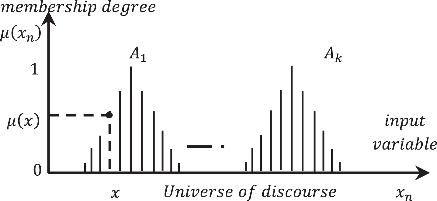
Discrete fuzzification for each x value using triangular functions.
A different approach for representing membership functions is through the use of α-levels to map the different membership values as follows:
An α - level of a fuzzy set A in the form of (3), is a set A
α
defined by the following equation adapted from [25]:
This means that a classical set contains elements of a universe X, represented within a closed interval

Membership function represented withα-levels.
A fuzzy set A could be defined by the union of all its α - levels as follows:
If a fuzzy set A is convex on x axis, its membership functions could be represented by different shapes, such as: Gaussians, trapezoids, triangles, etc., even with non-regular shape. If a membership function or Fuzzy set A is convex on y axis, it cannot be represented byα - levels.
In order to implement the arithmetic digital fuzzifier, some considerations must be done for the discourse universe, the membership degree and the equations of the membership functions used. Each parameter depends on the number of bits used; determining the quantity of computational resources and processing time elapsed by the implementation.
Considerations for the universe of discourse and the membership degree
The variable to control in the process or system must be defined within its discourse universe X, according to the specific application. In the continuous space, the input variable may take either positive or negative values. However, in the discrete space, the variable has to be scaled according to the number of bits used, using either integer or floating point format. The representation with 8-bit integer [0–255] is widely used in digital implementations such as microcontrollers and FPGA’s [26], this format can be found in the works [11, 28]. Then for a n-bit discretization, the universe is represented by a closed interval [0, 2 n - 1].
Similarly the membership degree is also normalized in a continuous space in [0, 1]. In this case, the minimum amount of bits used to represent the membership value is 4-bits [29, 30]. However, more bits can be used, but less than 8-bits since is the worst case for processing. Then for l bits, μ (x) will be in the interval [0, 2 l - 1] in an integer universe. For α - level representation the constraint that l < n in bits must be accomplished since it is the main advantage against the classical fuzzification.
Considerations for the membership functions
The most suitable membership functions for FPGA implementation of fuzzy systems are the trapezoids and the triangles [19]. The trapezoidal function in the continuous space is defined by:
It is to notice that a triangular function is a particularity of the trapezoidal when c = d = 1 in Equation (7). The processing of a triangular function is carried out by piecewise linear functions in the form of (7). Its evaluation implicates two independent arithmetic operations, for the lineal equations for the positive and negative slopes as shown in Fig. 3.
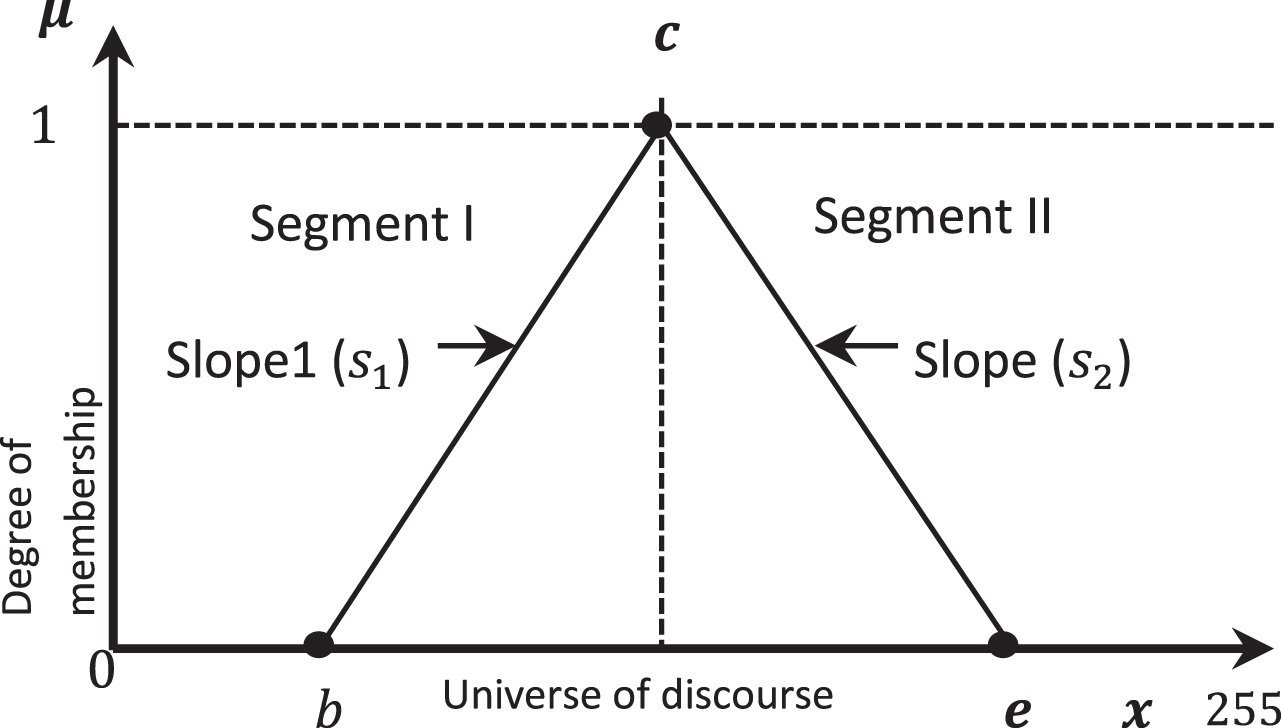
Triangular Type Membership Function.
As the discretization of the discourse universe and the membership with integer numbers does not guarantee integer slopes, these may be expressed as rational numbers in the form of (8) and (9). The Equations (10) and (11) are used for calculating the membership of an input x in the segments I and II respectively. These equations involve subtraction, multiplication and division as shown by [11] and [20]. Also consume much computational resources since the processing of the multiplications and divisions is commonly sequential. Besides, if the membership functions are nonlinear, like Gaussian or sigmoid, then the computational resources and response time are increased.
Given that the division is one of the most resource consuming operation that cannot be expendable, a simplified methodology was presented in [9]. A division 2k/k is calculated by a recurrence equation as in (12)
Where x is the divisor, y the quotient, z the dividend, and s the remainder. This shift-subtract process is repeated until all the k bits of the quotient y have been determined, which implies that k clock cycles are used to complete the operation. Other similar approach is proposed in [31], where the divisor is increased in the double of bits and shifted. The partial remainder is compared with the divisor, if it is greater than the divisor the quotient is “1”, otherwise, the quotient is “0”. If the format is 32 or 64 bits, a larger quantity of clock cycles are necessary.
The proposed fuzzifier is based in the use of α-level and integer numbers for MFs representation. It performs the mapping of the membership universe using 4-bits, in the range [0,15]; and 8-bits for the discourse universe, in the range [0,255]. It was designed for representing triangular or trapezoidal membership functions with positive and negative slopes as in Fig. 4.
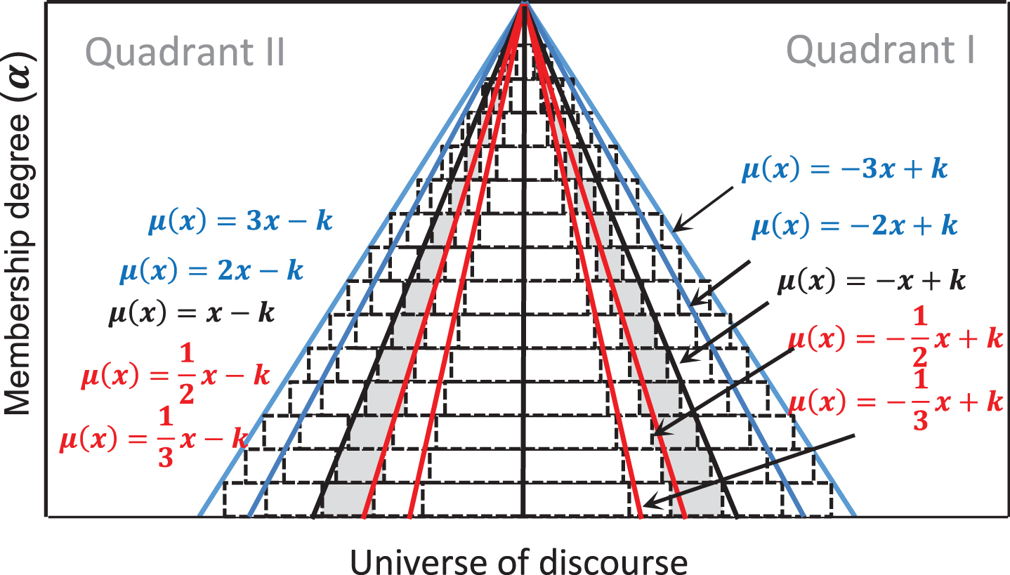
Representation of triangular MFs with α-level.
The representation of a triangular function in the form of (7), includes two linear functions with positive and negative slopes. The positive functions are presented in the quadrant II obtained by μ (x) = qx - k; the negative functions are presented in the quadrant I, obtained by μ (x) = qx + k. When q = 1, we obtain the black triangular function at the center of Fig. 3, with an angle of 45º for the rising slope, and with an angle of 135º for the falling slope.
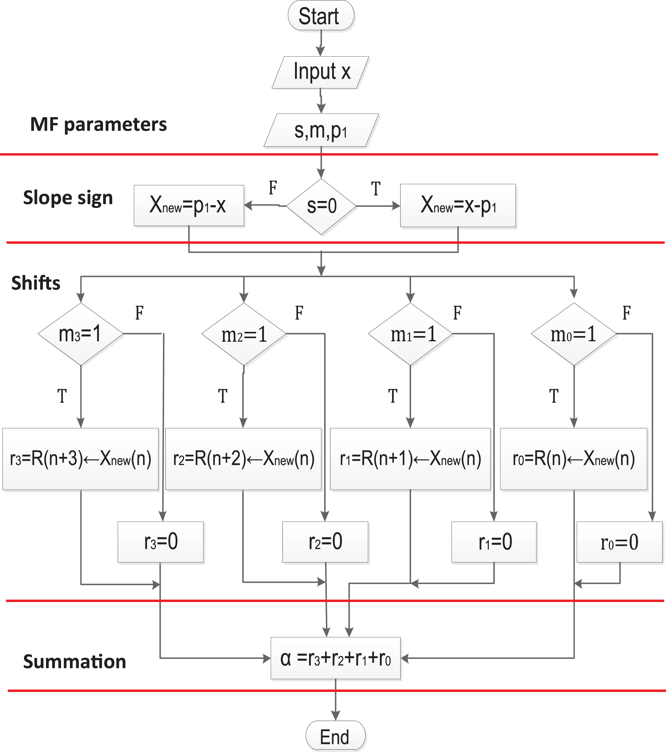
Flow chart for the LSC parallel circuit.
The functions with positive slope can be obtained with integer values of q, getting angles greater or equal than 45° (blue lines in Fig. 4). The functions with slope values lower than 45°, are obtained with rational values of p (red lines in Fig. 4). Is important to notice that in the case of monotonically decreasing functions, i.e. the negative slopes, are a mirror of the positive ones. For implementing the circuits for evaluating an input value x into a membership function A in the form of (7), the circuit must be divided into two blocks according with the value of q. The first block is called logical shift circuit (LSC), and performs the calculations for positive and negative slopes if q is integer. In this circuit, the membership values are calculated by left shifting.
The second block will operate also with positive and negative slopes, but when the values of q are rationale. There are two versions of this block, the parallel and the sequential, called binary search parallel circuit (BSPC) and binary search sequential circuit (BSSC), respectively. Both use the adaptation of the binary search method for calculating the division.
The LSC circuit uses three parameters as inputs: the sign s of the slope (1-bit, 0 for positive and 1 for negative); the slope m (4-bits, for integer values); and the starting point P1, which defines the displacement of the MF from the origin (8-bits). The result of the LSC circuit is the 4-bit value of μ (x) = α, corresponding to the membership value for the given input x. For example, let us assume s = 0, a positive slope; m = 5 (0101, where m3 = 0, m2 = 1, m1 = 0, m0 = 0), the integer value of the slope; P1 = 0, meaning that the MF starts at the origin; and the input to evaluate is x = 2. This value is calculated as follows:
The active bits in m are those with value m i = 1, in this case, the first and the third bits. Therefore, there are two contributing terms: 2 * 20 = 2 and 2 * 22 = 8, that are added to obtain the result. Hence, if the starting point of the function is displaced from the origin, the value of P1 is subtracted from the input variable prior to the calculation. This process is performed in parallel according to the flow diagram shown in Fig. 5. The circuit for the LSC is presented in Fig. 6, where it is possible to identify the three shifters that are executed in parallel, as well as the summation of the partial results.
Combinational architecture of the LSC circuit.
The calculation of fuzzification when the slope is rational requires a more complicated process than with integers. The BSSC circuit realizes sequential processing, and uses an adapted version of the binary searching method. The original algorithm finds a number in an ordered array as well as its memory location. The BSSC circuit looks for a given input x by binary searching, and once it finds it, it provides its corresponding α - level. The BSSC circuit uses as inputs: the sign s of the slope (1-bit); the slope m (4-bits); the starting point P1 (8-bits); the 8-bit left boundary for the interval α = P1; the 8-bit right boundary b; and the 8-bit input x. The result of the BSSC circuit is the 4-bit value of μ (x) = α, corresponding to the membership value for the given input x. Its algorithm is shown in Fig. 7.
Flow chart for the BSSC sequential circuit.
In the BSSC circuit, two registers are necessary to store the limits of the interval [a,b], which is the support of a membership function. The left limit a, is the beginning of the function and may be at the origin ‘0’, but it also may be displaced from the origin, starting in P1. The right limit b of the membership function is calculated using a displacement of b = m * 2 I .
The searching process initiates by dividing the [a,b] interval into the half; the input is compared with the central point c, if the input x is greater than c, then the starting point a is updated as a = c, to use the new interval [c, b]. Otherwise, if the input x is lower than c, then the starting point b is updated as b = c, to use the new interval [a, c]. The process is repeated until finding the value of x on the support of the membership function, when x = c. This process is shown graphically in the Fig. 8.
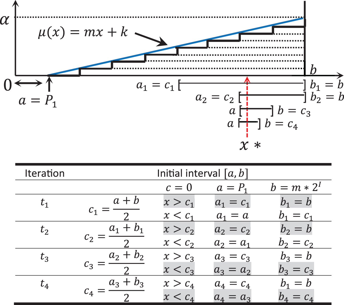
Searching sequence in a lineal membership function (* in gray color).
In a discretized interval of [0,2 l –1], the minimum number of searches is realized in one clock cycle (10 ns), and the maximum number of searches is equal to the number of quantizations l = 4, for this case is four clock cycles (40 ns), in an Artix-7 XC7A100T FPGA.
Figure 9 presents the sequential architecture for the BSSC circuit, which is comprised by five logical blocks. The block INICIO stores the initial values and calculates the support of the membership function. The block SEL_LIMIT calculates the midpoint c of the interval [a,b] and updates the corresponding boundary. The block COMPARA compares the input value x with the midpoint c to determinate the searching sub-interval. The block FSM corresponds to the BSSC control unit. Finally, the block NIVEL, determinates the α-level value.
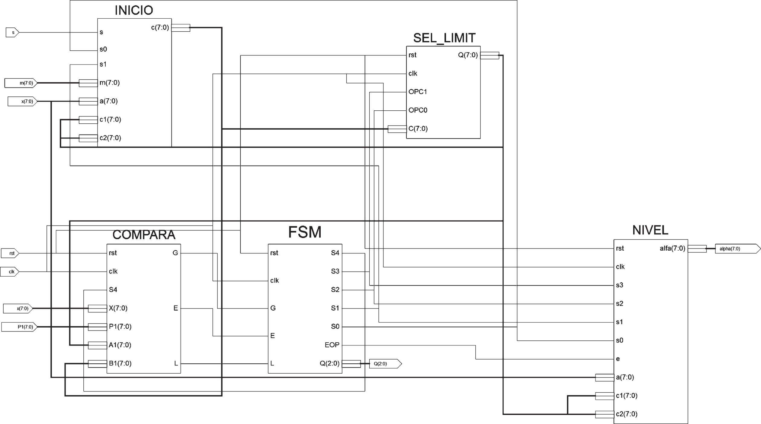
Sequential architecture of the BSSC circuit.
Given that the BSSC circuit implicates a sequential processing, it is desirable to reduce to the minimum the number of clock cycles it takes for processing. Therefore, we proposed a second version of the circuit called BSPC, using the same algorithm but in a parallel architecture.
The BSPC circuit uses as inputs: the sign s of the slope (1-bit); the slope m (4-bits); the starting point P1 (8-bits); and the 8-bit input x. The result of the BSPC circuit is the value of μ (x) = α, corresponding to the 4-bit membership value for the given input x.
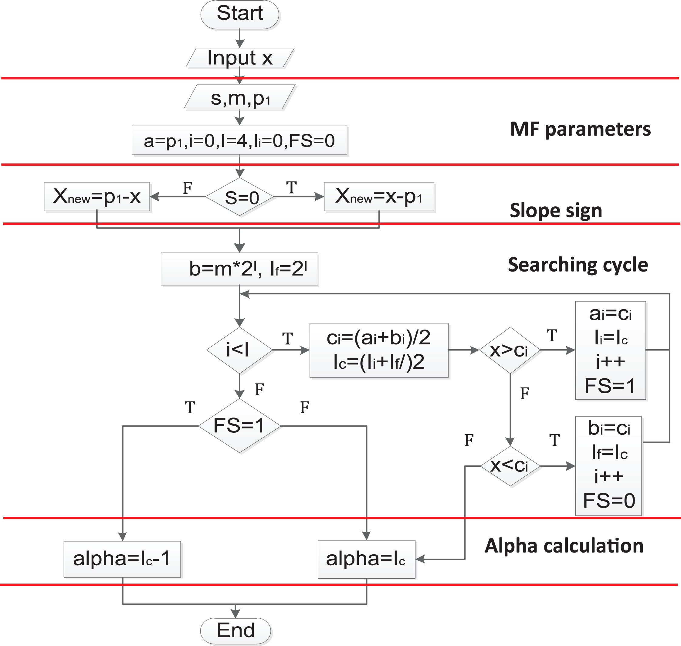
The algorithm is presented in the flowchart at Fig. 10. The first section initializes the membership function parameters like the slope sign, the slope value, and the starting point, and reads the input value. The second section is dedicated to obtain the sign of the slope, assigning the value to X
new
. The next section is dedicated to calculate all the intermediate values out of the slope. This task is done by realizing shifting operations using the base value as in the following equation:
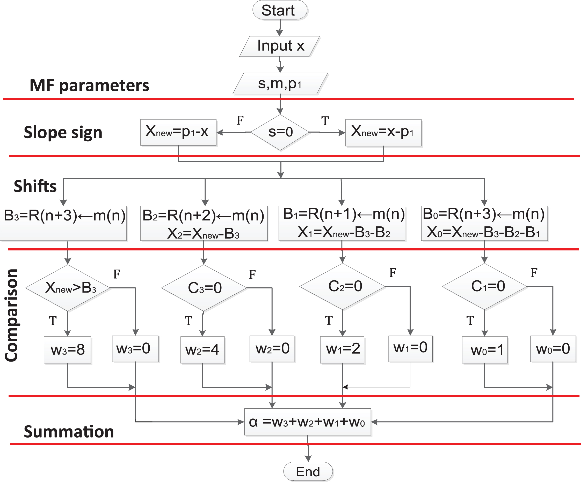
Flow chart for the BSPC parallel circuit.
Note that the number in the parenthesis indicates the amount of shifting, corresponding to the bit weight. Note also that the case of B0, is particular since there is no shifting, then the result could be the input m or zero. In the section labeled as comparison, the input X new is compared first with the calculated B3 intermediate value. If X new is greater than B3, a weight of 2 l = 23 = 8 is generated, otherwise, the result is zero. In this same step, there is a comparison using the carry C2, {C1, and C0) of the previous subtractions where X2, X1, and X0), were calculated in terms of B3, B2, B1, and B0. If the carry is equal to zero, it means that the bit will contribute to the final result and its weight is assigned to w i . The final step is to realize the summation of all the w i to obtain α as result.
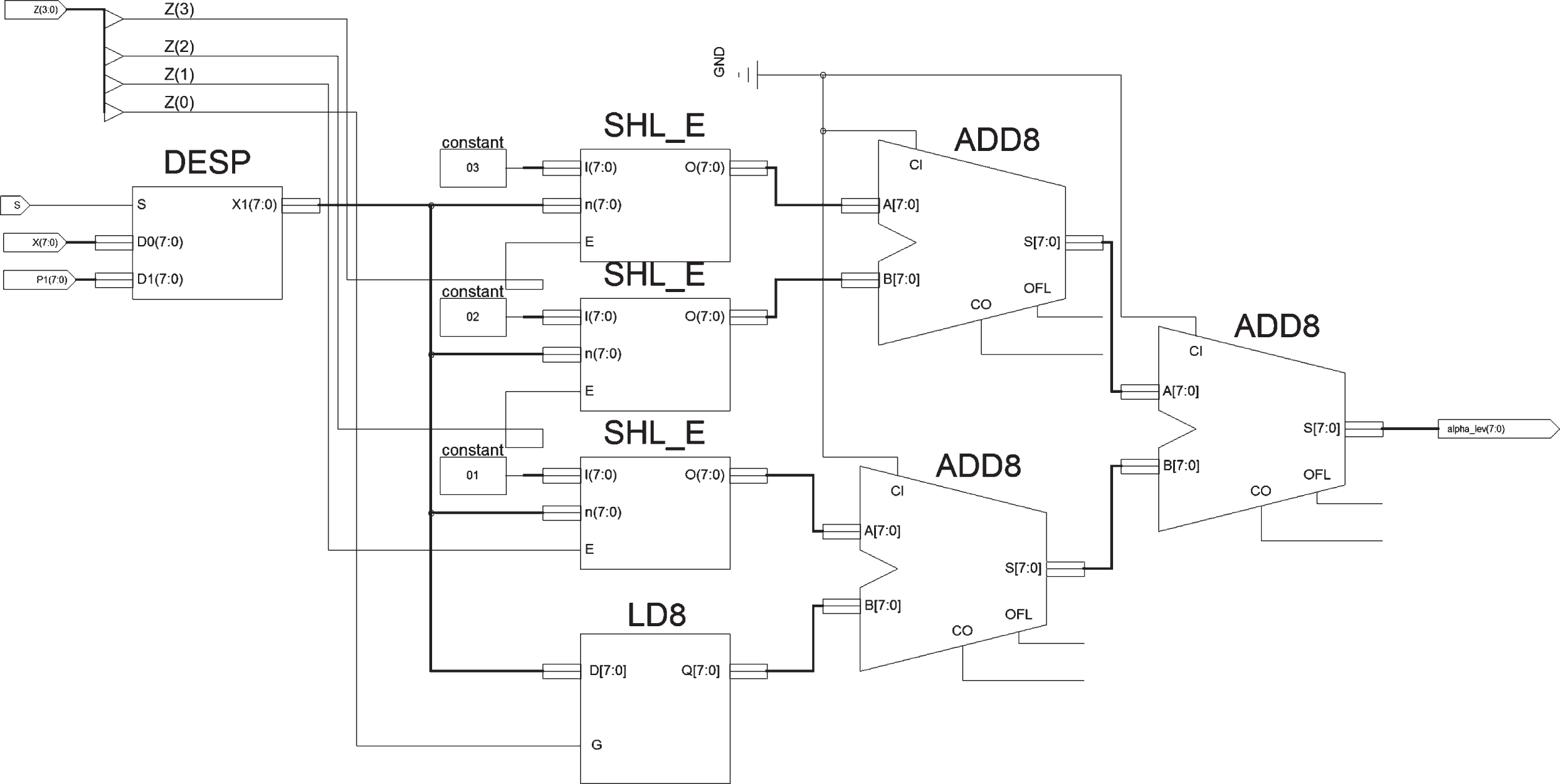
This circuit is also based in the concept of the binary search, but it is not necessary to calculate the central point c between limits a and b, for partitioning the support of the function. The resultant circuit is shown in Fig. 11. The block DESP, calculates the sign of the slope and the value of X new . The block GNRA_U generates the values of B3, B2, B1, and B0. The CMP are the comparators, and the last three blocks calculate the final summation to obtain a.
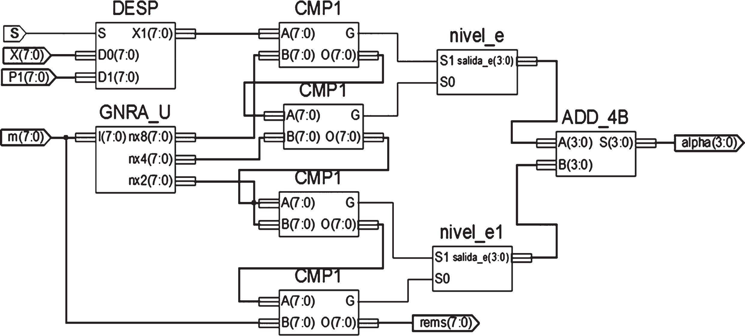
Combinational architecture of the BSPC circuit.
These circuits were implemented in an Artix-7 XC7A100T FPGA, through the schematic design for all combinational and sequential circuits that make up the architecture of the fuzzifier. The test results were performed by using the ISIM library of the development environment ISE 14.2. Each circuit was simulated individually by using the linguistic variable A, which is composed of three triangular membership functions (15)–(17), usually used for controlling position in a DC motor, represented in a-levels, (horizontal lines) as shown in Fig. 12.
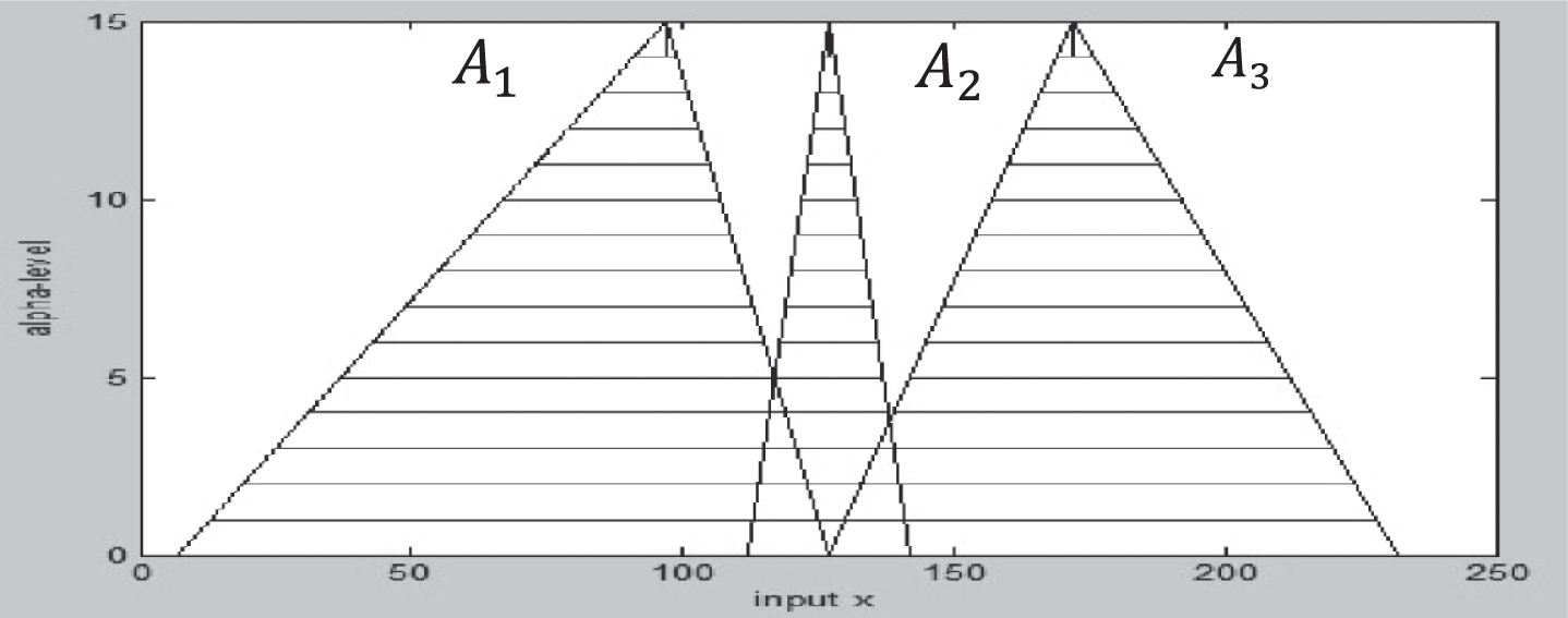
Membership functions used for simulations.
The simulations for the three circuits (LSC, BSSC and BSPC) present the following common signals: s is the sign of the slope, m is slope either integer or rational, P1 is the starting point of the membership function, x is the input value and alpha is the output of the fuzzification circuits. The signal s = 1 indicates that the circuit will operate with a negative slope, when s = 0, the slope is positive.
Figure 13, presents the performance of the LSC, BSSC and BSPC circuits (dashed line) versus the fuzzification in floating-point (solid line) for 100 input values. The testing of the fuzzification circuits is as follows: the BSSC circuit is evaluated by A1; the LSC circuit by A2; and finally the BSPC by A3. Note that the discrepancy of fuzzification in the MF A2 is less than A1 and A3. The simulation results for the LSC circuit are shown in Fig. 14, in which different input values were tested, obtaining their membership, corresponding to the highest a-level reached. Note that the results are available as soon as the signals are propagated through the circuit, in 7.155 ns.

LSC, BSSC and BSPC circuits vs. Floating-point fuzzification.
Simulation performance of the LSC circuit.
The simulation results for only three inputs for the BSSC circuits are shown in Fig. 15. Due to its sequential processing, it uses the signal rst to reset the circuit to initial conditions when rst = 1. The row labeled as clk is the clock signal that activates the data load in the rising edge. It starts the calculations that take four clock cycles to have a result, which is indicated by the eos signal (end of searching) and the yellow dashed line.

Simulation for the performance in the BSSC circuit with different inputs. (a) x = 60, (b) x = 84, (c) x = 71.
This block was evaluated with some input values. The simulation results are shown in Fig. 16, note that the result is obtained immediately after the input is fed into the circuit, having a propagation time of 14.912 ns.

Simulation of the performance in the BSPC circuit.
One of the purposes of this fuzzifier is to reduce the response time; hence, the parallel processing is a suitable option to achieve this goal. There are two architecture options to realize the complete fuzzifier out of the presented blocks, since the LSC block works with integer slope values and the BSSC and the BSPC works with rationale values. The LSC + BSSC option is the sequential, and the case of LSC + BSPC circuits, performs its calculations in parallel. However, the configuration that performs the calculation with a better response time is the LSC + BSPC parallel circuit. This array is called a-level Based Binary Search and Shifting Fuzzifier a-BSSF.
The simulation for the whole fuzzifier circuit is carried out using a linguistic variable with two triangular membership functions: μ
slow
(x) and μ
fast
(x), represented in α - levels. Both variables are defined by segments as in the Equations (18) and (19) and are graphically represented in the Fig. 17.

Triangular membership functions for Fuzzification with α - BSSF.
The testing of the α - BSSF circuit was realized using different parameters, as presented in Table 1. The first two columns present the slope and displacement for the segments of the membership functions as in (18) and (19). The third column shows the input values for x, while the fourth column indicates in which MF is evaluated. The fifth column indicates the membership result delivered from the circuit, while the last column indicates the membership value obtained analytically for each input x. It is important to notice that the method allows only two overlapped functions.
Parameters for testing the α - BSSF circuit
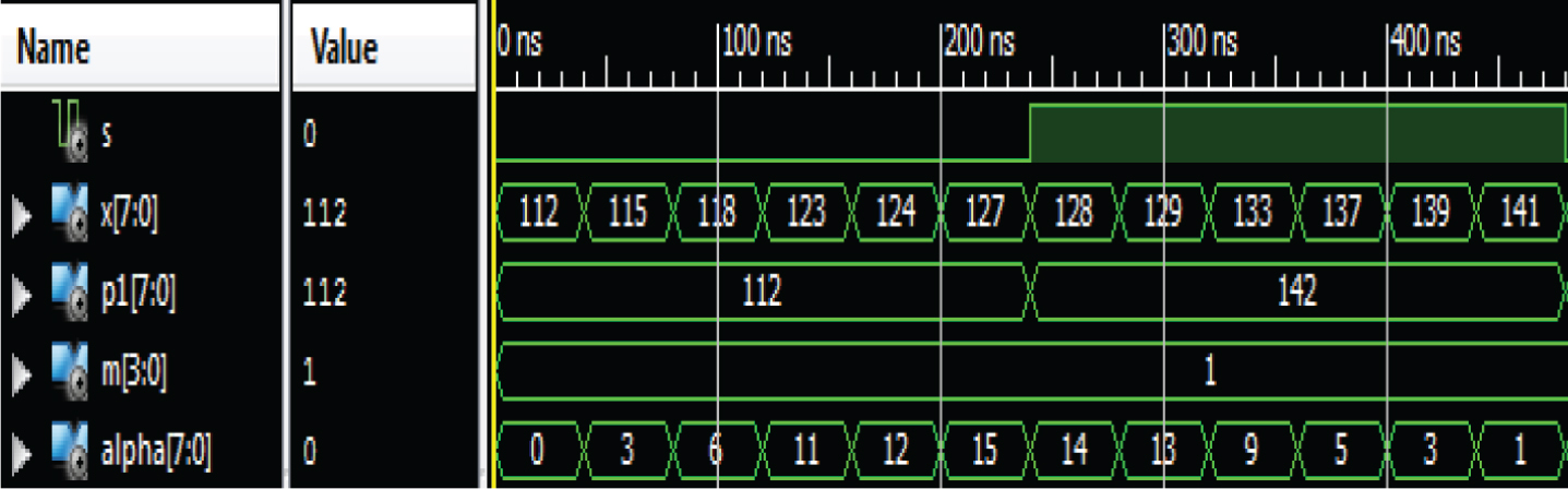
The simulation results of the α - BSSF circuit are shown in Fig. 18. The first row called ′s0′, corresponds to the slope, which switches from positive and negative slopes. The second row, contains the values for the input x, with a holding time of 40 ns each one; and the third row presents the values for the displacement P1. The results of the fuzzification are shown in the last row called alpha, The result is available as soon as the input values are propagated in a time of 15.853 ns.

Simulation for the Fuzzification in the α - BSSF circuit.
There is a notorious importance in the use of binary division in the calculation of arithmetic fuzzification in the form of (8) and (9), since it directly affects the response time. There are different division algorithms that could be realized in sequential or parallel architectures. The sequential architectures generate a result after several clock cycles, while the parallel ones requires only the propagation of the signals to complete the operation [32]. The parallel algorithms use a larger number of computational resources compared to the sequential ones, however, the processing with integer operations, that are simpler than in floating point, implicates another reduction in resource consumption [33]. For our case, only the integer part is considered and the parameter s will be despised.
Table 3, presents the synthesis results of the implementation of the BSPC algorithm in an XC7A100T FPGA, comparing its resource consumption against the DSS circuit proposed in [9] and the DBI circuit from [31]. The columns shows the amount of slice registers used by each circuit, the number of slices of Look-Up Table’s (LUT) used, the occupied slices and the time required to complete the operation.
Resources consumed by the BSPC circuit
Resources consumed by the BSPC circuit
Resource consumed by α - BSSF circuit
The BSPC circuit does not use slice registers, and the DBI circuit uses 86% less slice registers than the DSS. For the LUT Slice consumption, the BSPC circuit, increases the consumption in 13% against DBI, and reduces its consumption in 53% against DSS. Regarding the number of occupied slices, the BSPC, reduces its number in a 20% against the DBI and 47% against the DSS.
The most outstanding characteristic of the BSPC is that it performs the division in parallel obtaining the result as soon as the signals are propagated trough the circuit in 14.912 ns. The sequential circuits DSS and DBI perform their calculation in 4 and 8 clock cycles respectively.
There are many digital implementations of fuzzifiers for T1FS, either in the arithmetic or pre-calculated approach. However, since most of them share computational resources with other functional blocks in a fuzzy controller, it is difficult to find the values for the response time or the clock cycles used in this independent block. Table 3, presents the resources consumed by the implementation of the α - BSSF Fuzzifier, which is comprised of the LSC + BSPC circuits. It also presents the sequential option which is comprised of the LSC + BSSC circuits, both configurations were implemented in an Artix-7 XC7A100T FPGA.
The resources consumed by the α - BSSF parallel circuit against the LSC + BSSC sequential circuit, are 86% less slice registers used, 52% less LUTs and 63% less occupied slices. Also, note that the processing speed for the α - BSSF circuit is 2.7 times faster.
With the purpose of making a fair comparison of the resources used in the LSC + BSSC and the α - BSSF circuits, against other existing proposals, it was necessary to make an implementation in an older FPGA, the Spartan 3 XC3S50 FPGA. This is because we want to compare these circuits against the ones presented in [34, 35] and an additional work [18], which are implemented in this FPGA. Table 4 presents this comparative. The first columns indicates the tested circuit; the second column shows the number of slice latches used by each circuit; the third column indicates the number of 4 LUTs used; the number of occupied slices consumed are indicated in the fourth, the total utilization of resources is presented in the fifth column and finally, the operation speed in cycles or processing time is shown in the sixth column.
Resource consumed by fuzzifiers in XC3S50 FPGA
Resource consumed by fuzzifiers in XC3S50 FPGA
The Table 4 summarizes the resource consumption for different fuzzifiers. Only four implementations report processing time, these designs are based in triangular, trapezoidal or Gaussian memberships. The designs with higher resource consumption are the multi-function fuzzifier from [34] with 57%; and the proposed LSC + BSSC with 62%, by performing a sequential calculation. The circuit in [39] present the lowest resource consumption, unfortunately, the response time is not provided; the proposed parallel circuit α - BSSF presents a 28 % of utilization. The cases [35, 36] and [37] have an average of 40% in resource consumption. The circuits with highest processing time are in [39], with 401 ns, and the sequential LSC + BSSC with 80 ns. The lowest propagation time is 13 ns, is presented in [18], and with a similar value is the α - BSSF, the main difference is that the last design is tested at a lower clock frequency.
Finally, the circuit, which presents the best equilibrium between resource consumption, processing time and the flexibility for defining membership functions, is the proposed α - BSSF circuit.
In order to evaluate the accuracy of the α - BSSF fuzzifier is necessary to calculate its deviation against two analytical approaches: the arithmetic in floating-point representation, being the reference measure, and its fixed-point representation. The first representation is the one that is calculated manually at theoretical courses, while the second is an approximation of the first one, targeted for hardware implementations.
The Root Mean Square Error (RMSE) is used to determinate the accuracy of the α - BSSF design, and it is calculated as follows:
Where n is the number of samples; f i is the result of the fuzzification with integer numbers, and fi FP is the result of the arithmetic value calculated in floating-point format. The input values x were computed using the membership functions in the Fig. 16 with n = 100 samples. Is important to note that the floating-point fuzzifier provides the ideal result, and will be used as reference.
The α - BSSF fuzzifier, uses 8-bits in the universe of discourse as mentioned in section 3. For normalizing the RMSE, we used the boundaries x
min
= 0 and x
max
= 255 as follows:
For comparison purposes, we also used a fixed-point fuzzifier with word length of 8-bits and a fractional length of 4-bits. The results for the NRMSE are presented in Table 5. The fuzzification results for floating point, fixed-point and the α - BSSF are shown in the Fig. 19 (a). The error percentages for the fixed-point and α - BSSF for different values of x are plotted in Fig. 19 (b).
NRMSE for different fuzzifiers
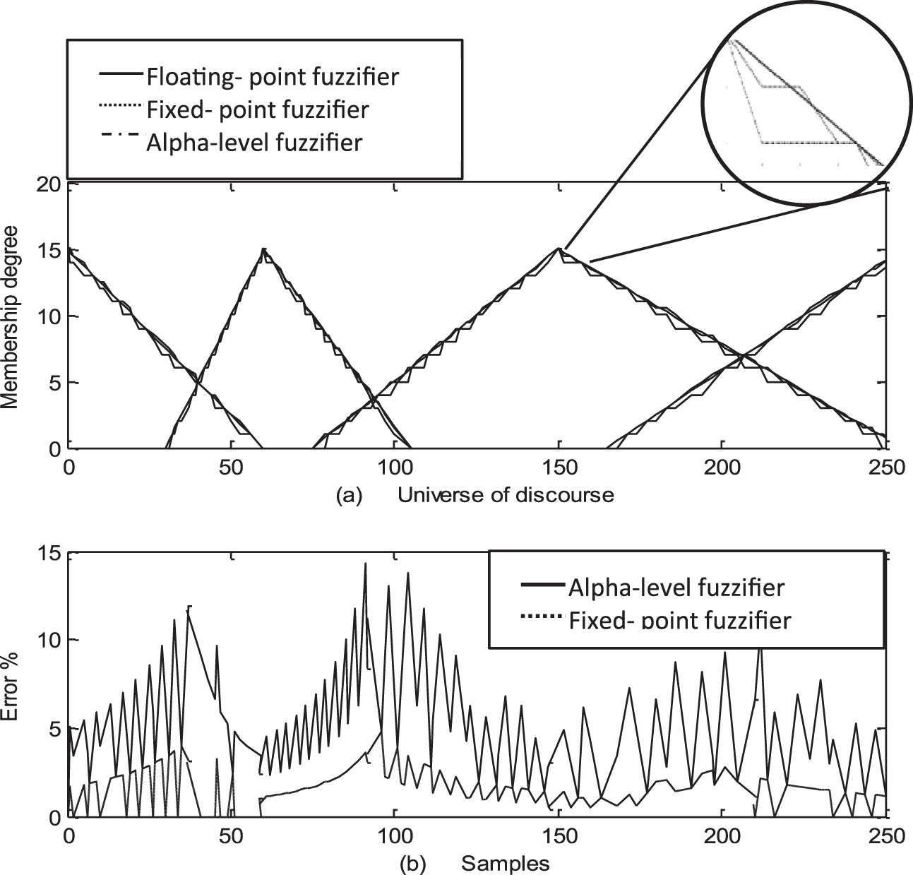
(a) α - BSSF Circuit vs. Floating –point Fuzzifier, (b) Error percentage of the fixed-point vs α - BSSF fuzzifier.
The work presented by [18] shows the architecture of a Dynamic Precision Fuzzifier with a value of NRMSE of 0.00016 and a traditional block with error of 0.00019. Notice that the difference between them is very close, even is less than the error of a traditional Fixed-point.
The NRMSE generated by the circuit is 0.00209, which correspond to a very acceptable value for a fuzzifier that uses processing with integer values, which is used by many controllers as in [15, 41].
Currently most of the Type-1 fuzzification blocks are implemented either with the arithmetic approach in running time or the storage of pre-calculated values using a memory circuit. Both methods implicate the usage of multiplication or division and it is not very common to find reconfigurable implementations. The proposed α - BSSF fuzzifier circuit is a logic block, which could be used in the calculation of membership degree trough α - levels, or in arithmetic operations of multiplication and division in the process of classical fuzzification.
When the computational resources are an important issue in FPGA implementations, the use of triangular and trapezoidal function are a good option to use due to its simplicity and desired results in fuzzy hardware.
The main advantage of the α - BSSF is the response time, given its parallel architecture, which is reflected in a higher quantity of information processed in less time.
The α - BSSF fuzzifier could be used in any existing fuzzy logic controller architecture based in FPGA or even by 8-bit soft core microcontrollers. Additionally, it can be scaled up to perform calculations with greater bit size.
The applicability of the α - BSSF is not limited to T1FS, since the fuzzification process in T2FS involve the same calculations but repeated twice for the upper and lower membership functions. So the same circuit could be used in T2FS.
Footnotes
Acknowledgments
The authors would like to thank the Instituto Politécnico Nacional and the CONACYT for their financial support in the realization of this project.