An algorithm for computing the generalized interaction index for k -maxitive fuzzy measures

Abstract

Fuzzy measures are used for modeling interactions between a set of elements. Simplified fuzzy measures, as k-maxitive measures, were proposed in the literature for complexity and semantic considerations. In order to analyze the importance of a coalition in the fuzzy measure, the use of indices is required. This work focuses on the generalized interaction index, gindex. Its computation requires many resources in both time and space. Following the efforts to reduce the complexity of fuzzy measure identification, this work presents two algorithms to compute the gindex for k-maxitive measures. The structure of k-maxitive measures makes possible to compute the gindex considering the coalitions at level k and, for each of them, the number of coalitions sharing the same coefficient (called inheritors). The first algorithm deals with the space complexity and the second one also optimizes the runtime by not generating, but only counting, the number of inheritors. While counting the number of descendants is easy, this is not the case for the number of inheritors due to all the inheritors of previous considered coalitions have to be taken into account. The two proposed algorithms are tested with synthetic k-maxitive measures showing that the second algorithm is around 4 times faster than the first one.

Keywords

Fuzzy measures Shapley index interaction index

1 Introduction

Fuzzy measures were proposed by Sugeno [20] to generalize probability measures by relaxing the additivity axiom with a monotonicity constraint. The ability of fuzzy measures to model the interaction among subsets of a set N = {X₁, …, X_i, …, X_n} make them suitable for diverse fields of science like biology [17], economics [9], computer science [28], decision making [22 , 27], to name a few.

Despite the descriptive power of fuzzy measures, their practical application is limited by the complexity of their coefficient identification: n elements require the evaluation of 2ⁿ-2 coefficients. This exponential growth is their Achilles’s heel, restricting their use to problems with a handy number of elements. Although there are many algorithms to identify the 2ⁿ elements of the fuzzy measure [1 , 24], they are limited to small values of n. In an attempt to achieve identification scalability, simplified fuzzy measures have been proposed based on the inclusion of new restrictions. The λ-measure [21] reduces the number of coefficients to be identified to n + 1: singletons and λ, but this simplification goes along with a loss in modeling capability. A trade-off between complexity and modeling capability is proposed by measures that model the interaction between at most k elements, including k-additive [3] and k-maxitive [11, 12] measures. The use of k-maxitive measures instead of general fuzzy measures is supported by semantic and complexity considerations [14]. Coefficients of k-maxitive measures are identified for coalitions of cardinality up to k, the ones with cardinality between k and n are set based on those already identified.

This simplification reduces the space and time complexity of the identification algorithm: only values for coalitions with cardinality up to k are identified and stored.

The coefficient μ (A) associated with a coalition A considering a fuzzy measure μ may be interpreted as a weight assigned to the coalition A. However, since fuzzy measures are constrained by monotonicity, a more precise characterization of A contribution to the set N cannot be directly deduced from μ (A). In the field of cooperative game theory, Shapley [19] proposed an index to characterize individual contributions. The index was first generalized to pairs of elements [16] and then, to subsets of arbitrary cardinality through the gindex [3].

The collective behavior characterization is a key point in problems where individual considerations may not be statistically significant. Through gindex, behaviors such as complementary or redundancy among elements can be evaluated [15].

The classical computation of the gindex includes two summations. All the subsets of N are considered in the formula (in the first or second summation) and their individual generation is not a straightforward. But it is possible to rewrite the formula with only one summation [4], which makes the generation of all elements in $ℙ (N)$ simpler. In any case, its computation has the same complexity as the fuzzy measure.

Although the indices provide useful information about interactions of coalitions, their computation may require an important effort. Some algorithms to compute the Shapley index on special situation [8] or to compute other indices [18, 25], were proposed but none of them makes the most of the structure of k-maxitive fuzzy measures. Following the efforts to reduce the complexity of fuzzy measure identification, the motivation for this work is to achieve a similar reduction in the calculation of the gindex. The objective of this work is twofold. Firstly, a new algorithm to compute gindex for k-maxitive measures is introduced. This new algorithm, naive kindex, uses the formula with only one summation and an easier way for subset generation. It also introduces several improvements to reduce the complexity. Secondly, to take advantage of the underlying structure of k-maxitive measures, a second algorithm, kindex, is presented. All the coalitions that share the same coefficient are considered at the same time. In this way, their contribution to the gindex is computed without individualizing all their elements, i.e., not all the coalitions are generated.

A complexity analysis is carried out for the two proposed algorithms. Finally, time requirements are evaluated using synthetic k-maxitive measures.

The outline of this work is the following: Section 2 introduces basic concepts related to fuzzy measures and their representation, Shapley index and k-maxitive measures. Section 3 presents two approaches to compute the gindex from a k-maxitive measure. In Section 4, the complexity of the two proposed algorithms is analyzed. In Section 5 optimization enhancements are presented and both algorithms are tested with synthetic k-maxitive measures. Finally, Section 6 presents the conclusions and open perspectives.

2 Preliminaries

Let N = {X₁, …, X_i, …, X_n} be a finite set and $ℙ (N)$ its power set. In what follows, lower case letters represent the cardinality of the set denoted by same letter in uppercase, s=|S|.

2.1 Fuzzy measures and their representation

Definition 1. A fuzzy measure is a set function $μ : ℙ (N) \to [0, 1]$ fulfilling the following two axioms:

μ (∅) =0, μ (N) =1

A ⊆ B ⊆ N ⇒ μ (A) ≤ μ (B)

The first axiom, called the normalization axiom, allows for meaningful comparisons between fuzzy measures. The second axiom formalizes a monotony constraint. The numbers μ (A), called the coefficients of the measure μ, are the weights given to the elements of $ℙ (N)$ .

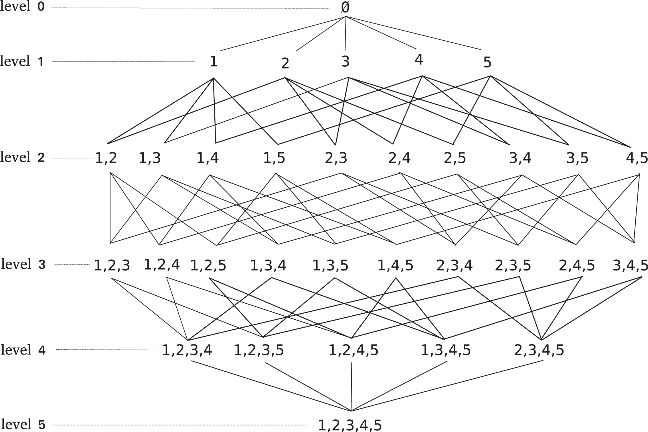
A suitable way of representing fuzzy measures in the finite case is through a lattice. $ℙ (N)$ is a lattice ordered by inclusion. Subsets with the same cardinality are mapped to vertices in the same lattice level and their cardinalities can be used to identify such levels. Hence, while the lattice level labeled with 0 will contain only the empty set ∅, the lattice level labeled with n will contains the whole set N (see Fig.1).

Fig. 1

A lattice representation of $ℙ (N)$ with N = {X₁, X₂, X₃, X₄, X₅}. Element X_i is represented by vertex i and subset {X_i, X_j} by vertex i, j.

Definition 2. The neighbors of a lattice vertex at level l are the vertices connected to it at levels (l-1) and (l+1).

Definition 3. A subset U at level h of the lattice is an ancestor of a subset V at level l > h if U ⊂ V.

Definition 4. A subset W at level d of the lattice is a descendant of a subset V at level l < d if V ⊂ W.

2.2 Shapley index

The Shapley index of an element X_i ∈ N [19] is calculated as follows: $φ ({X_{i}}) =$ (1) $\sum_{Z \subseteq N \ {X_{i}}} \frac{(n - z - 1)! \cdot z!}{n!} \cdot (μ (Z \cup {X_{i}}) - μ (Z))$ where 0!=1 as usual. The Shapley value of a fuzzy measure μ is the vector φ = [φ ({X₁}) ⋯ φ ({X_n})] and satisfies: $\sum_{i = 1}^{n} φ ({X_{i}}) = μ (N) = 1$ (2) The generalization of the Shapley index, called gindex, for sets of arbitrary size is shown in Eq. (3). $gindex (A) =$ (3) $\sum_{Z \subseteq N \ A} \frac{(n - z - a)! \cdot z!}{(n - a + 1)!} \sum_{B \subseteq A} (- 1)^{a - b} \cdot μ (Z \cup B)$

The computation of the gindex for a set A in Eq. (3) comprises two parts, each of which includes a summation. The first one, considers all subsets Z of the set N \ A, i.e., $Z \in ℙ (N \ A)$ ; and the second one, all subsets B ⊆ A, i.e., $B \in ℙ (A)$ . The first part performs a normalization and, in the second one, the union of the two sets, Z and B, is weighted according to the cardinalities of A and B measuring the contribution of all possible subsets of A in all possible subsets of N \ A.

It is possible to rewrite Eq. (3) as follows [4]: $gindex (A) =$ (4) $\sum_{I \subseteq N} (- 1)^{(a - b^{'})} \cdot \frac{(n - z^{'} - a)! \cdot z^{'}!}{(n - a + 1)!} \cdot μ (I)$ where b′ = |I ∩ A| and z′ = i - b′. Eq. (4) does not involve any set union and has only one summation.

2.3 k-maxitive measures

The possibilistic Möbius transform [2] of a fuzzy measure μ on N is a mapping $m_{p} : ℙ (N) \to [0, 1]$ defined by: $m_{p} (A) = {\begin{matrix} μ (A) if μ (A) > max_{B \subset A} μ (B) \\ 0 & otherwise \end{matrix}$ (5)

Definition 5. A fuzzy measure μ is called k-maxitive if its possibilistic Möbius transform satisfies m_p (A) =0 for any A such that a > k and there exists at least one subset A of N with exactly k elements such that m_p (A) ≠0.

A way to design a k-maxitive measure is to set the coefficients μ (A), for a > k, to the maximum coefficient value of the k-size subset included in A as stated in Eq. (6). $\forall L \subset N, l > k, μ (L) = max_{S \subset L s = k} μ (S)$ (6)

Definition 6. A subset I is an inheritor of a subset V in a k-maxitive measure μ if I is a descendant of V and μ (I) = μ (V).

Note that, unlike the concept of descendant, this definition requires a measure. Therefore, this definition is more restrictive than Definition 4. Let us assume N=5 as in Fig.1 and a 2-maxitive measure where μ ({1, 2}) > μ ({1, 3}) > μ ({1, 4}) > ⋯ > μ ({4, 5}). Coalition {1, 2, 3} is a descendant of coalitions {1, 2}, {1, 3} and {2, 3}. Moreover, since μ ({1, 2}) > μ ({1, 3}) > μ ({2, 3}) then {1, 2, 3} inherits from {1, 2}, i.e., μ ({1, 2, 3}) = μ ({1, 2}). While counting the number of descendants is easy, this is not the case for the number of inheritors. This is a key point the proposed algorithm has to tackle.

Notation. As subsets of N are used in different contexts in this paper, the word coalition is used to refer to elements in the domain of the fuzzy measure or those for which the interaction index is computed, and the word subset is used for any other general purpose.

3 gindex computation from k-maxitive measures

The computation of the gindex can benefit from the particular structure of k-maxitive measures. In this case, only coefficients up to level k are individually set and those of levels l > k are derived from the ones at level k.

Two algorithms are proposed. Both of them assume that the coefficients associated with coalition of cardinality greater than k are not stored in memory to reduce space requirements [14]. In the first algorithm, each coalition of level higher than k is generated and its coefficients computed “on the fly”. In the second one, the coalitions higher than k are not even generated.

3.1 First approach: a naive implementation

One alternative to compute the gindex from a k-maxitive measure is to replace the function μ in Eq. (4) with the function μ^* in Eq. (7): $μ^{*} (I) = {\begin{matrix} μ (I) & if i \leq k \\ max_{S \subset I s = k} μ (S) & if i > k \end{matrix}$ (7)

The calculation of the gindex using Eq. (7) is implemented in Algorithm 1.

Algorithm 1 naive kindex

1: Input: C: all coalitions, n the number of elements, A ∈ C, μ: a k-maxitive fuzzy measure

2: Output: gindex (A).

3: for I: ∈ C do

4: b′ ← |I ∩ A|

5: z′ ← i - b′

6: if i ≤ k then

7: m ← μ (I)

{store coefficient}

8: else

9: $m \leftarrow \max_{s = k} {μ (S) : | S \cap I | = s}$

{max of coefficient at level k included in I}

10: end if

11: $w \leftarrow \frac{(n - z^{'} - a)! \cdot z^{'}!}{(n - a + 1)!}$

12: sum ← sum + (-1) ^(a-b′) · w · m

13: end for

14: return sum

$C = ℙ (N)$ to compute the gindex (A), but it is possible to consider only a subset of $ℙ (N)$ which is useful for the next approach.

This modification introduces, for all coalitions I ∈ C and i > k, the search for the maximum over all coefficients associated with coalitions contained in I at level k (Line 9 and Eq. (6)). Lines 6, 8, 9 and 10 are specific to k-maxitive measures, they are not needed for general fuzzy measures, i.e., when all the coefficients are stored.

When computing the gindex using this approach, all the coalitions are generated (Line 3) so that the complexity was reduced in terms of space but not in terms of time.

3.2 Second approach: counting instead of generating

In a k-maxitive measure, all the inheritors of a coalition at level k share the same coefficient. Then, their contribution to the gindex could be computed knowing the coefficient (the same for all of them) and their total number, avoiding their generation. The idea is to divide the gindex calculation into two parts: in the first part, the contribution to the gindex of coalitions from level 1 to k is computed as usual using Eq. (4) (through naive kindex). In the second part, the number of inheritors of each coalition at level k is counted and their contribution to the gindex computed. The count of the inheritors is performed level by level since the inheritors share the same coefficient but the normalization factor depends on the level.

3.2.1 gindex algorithm for k-maxitive fuzzy measures: kindex algorithm

The calculation of the gindex from k-maxitive fuzzy measures is presented in Algorithm 2. The input of the algorithm is a finite set of elements N, a coalition $A \in ℙ (N)$ and a k-maxitive fuzzy measure. The output is the value of gindex (A).

Algorithm 2 kindex

1: Input: N: a set of elements; $A \in ℙ (N)$ ; μ: a k-maxitive fuzzy measure.

2: Output: gindex (A).

3: sum← naive kindex(C, n, A, μ)

{contribution of all $C \in ℙ (N)$ where c ≤ k}

4: v ← Sort (k, μ)

{sort coefficient at level k in decreasing order}

5: T ← N

6: for J ∈ v do

7: for B ⊆ A do

8: if |A ∩ J| > |B ∩ J| then

9: next B

10: end if

11: b′ ← |B|

12: for l ∈ (k+1) ⋯ (n-1) do

13: z′ ← l - b′

14: $w \leftarrow \frac{(n - z^{'} - a)! \cdot z^{'}!}{(n - a + 1)!}$

15: qty ← InheirCount (J, B, l, T)

{uncounted inheritors of J at level l}

16: sum ← sum + qty · (-1) ^(a-b′) · w · μ (J)

17: end for

18: end for

19: T ← Split (T, J)

{split all elements of T containing J}

20: end for

21: return sum

The first part of the algorithm computes the contribution of the coalitions up to level k using Algorithm naive kindex (Line 3). After that, coalition-coefficient pairs at level k are sorted in descending order of coefficients and saved in vector v (Line 4). Uncounted inheritors can only be generated from the elements in collection T (Line 5), this is explained in details in subsection 3.2.2. The main loop (Lines 6-20) calculates the contribution of each coalition J ∈ v at level k and its inheritors to the gindex.

The computation of Gindex (A) involves two types of subsets as stated in Eq. (3): the subsets of A, called B, and the subsets of the complement of A in N: $ℙ (N \ A)$ . Although the coefficients of inheritors of an element are equal, their contribution to the gindex is affected by the normalization factor (w) and the sign ((-1) ^(a-b′)) (Line 16). For a certain level, the value of b′ of the inheritors may be different (see Eq. (4)) and then, the B subsets must be considered individually. The inheritors of J can be then written as {{J \ A} ∪ {B}} ∪ {N \ {J ∪ A}}. The first set considers all the subsets of A to assign the specific b′ (Line 11). Even if the assignment differs from the one in Algorithm 1 (Line 4), the same symbol is used because it represents the same information: the number of elements of A for the set that is being examined.

The coalitions at level k (Line 6) may include some elements of coalition A, then, when B ⊆ A (Line 7) there is no need to consider some subsets of B, this is stated by the test condition to be satisfied: |A ∩ J| > |B ∩ J|. The following example illustrates the possible situations.

Illustrative example Let N = 5 as in Fig.1, k=2 and A = {1, 2}. |A ∩ J| can take the values 2, 1 or 0. For J={1, 2} |A ∩ J|=2, then only B={1, 2} has to be considered (Lines 8-10). The inheritors are all the subsets including {1, 2} with all the combinations of {3, 4, 5}, 7 coalitions in levels 3, 4 and 5 (see Table 1). In this case where J={1, 2}, {{J \ A} ∪ {B}} = {1, 2} and {N \ {J ∪ A}} = {3, 4, 5}. It does not make sense to consider B={1} since element {2} must be necessarily present in the inheritors (it belongs to J), i.e., element {1} with any combinations of {3, 4, 5} are not descendants of {1, 2}. If the next coalition to be analyzed is J={2, 3}, |A ∩ J|=1 and both B={1, 2} and B={2} have to be considered. In the former case, the inheritors are all the subsets including {2, 3} ∪ {1, 2}={1, 2, 3} with all the combinations of {4, 5}, however, all of them were already counted when J={1, 2} was considered. Then, B={2} is considered and the inheritors are all the subsets of {2, 3} ∪ {2}={2, 3} with all the combinations of {4, 5}, 3 coalitions at level 3 and 4 (see Table 2).

The value of z′ (Line 13) depends on the level: it is the number of elements in J that do not belong to A. The weight of J (Line 14) is computed using the value of z′. Subroutine InheirCount identifies sets in T which includes {{J \ A} ∪ {B}}, i.e., T_i ⊃ {{J \ A} ∪ {B}} and counts the inheritors of J at level l (Line 15). The way InheirCount counts inheritors using formula (8) and T is explained in subsection 3.2.3. The contribution of J and its inheritors to the gindex is calculated and the weighted sum is updated (Line 16). Finally, collection T is updated through Split function so that J can not be generated again from any of the sets in T (Line 19).

3.2.2 Method to avoid counting associated inheritors more than once

The determination of the number of descendants of an element at level k is given by $\sum_{i = k + 1}^{n} (\begin{matrix} n - k \\ i - k \end{matrix})$ . But the number of inheritors is equal to the number of descendants in only one case: for the highest (first analyzed) coefficient associated with a coalition of cardinality k. Once the highest coefficient is considered, all the other coalitions at level k will share descendants with it and a smaller number of inheritors since they were already counted. Then, for the next steps, the subsets that inherited previous coefficients must be subtracted from the number of descendants.

To count the number of inheritors, the coefficients at level k are sorted in decreasing order. A collection of sets, named T, is used to avoid counting coalitions already counted. At the beginning of the process T = {N}, meaning that it includes only one set, the one that includes all the elements. Then, the first step consists in counting the number of descendants of the coalition with the maximum coefficient value: all descendants are inheritors, their number at level l is $(\begin{matrix} n - k \\ l - k \end{matrix})$ . To ensure that the analyzed coalition is never checked again, the set that includes it is replicated (k - 1) times and in each of the copies a different element of the coalition is removed. After the first step T includes k sets of (n - 1) elements. The second coalition is then considered. When T has more than one element, the replication process is repeated for all the sets in the collection, T, including the coalition in consideration. This process is illustrated for the case of a 2-maxitive measure in the following example.

Illustrative example

Let N = {1, 2, 3, 4, 5} with the following order of coalitions at level k=2: μ {1, 2}≥ μ {2, 3} ≥ μ {4, 5} ≥ μ {1, 3} … Initially, T = {{1, 2, 3, 4, 5}} and the coalition with the highest coefficient, {1, 2}, is analyzed and its inheritors counted. Table 1 shows the number of inheritors (# inh.) of the considered coalition per level and list them in the last column (only for reference, they are not generated).

Table 1
Step 1: Inheritor of coalition {1, 2}

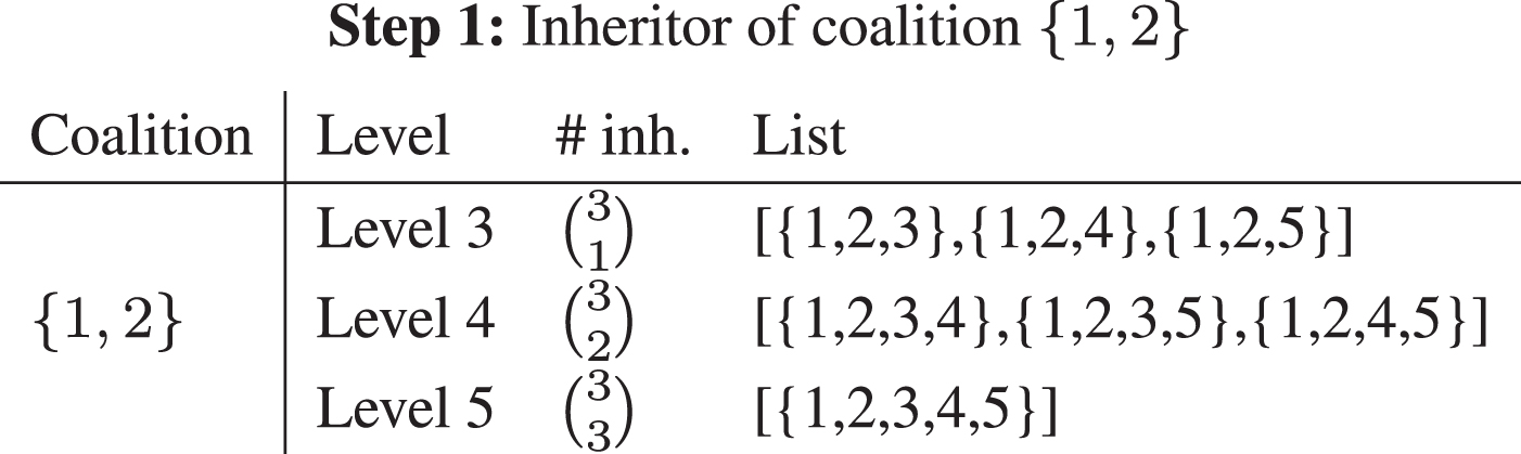
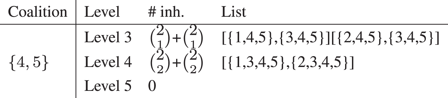
Then, the elements of T which include {1, 2} are duplicated. At the first step there is only one, the whole set N. In the original set, the element 2 is removed while element 1 is removed from its copy. T is updated: T = {{1, 3, 4, 5} , {2, 3, 4, 5}} and this completes the first step. Based on the coefficient order, μ {2, 3} is considered in the second step. Only element {2, 3, 4, 5} may generate inheritors of {2, 3} since {2} is not included in the other element. The summary of this step is given in Table 2.

Table 2

Step 2: Inheritors of coalition {2, 3}

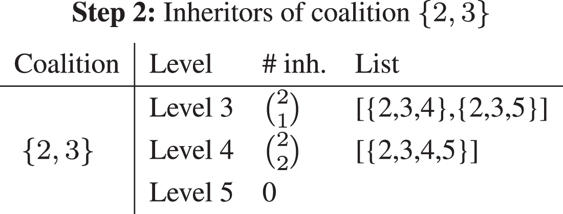
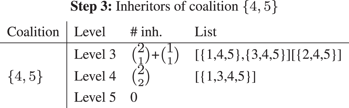
The collection is now updated: {1, 3, 4, 5} remains unchanged, and {2, 3, 4, 5} is replaced by {2, 4, 5} and {3, 4, 5}. As {3, 4, 5} ⊂ {1, 3, 4, 5} it can be removed from the collection to avoid a twofold counting. The collection is now: T = {{1, 3, 4, 5} , {2, 4, 5}}. The next coalition to be considered at the third step is {4, 5}. The results are given in Table 3. T becomes T = {{1, 3, 4} , {1, 3, 5}} as the sets of cardinality k were removed since they cannot generate combinations higher than k.

Table 3

Step 3: Inheritors of coalition {4, 5}

The last step considers the coalition {1, 3}. The results are shown in Table 4.

Table 4

Step 4: Inheritors of coalition {1, 3}

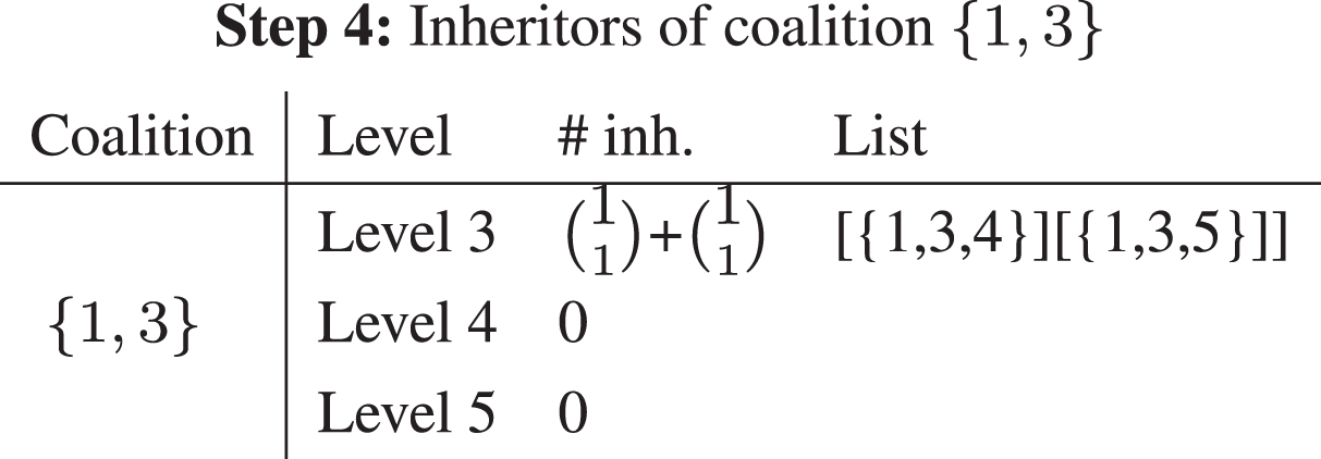
After examining coalition {1, 3} at step 4, 10 coalitions were counted at level 3, 5 at level 4 and 1 at level 5. Consequently, for each level l > k, all coalitions (between brackets) were counted without generating them and the algorithm ends.

If the order of the coefficients were: μ {1, 2}≥ μ {4, 5} ≥ μ {1, 3} …, the result of the second step would be:

In this case {3, 4, 5} would have been counted twice, since its inherits from {1, 3, 4, 5} and {2, 3, 4, 5}. This example shows that a careful counting process is required to avoid this kind of multiple counts, i.e., only distinct sets have to be taken into account.

3.2.3 Counting the number of subsets of p elements included in at least one of subsets of the list

Let S₁, ⋯ , S_m be m subsets of N. Let $\begin{matrix} S_{i} & = & T_{i} \ {{J \ A} \cup {B}}, \\ p & = & l - | {J \ A} \cup {B} | \end{matrix}$ as shown in Algorithm 2. Let $N_{p}^{S_{1}, \dots, S_{m}} = {A \subseteq N : | A | = p and \exists i A \subseteq S_{i}}$ be the set of subsets of p elements of N included in at least one of the subsets S_i, i = 1 ⋯ m. The cardinality of $N_{p}^{S_{1}, \dots, S_{m}}$ is given by the following formula:

$\begin{matrix} | N_{p}^{S_{1}, \dots, S_{m}} | & = & \sum_{i = 1}^{n} (\begin{matrix} | S_{i} | \\ p \end{matrix}) - \sum_{1 \leq i < j \leq m} (\begin{matrix} | S_{i} \cap S_{j} | \\ p \end{matrix}) \\ + \sum_{1 \leq i < j < k \leq m} (\begin{matrix} | S_{i} \cap S_{j} \cap S_{k} | \\ p \end{matrix}) - \dots \\ + (- 1)^{m - 1} (\begin{matrix} | S_{1} \cap \dots \cap S_{m} | \\ p \end{matrix}) \end{matrix}$ (8) with $(\begin{matrix} s \\ p \end{matrix})$ = 0 if p > s. The formula (8) can be written in the condensed form $| N_{p}^{S_{1}, \dots, S_{m}} | = \sum_{k = 1}^{m} (- 1)^{k - 1} A_{k}, where$ (9) $A_{k} = \sum_{1 \leq i_{1} < \dots < i_{k} \leq m} (\begin{matrix} | S_{i_{1}} \cap \dots \cap S_{i_{k}} | \\ p \end{matrix})$ The proof is as follows: $N_{p}^{S_{1}, \dots, S_{m}} = ⋃_{i = 1}^{m} N_{p}^{S_{i}}$ with $N_{p}^{S_{i}} = {A \subseteq N : | A | = p and A \subseteq S_{i}}$ . The principle of inclusion-exclusion [23] states that one has the identity

$\begin{matrix} | ⋃_{i = 1}^{m} N_{p}^{S_{i}} | & = & \sum_{i = 1}^{n} | N_{p}^{S_{i}} | - \sum_{1 \leq i < j \leq m} | N_{p}^{S_{i}} \cap N_{p}^{S_{j}} | \\ + \sum_{1 \leq i < j < k \leq m} | N_{p}^{S_{i}} \cap N_{p}^{S_{j}} \cap N_{p}^{S_{k}} | - \dots \\ + (- 1)^{m - 1} | N_{p}^{S_{1}} \cap \dots \cap N_{p}^{S_{m}} | \end{matrix}$ (10) Notice that $\begin{matrix} N_{p}^{S_{i}} \cap N_{p}^{S_{j}} & = & N_{p}^{S_{i} \cap S_{j}}, \\ N_{p}^{S_{i}} \cap N_{p}^{S_{j}} \cap N_{p}^{S_{k}} & = & N_{p}^{S_{i} \cap S_{j} \cap S_{k}}, \\ \dots \\ N_{p}^{S_{1}} \cap \dots \cap N_{p}^{S_{m}} & = & N_{p}^{S_{1} \cap \dots \cap S_{m}} . \end{matrix}$ Using now the fact that the number of subsets of p elements of a set of s elements is given by $(\begin{matrix} s \\ p \end{matrix}) = \frac{s!}{p! (s - p)!}$ if p ≤ s and $(\begin{matrix} s \\ p \end{matrix})$ = 0 if p > s: $\begin{matrix} | N_{p}^{S_{i}} | & = & (\begin{matrix} | S_{i} | \\ p \end{matrix}), \\ | N_{p}^{S_{i}} \cap N_{p}^{S_{j}} | & = & (\begin{matrix} | S_{i} \cap S_{j} | \\ p \end{matrix}), \\ | N_{p}^{S_{i}} \cap N_{p}^{S_{j}} \cap N_{p}^{S_{k}} | & = & (\begin{matrix} | S_{i} \cap S_{j} \cap S_{k} | \\ p \end{matrix}), \\ \dots \\ | N_{p}^{S_{1}} \cap \dots \cap N_{p}^{S_{m}} | & = & (\begin{matrix} | S_{1} \cap \dots \cap S_{m} | \\ p \end{matrix}) . \end{matrix}$ Replacing in (10) one obtains the formula (8).

4 Complexity analysis

The calculation of gindex according to Eq. (3) is called the standard approach. The two algorithms proposed in this work are referred to as naive and kindex. The computation complexity is analyzed according to space and time considerations. A memory amount of 4 bytes per coefficient is assumed.

The standard approach required 2ⁿ coefficients to be stored in memory and 2ⁿ elements to be summed individually. For n=20, n=25 and n=30 the total memory required is respectively 4Mb, 128Mb and 4Gb. This complexity limits the use of the standard approach to small values of n.

Algorithms naive and kindex take advantage of the underling structure of k-maxitive measures to reduce space or/and time complexity.

For the naive approach, the number of coefficients stored in memory is: $\sum_{i = 1}^{k} (\begin{matrix} n \\ i \end{matrix})$ associated with coalitions up to level k added to elements stored in v, $(\begin{matrix} n \\ k \end{matrix})$ . For instance, if k=4, the total memory required for n=20, n=25 and n=30 is 45Kb, 110Kb and 230Kb, respectively. The naive approach reduces the space requirement and makes the computation tractable for a higher number of elements but does not change the time complexity of the standard approach since all coefficients need to be generated.

For the kindex approach, the number of coefficients stored in memory is: $\sum_{i = 1}^{k} (\begin{matrix} n \\ i \end{matrix})$ + $(\begin{matrix} n \\ k \end{matrix})$ and the size of set |T| which depends on the coefficient values. For k=4, the total memory required for n=20, n=25 and n=30 is approximately 1Mb, 3Mb and 5Mb respectively. These results are the average of a 30 run experiment. In this case, the coefficients of elements up to level k are accessed in the first part of the algorithm (Algorithm 2, Line 3), and then, the coefficients at level k are accessed once more each to complete the second part of the algorithm.

A result summary considering k = 4 for memory usage is shown in Table 6.

Table 5
Step 2^*: Inheritors of coalition {4, 5} for coefficient order μ {1, 2}≥ μ {4, 5} ≥ μ {1, 3} …

Table 6

Memory requirements for the standard, naive and kindex approaches

n	standard	naive	kindex
20	4 MB	45 KB	1 MB
25	128 MB	110 KB	3 MB
30	4 GB	230 KB	5 MB

The number of times the coefficients are read is shown in Table 7.

Table 7

Number of times the coefficients are read for the standard, naive and kindex approaches

n	standard	naive	kindex
20	2²⁰	2²⁰	∼2¹⁴
25	2²⁵	2²⁵	∼2¹⁵
30	2³⁰	2³⁰	∼2¹⁶

The kindex approach demands more space requirement than the naive approach, but it highly reduces the number of individual summations and, consequently, the algorithm running time. Algorithm kindex reduces the access to the coefficient values in 2⁶, 2¹⁰ and 2¹⁴ times compared to the standard and the naive approach.

5 Implementation and application to synthetic data

Some improvements were made to both approaches, many of them dealing with implementations issues. Although these tips do not change the algorithm complexity, they make them faster. The optimized algorithms were then tested using synthetic fuzzy measures to evaluate their performance in different scenarios.

5.1 Optimization enhancements

The alternative formula presented in Eq. (4) to compute the gindex entails a unique summation where all $ℙ (N)$ elements need to be generated. A very efficient way to implement the generation of all subsets of a given set is to use a binary representation. The procedure starts with the decimal number (0) ₁₀ and repeatedly add 1 until (2ⁿ) ₁₀ is reached, while considering their binary representation at each step. When the j^th element is included in the coalition, the j^th bit is set to 1 [5].

The computation of the normalization term in Eq. (3), $\frac{(n - z - a)! \cdot z!}{(n - a + 1)!}$ , and its implementation in kindex (Algorithm 2, Line 14) involves many factorials calculations that would need to be implemented using special data types even for modest values of n. The default data types of most programming languages would produce an overflow if the value is bigger than 20. It can be easily proven that $\frac{(n - z - a)! \cdot z!}{(n - a + 1)!} = \frac{1}{(z + 1) \cdot (\begin{matrix} m \\ t \end{matrix})}$ with m = n - a + 1 and t = n - a - z. The combination $(\begin{matrix} m \\ t \end{matrix})$ can be efficiently solved using an ancient algorithm presented in [6] and shown in the appendix (Algorithm 3). It yields exact results and overflows only for very large n (n larger than 4.10⁹).

The number of elements en each lattice level l is known: $(\begin{matrix} n \\ l \end{matrix})$ . When an element at level k is examined and its inheritors counted, this information can be used to keep track of the number of uncounted elements at each lattice level. When all the elements of a certain level are counted, there is no need to look for inheritors at higher levels, and the loop (Algorithm 2, Line 12) can be interrupted.

When all the inheritors were counted the loop (Algorithm 2, Line 6) can be halted.

When the number of subsets S_{i
_k} in Eq. (8_condensed) increases, the number of combinations to consider might drastically increase the number of calculations. In those cases, it might be better to join all the subsets, consider all possible subsets with increasing cardinality and count those contained in at least one of the S_{i
_k}. A threshold, Thr, can be added to kindex to control which of the two alternatives is used, i.e., if the number of subsets is below the threshold Eq. (8_condensed) is used, otherwise the union is performed. The sensitivity to this parameter is studied in the following section.

5.2 Results

Time performance of kindex and naive kindex are compared for 20 randomly selected subsets belonging to three synthetic randomly generated k-maxitive measures with N = 15, N = 18 and N = 21. Values of k ranging from 2 to 5 and thresholds in the range [4, 20] were evaluated. The results for three typical threshold values are shown in Table 8.

Table 8
Relative time performance of kindex vs naive to compute the gindex value of 20 randomly selected elements of a k-maxitive measure for three threshold values.

Thr=4 Thr=12 Thr=20

N=15 N=18 N=21 N=15 N=18 N=21 N=15 N=18 N=21

k=2 +1.30 +1.25 +2.11 +2.35 +2.11 +3.88 +1.81 -1.70 +3.54

k=3 +3.80 +3.60 +2.18 +4.21 +4.09 +2.28 +1.63 -1.46 +1.96

k=4 +4.24 +6.40 +8.60 +4.25 +6.54 +8.79 +3.45 +1.17 +3.01

k=5 +2.82 +5.49 +6.77 +2.78 +5.52 +6.80 +2.44 +1.45 +4.50

AVG +3.04 +4.19 +4.92 +3.40 +4.57 +5.44 +2.33 -0.17 +3.25

	Thr=4	Thr=12	Thr=20
k=2	+1.30	+1.25	+2.11	+2.35	+2.11	+3.88	+1.81	-1.70	+3.54
k=3	+3.80	+3.60	+2.18	+4.21	+4.09	+2.28	+1.63	-1.46	+1.96
k=4	+4.24	+6.40	+8.60	+4.25	+6.54	+8.79	+3.45	+1.17	+3.01
k=5	+2.82	+5.49	+6.77	+2.78	+5.52	+6.80	+2.44	+1.45	+4.50
AVG	+3.04	+4.19	+4.92	+3.40	+4.57	+5.44	+2.33	-0.17	+3.25

The highest value, +8.79, indicates that kindex is almost 9 times faster than the naive approach when N=21, k=4 and Thr=12. In fact, kindex outperforms naive kindex in almost all tested scenarios, except for Thr=20, k=2 and k=3. An average of the last row on each threshold shows that kindex is 1.8 better than naive in the worst case (for Thr=20) and 4.47 better in the best case (for Thr=12). The best performance, in average (in boldface), is obtained for Thr=12. In all the scenarios, kindex performance increases (on average) with the number of features considered, i.e., the higher the N the better its performance compare to the naive approach. The fact that the difference between performances increases with the number of elements is expected since the number of subsets that do not need to be generated by kindex grows with the number of elements in N.

A combination of a big threshold and a small N (N=15 and Thr=20) makes the algorithm kindex use Eq. (8_condensed) most of the time. In the other case, for a combination of a small threshold and a big N (N=21 and Thr=4), the approach of join all the subsets is used most of the times. A balance is obtained when considering a threshold around N/2.

A reasonable strategy, to significantly reduce time requirement, is to start computing the gindex of singletons. Then, for the gindex of coefficients pairs, consider only the coalitions of relevant singletons (gindex ≥ 1/n) [15]. This strategy can be repeated, in an analogous way for higher size subsets. Moreover, to speed up the process, the computation of the elements can be performed in a parallel way.

6 Conclusions

In this work, two algorithms, called naive kindex and kindex, are proposed. They compute the gindex from a k-maxitive measure where only coefficients up to k are stored in memory. In naive kindex, each subset is efficiently generated thanks to a binary representation, and the computation of the maximum in Eq. (6) is optimized by ordering coalitions of level k at the beginning of the algorithm. The kindex approach is divided into two parts. In the first part, the contribution of elements up to level k to the gindex (A) is done by using naive kindex. In the second part, gindex is computed considering the contribution of each k level element together with the contributions of its inheritors. In this way, the generation of higher order set is avoided and the time complexity of the algorithm is considerably reduced.

Optimization enhancements are suggested for both approaches: generation of subsets, computation of combinatorial numbers, halting criteria for loops and selection of a threshold to decide whether to use or not Eq. (8_condensed) to count subsets of a specific cardinality.

Both algorithms significantly reduce the space requirement compared to the standard approach. For kindex, the number of calls is reduced, since all inheritors of the same element are collectively computed. The price to pay is a small amount of extra memory space to avoid counting an element more than once (vector v).

The time performance of the two proposed approaches is tested for synthetic k-maxitive fuzzy measures. kindex is faster and the difference is more significant when more elements are considered. When analyzing a fuzzy measure, the processing time can be reduced by restricting the analysis to coalitions of interest. First, only small size coalitions, e.g., up to k + 1 elements, can be considered since the use of a k-maxitive measure assumes that the interactions involve at most k elements. But, among these coalitions only those including relevant singletons have to be studied. A singleton is said to be relevant if its gindex value is higher than 1/n as discussed in [15].

One optimization issue is left as a perspective of this work: a parallel version of the kindex algorithm to compute the gindex for different coalitions as each computation is independent from others even if it is based on the same information.

Footnotes

Appendix

A. An algorithm that efficiently computes $(\begin{matrix} n \\ t \end{matrix})$

Algorithm Choose (Algorithm 3) shows an efficient way to compute the combination of n elements taken t at the time [6].

Algorithm 3 Choose

1: Input: n: total number of elements; t: number of taken elements.

2: Output: $(\begin{matrix} n \\ t \end{matrix})$

3: r ← 1

4: d ← 1

5: while d ≤ t do

6: r ← r.n

7: n ← n –1

8: r ← r/d

9: d ← d + 1

10: end while

References

Beliakov

and Wu

J.-Z.

, Learning fuzzy measures from data: Simplifications and optimisation strategies, Information Sciences 494 (2019), 100–113.

Calvo

and de Baets

, Aggregation Operators Defined by k-Order Additive/Maxitive Fuzzy Measures, International Journal of Uncertainty, Fuzziness and Knowledge-Based Systems (06) (1998), 533–550.

Grabisch

, k-order additive discrete fuzzy measures and their representation, Fuzzy Sets and Systems 2 (1997), 167–189.

Grabisch

, Fuzzy Measures and Integrals: Recent Developments, Springer International Publishing, Cham, 2015, 125–151.

Knuth

, The Art of Computer Programming: Combinatorial Algorithms, Part 1, Addison-Wesley Professional, 2011.

Knuth

, The Art of Computer Programming, Volume 2: Seminumerical Algorithms, Addison-Wesley Longman Publishing Co., 1997.

Kochi

and Wang

, An algebraic method and a genetic algorithm to the identification of fuzzy measures based on choquet integrals, Journal of Intelligent & Fuzzy Systems: Applications in Engineering and Technology 26 (2014), 1393–1400.

Maafa

, Nourine

and Radjef

M. S.

, Algorithms for computing the shapley value of cooperative games on lattices, Discrete Applied Mathematics, 2018.

Magoč

, Modave

, Ceberio

and Kreinovich

, Computational methods for investment portfolio: The use of fuzzy measures and constraint programming for risk management, Foundations of Computational Intelligence 2 (2009), 133–173.

10.

Marichal

J.-L.

and Roubens

, Determination of weights of interacting criteria from a reference set, European Journal of Operational Research (3) (2000), 641–650.

11.

Mesiar

, Generalizations of k-order additive discrete fuzzy measures, Fuzzy Sets and Systems (3) (1999), 423–428.

12.

Mesiar

, k-order additive fuzzy measures, International Journal of Uncertainty, Fuzziness and Knowledge-Based Systems 6 (1999), 561–568.

13.

Murillo

, Guillaume

, Tapia

and Bulacio

, Revised hlms: A useful algorithm for fuzzy measure identification, Information Fusion (4) (2013), 532–540.

14.

Murillo

, Guillaume

and Bulacio

, k-maxitive fuzzy measures: A scalable approach to model interactions, Fuzzy Sets and Systems (2017), 33–48.

15.

Murillo

, Guillaume

, Spetale

, Tapia

and Bulacio

, Set characterization-selection towards classification based on interaction index, Fuzzy Sets and Systems (2015), 74–89.

16.

Murofushi

and Soneda

, Techniques for reading fuzzy measures (iii): interaction index, in: 9th Fuzzy System Symposium (1993), 693–696.

17.

Popescu

and Keller

, Fuzzy measures on the gene ontology for geneproduct similarity, IEEE/ACM transactions on computational biology and bioinformatics/IEEE (2006), 263–274.

18.

Rodríguez-Veiga

, Novoa-Flores

and Casas-Méndez

, Implementing generating functions to obtain power indices with coalition configuration, Discrete Applied Mathematics, (2016), 1–15.

19.

Shapley

, A value for n-person games, in: H. Kuhn, A. Tucker (Eds.), Contributions to the Theory of Games, vol II, Vol. 28 of Annals ofMathematics Studies, (1953), 307–317.

20.

Sugeno

, Theory of fuzzy integrals and its applications, Ph.D. thesis, Tokyo Institute of Technology, (1974).

21.

Sugeno

and Terano

, A model of learning based on fuzzy information, Kybernetes 6 (1977), 157–166.

22.

Únver

, Ózcelik

and Olgun

, A fuzzy measure theoretical approach for multi criteria decision making problems containing sub-criteria, Journal of Intelligent & Fuzzy Systems 35 (2018), 1–8.

23.

Van Lint

and Wilson

, A Course in Combinatorics, Cambridge University Press, 2001.

24.

Wang

, Leung

and Wang

, A genetic algorithm for determining non-additive set functions in information fusion, Fuzzy Sets and Systems 102 (1999), 436–469.

25.

J.-Z.

, Yu

L.-P.

, Li

, Jin

and Du

, The sum interaction indices of some particular families of monotone measures, Journal of Intelligent & Fuzzy Systems 31 (2016), 1447–1457.

26.

J.-Z.

, Yu

L.-P.

, Li

, Jin

and Du

, Using the monotone measure sum to enrich the measurement of the interaction of multiple decision criteria, Journal of Intelligent & Fuzzy Systems 30, 2015.

27.

Yager

and Alajlan

, Fuzzy measures in multi-criteria decision making, in: Procedia Computer Science: Proceedings of the 2015 International Conference on Soft Computing and Software Engineering 62 (2015), 107–115.

28.

Zhang

and Zhang

, Fuzzy measures and granular computing, in: Rough Set andKnowledge Technology, in Proceedings of the 5th International Conference, (2010), 759–765.

An algorithm for computing the generalized interaction index for k -maxitive fuzzy measures

Abstract

Keywords

1 Introduction

2 Preliminaries

2.1 Fuzzy measures and their representation

3.1 First approach: a naive implementation

3.2.1 gindex algorithm for k-maxitive fuzzy measures: kindex algorithm

3.2.2 Method to avoid counting associated inheritors more than once

Table 1 Step 1: Inheritor of coalition {1, 2}

Table 5 Step 2*: Inheritors of coalition {4, 5} for coefficient order μ {1, 2}≥ μ {4, 5} ≥ μ {1, 3} …

5.1 Optimization enhancements

5.2 Results

Footnotes

Appendix

References

Table 1
Step 1: Inheritor of coalition {1, 2}

Table 5
Step 2^*: Inheritors of coalition {4, 5} for coefficient order μ {1, 2}≥ μ {4, 5} ≥ μ {1, 3} …