
Abstract
With the wide application of attention mechanism in multitudinous field of natural language processing (NLP), to date various deep neural networks based on this mechanism have been introduced and developed. However, a major problem with this kind of application is that a long time will be consumed due to the current networks still need to rely on their own ability to form attention values from scratch during the training. In this paper, we propose an auxiliary method called the Guided Attention Mechanism (GAM), which utilizes the prior knowledge to guide the network to form attention values in NLP field, thereby shortening the network training time and making the attention values more accurate. This work designed two sets of prior knowledge generation processes based on the regularization method and the deep learning method respectively. And the prior knowledge is used to guide the attention values of the original network in terms of values and angles. The experimental results show that compared with the original network, the classification accuracy of the network using GAM is improved by about 2%, and the training time is reduced by 5∼9%.
Introduction
Deep neural networks have achieved tremendous success in image fields such as target classification [1], object detection [2], etc. When introducing them into various natural language processing (NLP) tasks, researchers found that, unlike the independence of pixels, words have a significant sequential relationship in the text. The combination of words in different orders causes the text to present different semantics, which makes the fully connected neural network no longer suitable for text processing. To overcome this problem, early NLP tasks mainly relied on recurrent neural networks (RNNs) [3], RNNs learned the positional relationship between inputs through a cyclic structure and is applied to many fields such as classification of brain signals [4], Takagi-Sugeno fuzzy models [5] etc. However, with the increase of text length, more redundant information is brought into the network, which also leads to the issues of gradient disappearance and gradient explosion. After that, two complex structures, Long Short-Term Memory (LSTM) [6] and Gated Rectified Unit (GRU) [7], were applied to the RNNs. They achieve the effect of selecting and filtering information by adding some gate structures to the RNN’s recurrent unit. In addition to using more complex network structures, the embedded representation of words has also been widely used and studied. Its idea is to train a special deep learning network [8, 9] by using a large amount of corpus to make words that are close in meaning appear closer in the embedded space, and thus providing some semantic knowledge to accelerate the network’s understanding of the input text. Although this method can reflect the semantic relationship between words, it cannot show the influence of different words on the text.
As the scene becomes more diverse, the description of the text becomes more complicated. Researchers endeavor to make models automatically focus on the words that have decisive effect and capture the important semantic information in a sentence, which led to the widespread use of attention mechanism. The purpose of this mechanism is to calculate a set of weights for the input text to indicate the importance of words in the corresponding position. The initial attention mechanism was based on RNNs, which was first applied to machine translation [10] and achieved the best results at that time. After this, lots of NLP tasks, such as question answer [11], text classification [12], Aspect-level sentiment classification [13], began to combine attention mechanism in the construction of the model, and achieved significant breakthroughs in effect. However, restricted by the recurrent structure of the RNN, the input information is hard to get parallel processing in the network. So that the attention value of the current moment cannot be calculated until the output of the previous moment is generated, which increases the time for network forward propagation and training. At present, convolutional attention mechanism [14] and self-attention mechanism [15] have been proposed to improve this problem. The former uses a convolutional network to extract features and calculate attention values, while the latter directly compares words at different locations of the input text to obtain attention values. Among them, BERT [16] and GPT [17], which are based on the self-attention mechanism, can advance the state of the art for many NLP tasks.
By changing and adjusting the structure of the attention mechanism, the network can be given stronger performance. But, during training, one of the main obstacles is that the attention networks need to rely on their own ability to form the attention values from scratch which increases the difficulty of learning. To this end, some methods in the image field attempt to introduce prior knowledge to generate attention values for input data. For example, using the image to guide the attention values of the text [18], the audio information is utilized to guide the attention values of the image [19], and the image and the attribute mutually guide the attention values [20].
In our paper, guided attention mechanism (GAM), a general method of guiding attention in NLP field, is proposed to speed up the formation of networks’ attention values and improve their accuracy. As shown in Fig. 1, unlike that the prior knowledge in [18–20] is independent of the input data and used directly to generate the attention values. GAM will first calculate a set of guiding values(GVs)(which is priori knowledge) for each text. Then, by using some mathematical methods, the attention values of the taught network will generate new attention values with the help of GVs, there the taught network refers to any network which generates attention values for input data. Finally, the new attention values will replace the old one and be guided by GVs again in the next iteration.
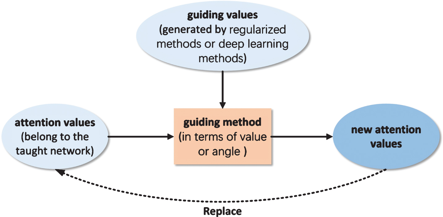
The process framework of GAM.
In summary, our contributions are three-fold: A set of process, which based on a new text categorization network designed by us, is utilized to generate GVs was proposed. And a regularized process, which based on a public emotional dictionary, was described. We applied some preprocessing operations on the public emotional dictionary to obtain GVs. In the experiment, the two sets of processes were compared. The advantages and disadvantages of the two processes and their application scenarios were also emphasized; Two methods for using GVs to guide attention values were designed. One of them combines some widely used activation functions. The other applies the new loss function we defined; We present a complete and general process for guiding attention values in the NLP field and verify the effectiveness of GAM on six tasks.
The remainder of the paper is shown as follows. In Section 2, the related work is discussed. Section 3 introduces two processes for generating GVs, and each step is described in detail. In Section 4, two methods for guiding the attention values of the taught network based on the GVs are provided, and the basic ideas of each method are illustrated mathematically. The datasets used in the experiments and the parameters of the experimental models are listed in Section 5. The experimental results are discussed and analyzed in Section 6. In Section 7, the paper is discussed and concluded.
In most kinds of NLP tasks, to obtain the important semantic information, the network is expected to have a focus when learning text, which is often referred to as attention. When the input sentence is x and the target output is y, the forward propagation process of the model with attention mechanism can be abbreviated as formula (1), where g (x) is the attention values calculated for input x:
At present, considerable research have been devoted to design g (·). According to the structure of the network, the existing attention mechanisms can be divided into recurrent attention mechanism (RAM) [10], convolutional attention mechanism (CAM) [14] and self-attention mechanism (SAM) [15]. There three attention mechanisms change the optimization objective of the model from maximizing conditional probability p (y|x) to p (y|c). Where c is the context vector, which can be expressed as c = z (x, g (x)). Among them, RAM and SAM are widely used in many NLP tasks [21].
The main feature of RAM is based on RNN, and it is necessary to continuously calculate the attention value during the cycle. Taking machine translation as an example, its structure is shown in Fig. 2(a).

Two attention mechanisms.
The input vectors x1, x2, …, x T x generate annotation sequencesh1, h2, …, h T x through a layer of bidirectional RNN. Each annotation h i contains information about the whole input sequence with a strong focus on the parts surrounding the i th word of the input sequence. The context vector c i is computed as a weighted sum of annotations h i in formula (2):
α ij is the attention value corresponding to the annotation h j at time i, and its calculation is formula (3), Where F (·) is a fully connected network with an output node of 1, which uses w α and b α as weights and bias.
RAM assigns a weight value to the output information of each moment. These weight values are constantly adjusted during the back propagation to make the model gradually pay attention. Due to the good performance of this mechanism, many NLP fields have been developed by leaps and bounds. In machine translation [10], encoding the source sentence into a fixed-length vector becomes the bottleneck of the encoder-decoder architecture. The phrase-based translation system built by incorporating the attention mechanism is superior to all the networks at that time. In question answering [22], using simple entity detection and anonymisation algorithms to construct datasets and combining attention mechanisms allows the model to answer complex questions with minimal prior knowledge of language structure. In order to enable the model to learn the hierarchical structure of the document, the hierarchical attention network [23], which applied the attention mechanism at both the word and sentence levels, was proposed. Experiments show that this method is significantly better than the previous method in document classification.
Restricted by the physical structure of the model, RAM cannot input data in parallel, which leads to longer training time, even if optimization schemes such as factorization tricks [24] and conditional computation [25] can improve computational performance, but this limitation still exists. SAM was proposed to solve this problem.
SAM correlates information from different locations on the input sequence as a representation. Its structure is shown in Fig. 2(b). The entire operation can be expressed as:
Inputs include queries (Q) and keys (K) with dimension d
k
, and values (V) with dimension d
v
. By calculating queries and keys, the attention value corresponding to values is obtained as
SAM avoids the additional cost of cyclic input by feeding the information into the network at one time. This mechanism also contributes to some new network structures including Transformer [15]. The BERT [16] network based on the multi-layer Transformer overcomes the long-term dependence problem caused by long text and has been proven to obtain new state-of-the-art results on eleven NLP fields. In the learning task, a large amount of unlabeled corpus with abundant information cannot be used in model training, this limitation is effectively solved by combining unsupervised learning with GPT [17] built on Transformer.
The above two attention mechanisms can give the model better performance by mean of different calculation methods. However, in the initial iteration of the model, due to the randomness of each hyperparameter, the attention direction changes constantly, which makes the convergence speed of the model is slower. In order to solve this problem and shorten the training time of the model, this paper proposes the Guided Attention Mechanism (GAM), which provides accurate directional guidance for the model, and ensures that attention values can be adjusted according to actual data.
Currently, in NLP field, the research on adding prior knowledge before network training mostly focuses on the vectorized representation of words [26, 27], but too little work has been devoted to provide prior knowledge for network to help it form attention values. In this section, we describe two sets of processes for generating guiding values (GVs). They will use regularized methods (Sec. 3.1) and deep learning methods (Sec. 3.2) respectively to generate GVs (i.e. prior knowledge) for each text input into the network, whose effects are shown in Fig. 3(a) and Fig. 3(b) (The darker the color, the larger the corresponding value).
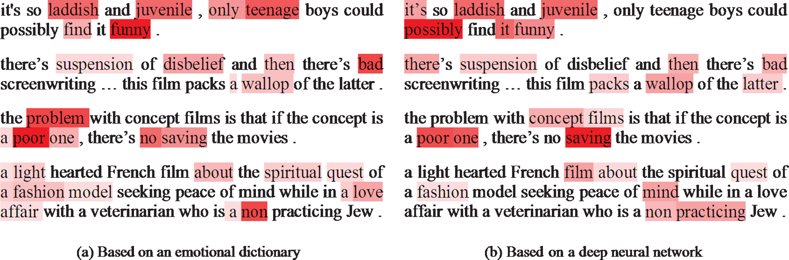
Visual representation of the guiding values.
GVs generated by the two processes need to show the taught network which areas of the text it should focus on, without being detailed to every word. So as to ensure the fault-tolerance and independent learning ability of the taught network.
When reading an article, people’s eyes are often attracted by words or short sentences with rich potential meanings. But they will not pay too much attention to adverbs, prepositions and some words which are insipid or just used to conform to grammatical norms. These potential meanings include, but are not limited to, the author’s emotional richness, subjective consciousness, and the foreshadowing of the following text. Considering the use of existing means to numerically describe the subjective consciousness and the author’s foreshadowing of the following text is very difficult. In our experiment, the emotional richness of the words is used as an auxiliary tool of the regularization method to simulate human reading behavior.
SentiWordNet [28], an emotional dictionary published by opinion mining, has a wide coverage and a high degree of detail. For example, the word ‘good’ is listed 4 meanings as nouns in the dictionary, 21 meanings as adjectives and 2 meanings as adverbs, and three scores for each meaning: positivity, negativity, objectivity.
In this study, SentiWordNet3.0 [29], the latest edition of this series of emotional dictionaries, was selected. Each word in the dictionary is pre-processed to calculate the corresponding average emotional score, which is used to express the emotional richness of the word, such as formula (5):
Where n is the number of meanings of a word in the dictionary, pos _ score i and neg _ score i is the positive and negative scores marked by the dictionary in the i th meaning.
As expressed in the formula (6), the text is traversed first, and if the words are included in the dictionary, the corresponding emotional score is taken, otherwise it is taken as 0. After the replacement is completed, all the values are normalized to obtain GVs g1, g2, …, g
Tx
.
Part of the effect of this method is shown in Fig. 3(a). It can be found that not only adjectives but also some nouns and verbs in sentences have high emotional score, which also proves the usability and generalization of SentiWordNet3.0.
The main advantage of using emotional dictionary to generate GVs is that it has low computational complexity and fast computational speed. However, limited by the size of emotional dictionary, words that contain rich emotions but do not appear in the dictionary will not be able to give the corresponding emotional score. At the same time, the emotional score of the same word in different sentences will not be different owing to this method does not combine the semantics of sentences. Therefore, the longer the length of the input text, the more words it contains, the better the effect.
Different from the regularized method, the main idea of this section is to train a new classification model and use it to generate a corresponding emotional value for each word in the text, and then calculate GVs based on these emotional values. The model used to generate the emotional values is referred to as the guiding network in this paper, and its structure is shown in Fig. 4.
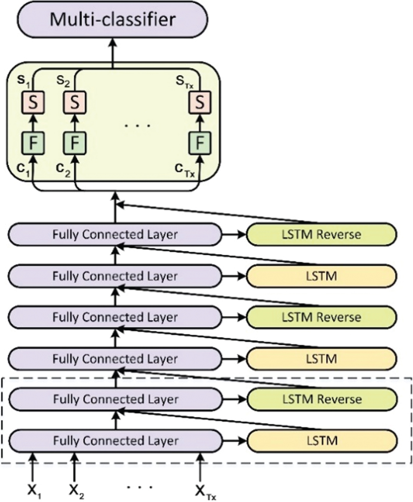
Guiding network.
Before training the guiding network, we select the Yelp reviews full star dataset [30] as the training corpus which is constructed by randomly taking 130000 training samples and 10000 testing sample for each review star from 1 to 5. And each word in samples is initialized to be a 100 × 1 dimensional vector x by Glove100 [9]. The values in the weight and bias matrix used in the forward propagation are initialized by randomly sampling from uniform distribution in [- 1, 1].
In forward propagation, the input x1, x2, …, x
Tx
∈ R100×Tx, first pass into a fully connected layer and an LSTM layer, their outputs then become inputs to another fully connected layer and reverse LSTM layer. Here, the forward LSTM and reverse LSTM are not input at the same time and their input tensors are different. Therefore, this structure shown by the dashed box in Fig. 4 is called asynchronous bidirectional LSTM layer where LSTM with long-term memory and selective forgetting ability is chosen to extract deep features of text. Since the input to each layer contains the output of a fully connected layer, more original information can be retained than the existing bidirectional LSTM layer. Referring to the experimental results in [31] on the selection of the number of LSTM output nodes. The number of output nodes of the forward LSTM layer, the reverse LSTM layer, and the fully connected layer in this structure is set to 100. The calculation of asynchronous bidirectional LSTM layer is as shown in formula (7), where w1 ∈ R100×100 and w2 ∈ R200×100 are weight matrices in two fully connected layers, b1 ∈ RTx×100 and b2 ∈ RTx×100 are bias matrix, l41, l42, …, l4Tx ∈ R200×Tx represents the final output of this structure. The relationship between the reverse LSTM layer and the forward LSTM layer can be expressed as LSTM _ Reverse (l31, l32, …, l3Tx) = LSTM (l3Tx, …, l32, l31).
Considering the limited ability of single-layer asynchronous bidirectional LSTM, a 3-layer stack structure (where the dimension of the weight w1 in the last two layers is changed to 200 × 100) is adopted in the guiding network to extract deep semantic feature c1, c2, …, c
Tx
∈ R200×Tx. Then, the values at each position of c1, c2, …, c
Tx
are respectively taken into a forward fully connected layer F and a sigmoid (·) activation layer S. As shown in formula (8), where c
i
∈ R200×1 is the input of the current position, w
fi
∈ R200×1 and b
fi
∈ R1×1 respectively represent the weight and bias in the F layer. The weight of each F layer will not be shared, and finally the output s1, s2, …, s
Tx
∈ R1×Tx whose values are between (0, 1) are obtained.
We call s1, s2, …, s
Tx
the emotional values extracted from x1, x2, …, x
Tx
. Subsequently, s1, s2, …, s
Tx
are sent as input information to a multi-classifier. The multi-classifier is operated as follows:
Where class _ number represents the number of categories of the classification,w c ∈ RTx×class_number is the weight matrix and b c ∈ R1×class_number is the bias matrix, p1, p2, …, pclass_number ∈ R1×class_number is the final output of the guiding network.
We divide texts into two categories based on whether they have significant emotional tendency and use them to train the network. Texts with obvious emotional tendencies often contain some words with rich emotions, which play a crucial role in the final decision of the network. As the classification accuracy of the two types of texts continues to increase, network will gradually have an ability to distinguish between emotionally rich words and other words. When the text is input into the trained network, the value between the corresponding s1, s2, …, s Tx will fluctuate due to the difference in the degree of emotional richness between words. There are great fluctuations between words with rich emotions and other words. GVs will be based on these fluctuations.
Samples labeled as 1 and 5 stars in the Yelp data set are grouped into texts with significant sentimental tendencies, and the remaining samples are grouped into another class. class _ number is 2. The cross entropy error function is chosen as the loss function, the batch size is set to 32, the network optimizer selects AdamOptimier.
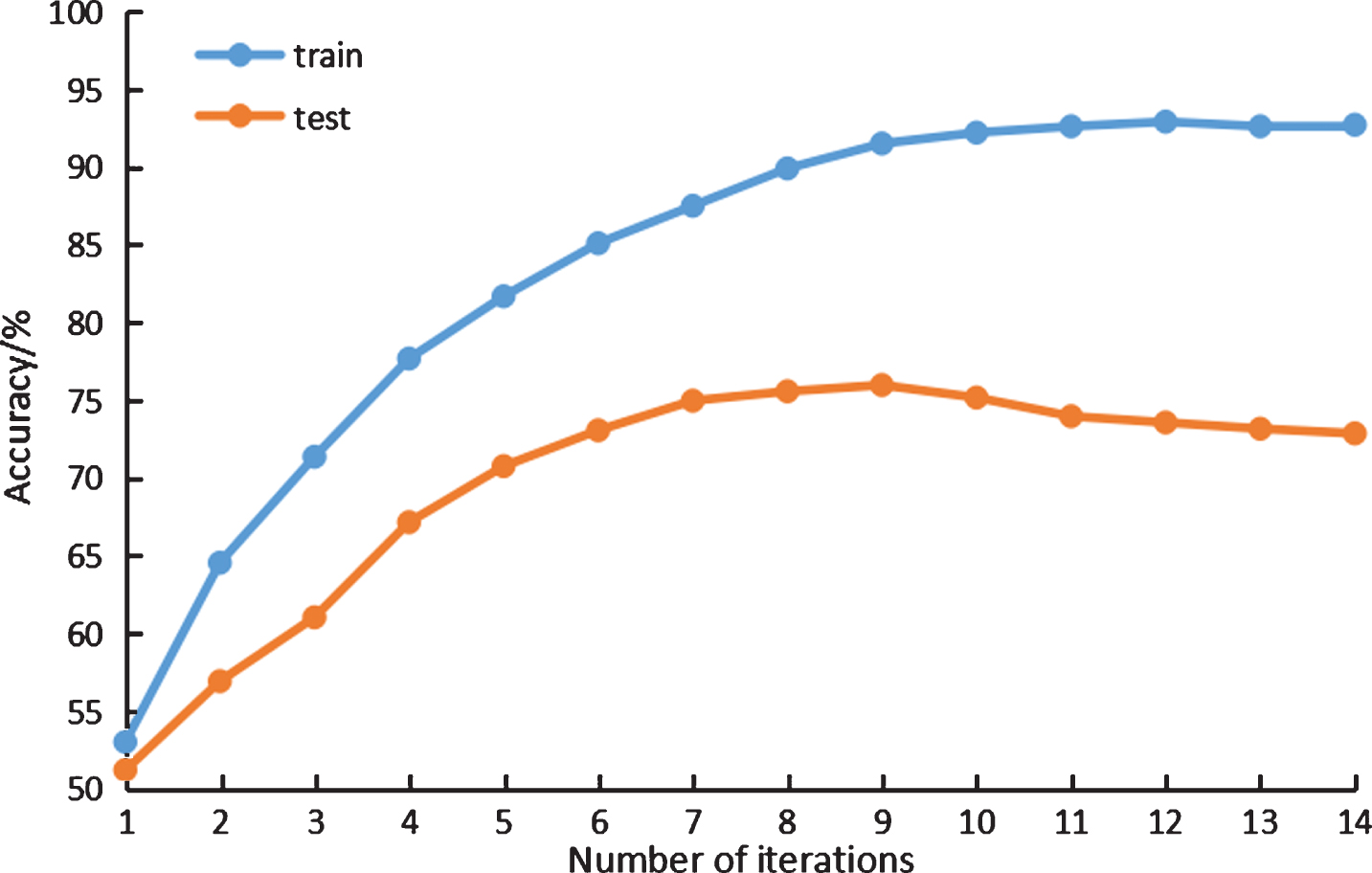
We randomly select 80% of each class of text to form the training dataset, and the rest data to form the test dataset. Each word in the text will be initialized to a word vector by using Glove100. Subsequently, the training data is fed into the guiding network for iterative training, and the test data is fed into the network to test the model performance after each iteration. The accuracy of the network in training data and test data varies with the number of iterations as shown in Fig. 5. It can be seen from Fig. 5 that the model achieves the highest accuracy of 76.2% on the test data after the 9th iteration, and then the accuracy decreases due to overfitting. Therefore, the training is ended after the completion of the 9th iteration.
Accuracy varies with the number of iterations.
When the training is complete, we will feed the text that needs to generate GVs into the network and take out the corresponding s1, s2, …, s Tx . As shown in formula (11), s1, s2, …, s Tx are input to the function maxN (·).maxN (s1, s2, …, s Tx ) first subtracts item by item and takes their absolute values to generate |s Tx - s1|, |s1 - s2|, …, |sTx-1 - s Tx |, which is used to quantify the magnitude of the fluctuation. Then, selecting the items with the top N largest values in the |s Tx - s1|, |s1 - s2|, …, |sTx-1 - s Tx | (N depends on the length of sequence) and return the values on the right side of the minus sign in these N items. These N values will form a new sequence as the output of max _ N (s1, s2, …, s Tx ), if s i exists in this sequence, it is retained, otherwise it is set to 0. Finally, the sequence is normalized to get g1, g2, …, g Tx which is GVs. Part of the effect of this method is shown in Fig. 3(b).
The main advantage of the guiding network is that it owns good generalization. For each input text, GVs can be generated according to its semantics. However, in order to ensure that the network has good feature extraction capabilities, a large amount of training corpus is needed. And due to the complicated structure, the time for processing a single sentence is longer than using an emotional dictionary. Therefore, this method is more suitable for the case where the length of input text is shorter, and for the long text, the training data may need to be re-selected for the network.
In forward propagation, almost all networks that use the attention mechanism will calculate one or more sets of weight values t1, t2, …, t Tx for the input sequence. By normalizing these weights, the attention values α1, α2, …, α Tx are obtained, and they are constantly adjusted during the back propagation. Based on the guiding values g1, g2, …, g Tx mentioned in Section 3, we designed the method of guiding attention in terms of value (Sec. 4.1) and angle (Sec. 4.2), which aims to make the taught network quickly form attention after being guided by GVs.
Guide the values
The flow of the method of guiding the numerical value is shown in Fig. 6, and the mathematical description is as follows:
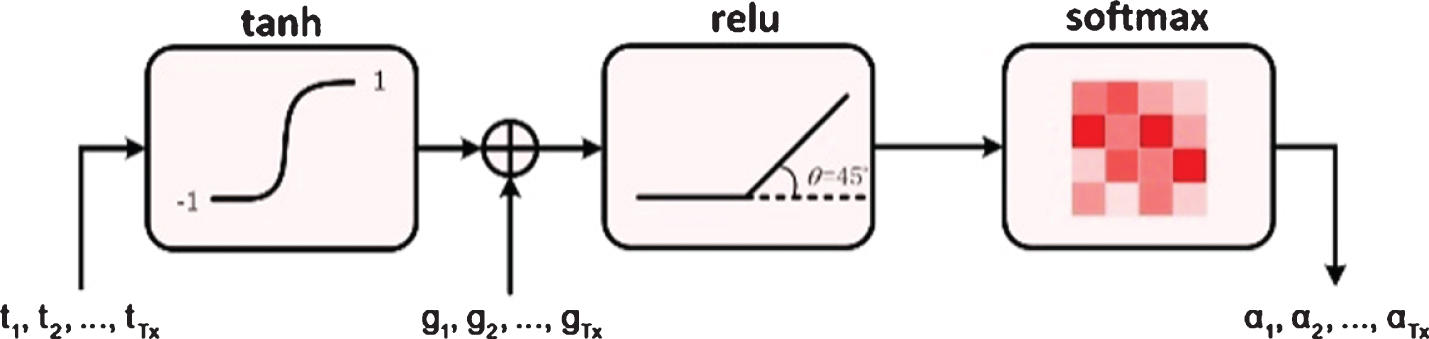
Method of guiding numerical values.
The weight values t1, t2, …, t
Tx
∈ (- ∞ , + ∞) calculated by the taught network convert the range of values to (- 1, 1) through the tanh(·) function. While g1, g2, …, g
Tx
∈ (0, 1), summing the two sequences yields h1, h2, …, h
Tx
. These operations can serve the following two purposes: The final attention values of the taught network will be based on GVs, and GVs will exert influence throughout the learning process; Where the GVs is wrong, the taught network can weaken its influence by adding negative values. And for those areas that GVs have not noticed, the taught network can also concern them by adding positive values.
The negative values in h1, h2, …, h Tx are the part that the taught network is unwilling to care about or is overcorrected. This part should not be taken into account when calculating the final attention values. So relu (·) function is chosen to take the negative values to zero, and then the final attention values α1, α2, …, α Tx are obtained by normalizing the sequence with softmax(·) function.
From the above calculation process, it shows that the attention values formed by the taught network are the result of modifying and perfecting GVs, which avoids the need to adjust the attention values by a large margin. In the whole process of guidance, no additional parameters are introduced, only some non-linear activation functions are used to transform the values, so there is no additional time consumption.
Vectors of any dimension can be represented in a specific vector space, the guiding values g1, g2, …, g Tx and the attention values α1, α2, …, α Tx of the taught network in the vector space as shown in Fig. 7(a).
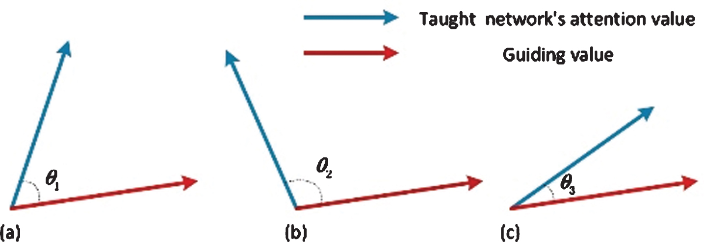
Spatial representation of the vector.
In vector space, the cosine value of angle θ is used to measure the difference between two vectors. It is expressed as formula (13)
When the two vectors are not similar, cos θ tends to 0, the larger the θ is. As shown in Fig. 7(b), the two vectors appear more separated in space. When the two vectors are more similar, cos θ tends to 1, and smaller the θ is, as shown in Fig. 7(c), the two vectors appear closer in space.
In the process of guiding, we hope that the attention values of the taught network can be quickly approached to the GVs, and maintain a certain angle between the two to ensure the independence of the taught network. This requires that cos θ can be increased to a limited extent during training. For this reason, the loss function of the network is revised as formula (14).
The new loss function adds ω (1 - cosθ) to the original, where ω ∈ [0, + ∞) is the penalty coefficient, which is a constant.
In order to minimize the loss function, the taught network will reduce the value of the (1 - cosθ) when optimizing the hyperparameters, which will lead to the increase of cos θ. In space, it shows that the attention vector of the taught network is close to the GVs vector. By adjusting the penalty coefficient ω, the over-fitting between the two vectors can be prevented. When ω increases, the value of the ω (1 - cosθ) becomes larger which causes the network imposes more punishments on (1 - cosθ) to make its value smaller. However, when ω decreases, the value of ω (1 - cosθ) becomes smaller, the network will weaken the penalty for the (1 - cosθ) to make its value larger. After several attempts, we recommend setting the value of ω to [0.001, 0.01].
The method of guiding the angle quickly forms attention values by narrowing the angle between the two vectors. The difference from the method in section 4.1 is that the method of this section is intended to make the attention values of the taught network close to GVs, rather than modifying it. By adding penalty coefficient ω, The size of the angle between two vectors becomes controllable.
To verify the effectiveness and generalization of GAM, six public datasets were selected in this experiment, and the classification task was performed on them.
Datasets
The following six public datasets were selected for comparison experiments. The information of each dataset is shown in Table 1. Columns 5 and 6 of the table represent the number of words contained in the datasets and the value of N (mentioned in Section 3.2) chosen for the datasets. In this experiment, Glove100 [9] trained by Wikipedia data was used to initialize the word vector of each word. In order to reduce the contingency in the experiment, each dataset was tested by a five-fold cross validation method.
Distribution of each dataset
Distribution of each dataset
To confirm the validity and generalization of GAM, we selected a widely used and representative network from recurrent attention mechanism and self-attention mechanism respectively. The recurrent attention mechanism corresponds to the bidirectional LSTM combined with the attention mechanism (Bilstm+attention) [10], and the self-attention mechanism corresponds to the Transformer [15]. The structure of each network is consistent with that in original literature, the hidden units of all LSTM is 300, the word vector dimension of each word is 100 and they are fine-tuned during training to improve the performance of classification.
Before the experiment, we generated GVs for the six datasets based on the two sets of processes described in Section 3. Using dga and lga to represent GVs generated by using emotional dictionary and deep learning network respectively. The two selected networks will use the two types of GVs and two guiding methods proposed in Section 4. The two guiding methods are abbreviated as VG (Section 4.1) and AG (Section 4.2), respectively. As will be described below, for example, Transformer_VG_dga will be used to abbreviate a network that combines GVs. Except for structural inconsistency, other parameters of each network are consistent during training. The batch size is set to 32, the network optimizer selects AdamOptimier, and the penalty coefficient ω is set to 0.008. During the experiment, the same training procedures and the same dataset are applied for all networks.
Results
The performance of the eight new networks using the GAM and the original networks on the six datasets is shown in Table 2. Meanwhile, some high-performance networks and methods, and their corresponding classification accuracy is also listed.
Performance of networks
Performance of networks
As can be seen from Table 2, GAM improves the classification accuracy of networks to varying degrees, and achieves the best results in the four classification tasks. By introducing GAM, the basic attention mechanism outperforms some attention methods with complex structures. Compared to Bilstm+attention, Transformer needs to generate more attention values during the forward propagation process, which also makes GAM have a greater impact on it. This is reflected in SST1 and SST2 datasets, where the performance of Transformer is improved more significantly.
The mathematical statistics of Table 2 indicate that VG and AG respectively increased the classification accuracy of the original network by 1.51% and 2.81% on average. Networks using lga are on average about 1.37% higher in classification performance than networks using dga.
Figure 8 shows a visual representation of the attention values produced by the network on the text (The darker the color, the larger the corresponding value). Here, Bilstm+attention and Bilstm+attention_AG_lga are selected for comparison. It can be observed that the effect of the attention values in (b) is more accurate than that in (a). This is because under the guidance of GAM, the network has gained more prior knowledge and used it as a basis to form attention values.
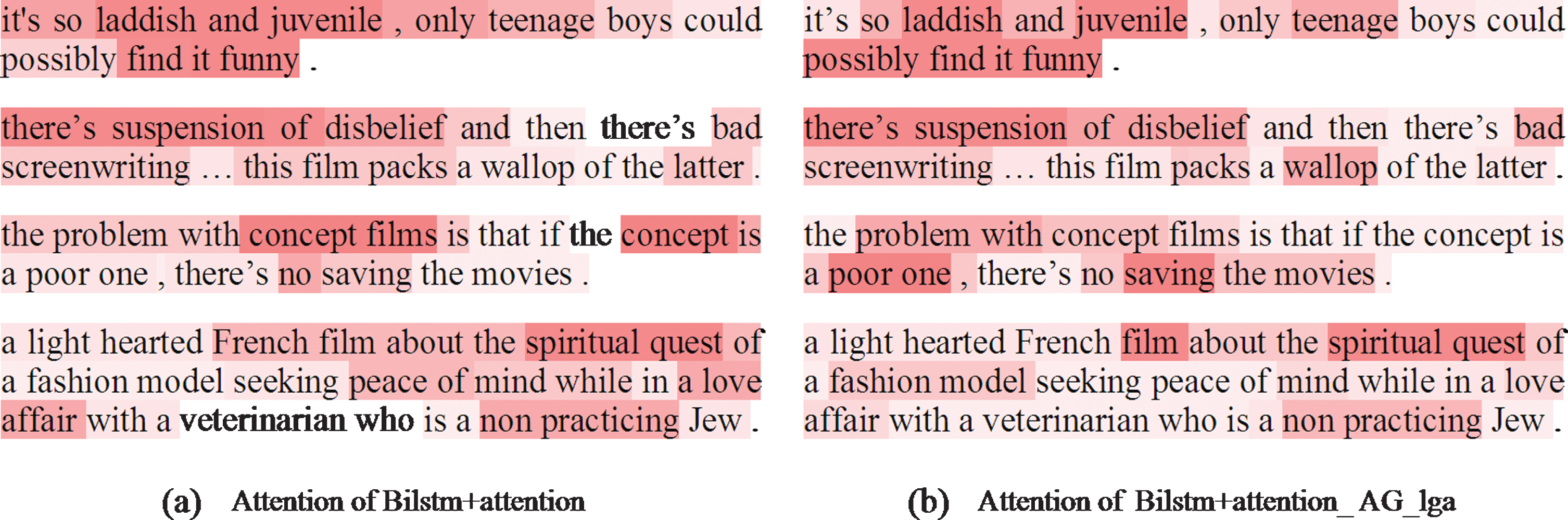
Visual representation of the attention values.
Table 2 lists the training time for the ten experimental networks to achieve accuracy. It indicates that, in most cases, the training time of the improved network is shorter than that of the original network. According to statistical data, the introduction of GAM has shortened the training time of 5.87% and 8.75% on the Bilstm+attention and the Transformer on average. Since the forward propagation process of Transformer requires more attention values than the Bilstm+attention, the use of GAM has a greater impact on it, and the training time is reduced more. The results also demonstrate that the degree of GAM optimization is strange on different datasets.
To understand the role of GAM in the training process, this paper presents the curves of the accuracy of the models on MR and TREC datasets varying with time as shown in Fig. 9.
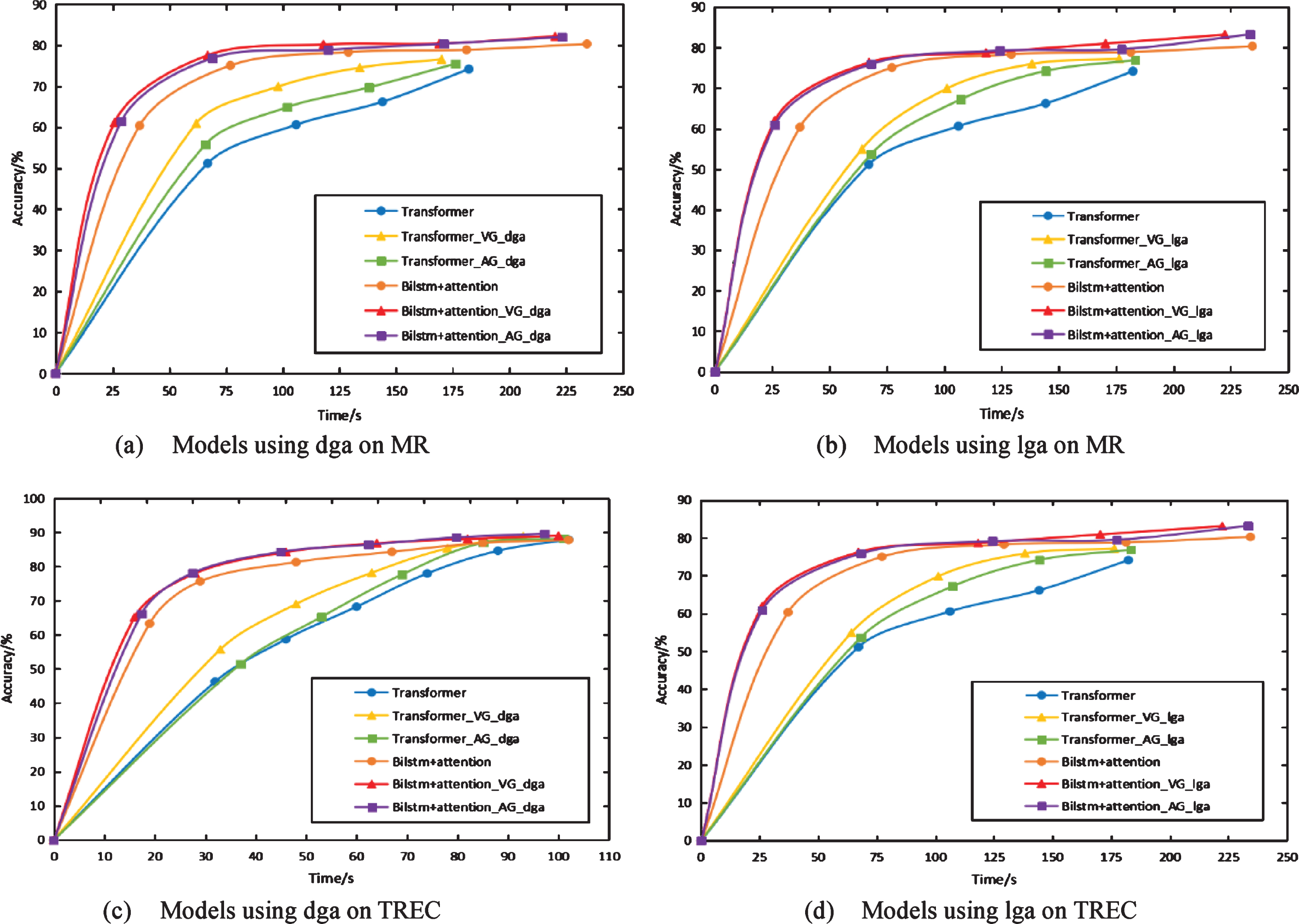
Accuracy curve over time.
In Fig. 9, the GVs generated in different ways are used to distinguish the figures on the same dataset. There (a) and (b) show the performance of each network on the MR dataset, and (c) and (d) show the performance of each network on the TREC dataset. By comparing the figures, it is worthwhile mentioning that: GAM can make the network approach the optimal accuracy faster and help the network achieve high performance in a shorter time; VG directly operates on values, which can make the effect of GVs more obvious in the early stage of network training. However, AG consumes a little time to get close to GVs in terms of angle, so it will take longer; The use of lga has a greater impact on the performance of Transformer, while the difference between lga and dga on Bilstm+attention network is not obvious.
In this work, two sets of processes for generating guiding values (GVs) are designed based on the emotional dictionary and the deep learning network. At the same time, we raise two methods combining GVs to guide the network’s attention values in terms of values and angles. The results of experiments show that Guided Attention Mechanism (GAM) can improve the performance of the attention networks. On the one hand, compared with the original network, the improved network can converge to a higher accuracy and the GVs generated by the two methods can put a good impact on the networks. On the other hand, the method of guiding angle can improve the accuracy of classification better than the method of guiding numerical value, while the latter is more advantageous in shortening the training time of network. Moreover, it is also shown in the result that the more times the attention values are generated during the forward propagation of taught network, the more significant the effect of GAM is.
Benefit by the simple and efficient operation. GAM, which has a strong generalization, enables networks to form attention values quickly and accurately during training. However, the effect of this mechanism is susceptible to GVs. When the input text is more complicated, a larger emotional dictionary and more training corpora will be needed to generate GVs.
Future research will focus on using GAM in more tasks and exploring more ways to generate GVs for different needs.
Footnotes
Acknowledgments
This work was supported by the National Natural Science Foundation of China under Grants: Methodologies for Understanding Big Data and Knowledge Discovery (61836016).