Robust sparse principal component analysis by DC programming algorithm

Abstract

The classical principal component analysis (PCA) is not sparse enough since it is based on the L₂-norm that is also prone to be adversely affected by the presence of outliers and noises. In order to address the problem, a sparse robust PCA framework is proposed based on the min of zero-norm regularization and the max of L_p-norm (0 < p ≤ 2) PCA. Furthermore, we developed a continuous optimization method, DC (difference of convex functions) programming algorithm (DCA), to solve the proposed problem. The resulting algorithm (called DC-LpZSPCA) is convergent linearly. In addition, when choosing different p values, the model can keep robust and is applicable to different data types. Numerical simulations are simulated in artificial data sets and Yale face data sets. Experiment results show that the proposed method can maintain good sparsity and anti-outlier ability.

Keywords

Principal component analysis sparseness robustness zero-norm DC programming face reconstruction

1 Introduction

Principal Component Analysis (PCA) [1] has a wide range of applications in pattern recognition, multivariate statistical analysis and machine learning [2, 3]. Classical PCA attempts to search for a set of principal components (PCs) which is obtained by maximizing variance after data projection [4]. In addition, PCs are irrelevant, which is conducive to the statistical analysis of the data after dimension reduction. However, the classical PCA is a linear combination based on the L₂-norm, which expands easily the effect of outliers and noises on the data [5, 6]. To overcome these shortcomings, improvements of methods are constantly explored.

Based on the consideration of robustness, the L₁-norm is usually used in sparse learning and robust learning [7 –9]. Kwak [10] proposed a PCA learning framework by the L₁-norm maximization, called as PCA-L₁, where the greedy algorithm was used to transform the problem into a single PC problem. The algorithm proposed by Kwak is straightforward, easy to calculate and implement. Then Kawk [11] developed a PCA by extending L₁-norm to L_p-norm (called PCA-L_p),where p is any non-negative number.In addition, PCs tend to have non-zero weight coefficients [12], which makes classical PCA not sparse enough, and interpretability worse in some applications. A variety of methods for sparsity have been developed [13 –15]. For example, Jolliffe [13] directly introduced Lasso penalty into principal component analysis, which enables automatically selection of original variables of PCA. Zou et al. [14] introduced a PCA learning framework based on elastic net. To further achieve both robustness and sparsity, Meng et al. [16] maximized the variance of the data by the L₁-norm, called RSPCA. This algorithm is easy to implement and the computational speed greatly exceeds the existing sparse PCA method. And the RSPCA has robust performance for data with inherent outliers and noises. Shao et al. [17] proposed a robust and sparse PCA-L_p (called LpSPCA) by replacing the L₁-norm with the L_p-norm, which guarantees the sparsity of PCs and verifies the robustness of the algorithm in numerical experiments, where the model can be implemented using a simple iterative algorithm.

In this paper, we propose a new sparse PCA based on zero-norm (called L_p-ZSPCA), where intends to maximize the variance of the data under L_p-norm (p ≥ 0). Unlike using the L₁-norm to approximate the L₀-norm, we apply a Gaussion function η (·) function to approximate the L₀-norm with good approximation. However, nonconvexity of the η (·) makes the problem difficult to optimize. A continuous optimization method is developed to solve the proposed framework. The problems are reformulated as DC (difference of convex functions) programming. The corresponding DC algorithms (called DC-LpZSPCA) converge linearly. Experiments on the artificial data and Yale face with outliers and noises show that the proposed LpZSPCA (0 < p ≤ 2) has a good advantage in sparsity and robustness compared to traditional PCA and other methods. Choosing different p values, DC-LpZSPCA can achieve different results.

The structure of this paper is as follows: The second section introduces the related work; in the third section we propose two new sparse PCA models and algorithms; Numerical experimentations on different datasets are shown in Section 4. The conclusions summarize the main contributions and future directions.

2 Related researches

Let X = [x₁, x₂, . . . , x_N] ∈ R^d×N be the input data matrix, where d denotes the dimension and N is the number of the given data. Transforming a location, we can assume that every ${x_{i}}_{i = 1}^{N}$ has zero mean.

The conventional PCA seeks a m (< d) dimensional linear subspace to maximize the variance of the input data. Such a subspace can be obtained by solving the following optimization

$\begin{matrix} max_{W} \sum_{i = 1}^{N} | | W^{T} x_{i} | |_{2}^{2} \\ s . t . W^{T} W = I \end{matrix}$ (1) Where || · ||₂ denotes the L₂-norm of a vector or matrix, and I ∈ R^m×m is the m × m identity matrix. W = [w₁, w₂, . . . , w_m] ∈ R^d×m, where the each column w_j of W is the j-th principal component (PC) of the original data, j = 1, 2, . . . , m. Under the constraint W^TW = I, the ${w_{j}}_{j = 1}^{m}$ is m orthonormal projection vectors. The global optimal solution of Equation (1) can be found by singular value decomposition (SVD).

From statistical perspectives, the L₁-norm is more robust to outliers than the L₂-norm. So, substituting the L₂-norm in Equation (1), the L₁-norm was put to use in the variance function [10], where a greedy algorithm is used to attain a local optimal solution. This approach reduces the influence of the outliers and it is invariant to rotations [10]. With an arbitrary non-integer value, the L_p-norm (p > 0) is applied in PCA study [11], which leads to following optimization.

$\begin{matrix} max_{W} \frac{1}{p} \sum_{i = 1}^{N} | | W^{T} x_{i} | |_{p}^{p} = \frac{1}{p} \sum_{i = 1}^{N} \sum_{j = 1}^{m} {| w_{j}^{T} x_{i} |}^{p} \\ s . t . W^{T} W = I \end{matrix}$ (2) It is easy to see that Equation (2) lacks interpretation and yields PCA to be not sparse enough. Then Shao et al proposed a sparse PCA model [17]:

$\begin{matrix} max_{W} \frac{1}{p} \sum_{i = 1}^{N} | | W^{T} x_{i} | |_{p}^{p} = \frac{1}{p} \sum_{i = 1}^{N} \sum_{j = 1}^{m} {| w_{j}^{T} x_{i} |}^{p} \\ s . t . W^{T} W = I, | | W | |_{1} \leq k, p > 0 \end{matrix}$ (3) Here || · ||₁ denotes L₁-norm and k is defined by user that controls the sparsity. However, the solution for the problem Equation (2)3 is not sparse enough.

3 Mainly contributions

3.1 A Robust sparse principal component analysis

In order to enforce sparsity and robustness, we propose a new PCA learning framework, called L_p-ZSPCA,(p > 0):

$\begin{matrix} max_{W} λ \frac{1}{p} \sum_{i = 1}^{N} | | W^{T} x_{i} | |_{p}^{p} - (1 - λ) ∥ W ∥_{0} \\ s . t . W^{T} W = I \end{matrix}$ (4) where λ ∈ (0, 1) is a parameter and || · ||₀ denotes L₀-norm. In objective function, the first term is to maximize the sample variance in a projection subspace by L_p-norm (p > 0); the second term is to minimize ∥W ∥ ₀ whose goal is to control the sparsity of the projection subspace. Equation (4) aims at receiving sparse PCs based on maximizing the variance of the input data X. Different values of p fit various data types.

To find m principal components, Equation (4) is reformulated as

$\begin{matrix} max_{W} λ \frac{1}{p} \sum_{i = 1}^{N} \sum_{j = 1}^{m} {| w_{j}^{T} x_{i} |}^{p} - (1 - λ) ∥ W ∥_{0} \\ s . t . W^{T} W = I \end{matrix}$ (5) Note that the objective function in Equation (5) is non-convex and thus it is difficult to optimize since the zero-norm is nonconvex. The L₁-norm is only a convex proximation for zero-norm, but minimizing the L₁-norm generates many components that are close to zero, but not exactly equal to zero.

In this work, we apply a generalized the zero-norm that is a Laplace kernel-based function η (·) to approximate the zero-norm ∥ · ∥ ₀ [18]. With different parameters, the Gaussion function η (·) is illustrated in Fig. 1. The closer the parameter is to positive infinity, the more approximate the Gaussion function is to the zero-norm.

Fig. 1

Approximations to L₀-norm for the Gaussion function η (x) and L₁-norm.

3.2 DC-LpZSPCA algorithm for one sparse PC

We first consider L_p-ZSPCA with one principal component. With m = 1, we obtain L_p-ZSPCA with one PC

$\begin{matrix} max_{w} λ \frac{1}{p} \sum_{i = 1}^{N} {| w^{T} x_{i} |}^{p} - (1 - λ) ∥ w ∥_{0} \\ s . t . w^{T} w = 1 \end{matrix}$ (6) We focus on the cases in which m = 1 to obtain the PC1 first. And then, we can use a greedy algorithm to get more than one projection vectors (m > 1). However, Equation (6) is a nonconvex and discontinuous optimization. We first relax nonconvex constraint w^Tw = 1 into convex constraint w^Tw ≤ 1, and then obtain discontinuous optimization $\begin{matrix} min_{w} (1 - λ) | | w | |_{0} - λ \frac{1}{p} \sum_{i = 1}^{N} | w^{T} x_{i} |^{p} \\ s . t . | | w | |_{2} \leq 1 \end{matrix}$ (7) which is equivalent to the following problem:

$\begin{matrix} max_{W} F_{p} (w) = \frac{1}{p} \sum_{i = 1}^{N} | w^{T} x_{i} |^{p} \\ s . t . w^{T} w \leq 1, | | w | |_{0} ⩽ k \end{matrix}$ (8) Here, k represents sparse degree defined by user. The gradient of F_p (w) denotes ▽_w (F)

$▽_{w} (F) = \sum_{i = 1}^{N} sgn (w^{T} x_{i}) | w^{T} x_{i} |^{p - 1} x_{i}$ (9)

For minimizing ||w||₀, Equation (8) can be reformulated as the following optimization.

$\begin{matrix} min_{w} (1 - λ) | | w | |_{0} - λ \frac{1}{p} \sum_{i = 1}^{N} | w^{T} x_{i} |^{p} \\ s . t . | | w | |_{2} \leq 1 \end{matrix}$ (10)

A good approximation [20] of the ||w||₀ would be

$| | w | |_{0} \approx \sum_{i = 1}^{d} η (w_{i}, α);$ (11) Here, for $x \in R$ , η (x) function is defined by

$η (u) = 1 - ɛ^{- α | u |}, α > 0, u \in R$ (12) Note that η (u) can be remained as a DC function [19, 20] η (u) = g (u) - h (u)

with

$g (u) = α | u |, h (u) = α | u | - 1 + ɛ^{- α | u |}$ (13) where g (u), h (u) are the DC components of η (x), and they are convex functions. ɛ is an exponential constant. The zero-norm of vector $w \in R^{d}$ can be approximated by

$| | w | |_{0} ≃ \sum_{i = 1}^{N} η (w_{i}, α) = \sum_{i = 1}^{d} (1 - ɛ^{- α | w_{i} |})$ (14) Here, α ∈ R, α > 0.

Compared with other approximation of the zero-norm such as

$C_{α} (z) = 1 - e^{- α z^{2}}, (α > 0)$ (15) the approximation accuracy of the η (·) function is higher than that of the C_α (·) function, and the details refer to the literature [21].

The objective function of Equation (10) can be reformulated as

$N_{p} (w) = G (w) - H (w)$ (16)G (w) and H (w) are both convex functions, and

$\begin{matrix} G (w) = (1 - λ) \sum_{j = 1}^{N} g (w_{j}) \\ H (w) = (1 - λ) \sum_{j = 1}^{N} h (w_{j}) + λ \frac{1}{p} \sum_{i = 1}^{N} | w^{T} x_{i} |^{p} . \end{matrix}$ (17)

Assuming that Ω is the feasible set of Equation (10) and χ_Ω (x) is the indicator function for the convex set Ω: $χ_{Ω} (x) = {\begin{matrix} 0 & x \in Ω \\ + \infty & x \notin Ω \end{matrix}$ Therefore, the Equation (10) can be reformulated as the following DC programming:

$min {G (w) + χ_{Ω (w)} - H (w)}$ (18) The gradient of H (w) is as following.

$\begin{matrix} \nabla H (w_{j}) = & α (1 - λ) sgn (w_{j}) (1 - ɛ^{- α | w_{j} |}) \\ + λ \nabla_{w_{j}} (F) \end{matrix}$ (19) Here, sgn (·) denotes the sign function, ∇_{w
_j} (F) denotes the j-th element of ∇_w (F).

According to the generic DCA scheme, at each iteration l, we need to compute ▿H (w^l) and deal with the following convex programming to obtain the solution w^l+1

$min_{w} {G (w) + χ_{Ω (w)} - ▿ H (w^{l})^{T} w}$ (20) Then by introducing variable t satisfying |w| ≤ t, Equation (20) equals to dealing with the following SOCP for α > 0.

$\begin{matrix} min_{w, t} α (1 - λ) e^{T} t - ▿ H (w^{l})^{T} (w - w^{l}) \\ s . t . | | w | |_{2} \leq 1, - t \leq w \leq t \end{matrix}$ (21) Here α > 0, w ∈ R^d. This is a second order cone programming (SOCP) and using the interior algorithm, this optimization can be solve in polynomial time.

Although the approximation of Equation (14) is closer to the L₀-norm than the L₁-norm, the Equation (14) also generates many components that are close to zero but not exactly equal to zero because of the limitations of approximation. So we sort w by the absolute value of the value and get w₁, w₂, . . . , w_n. Let γ > 0 and γ = w_k+1. In other words, γ is the (k + 1)-th largest number of |w|, where k represents data sparsity. Based on Equation (21), the solution w need to be changed by the following state.

$w = {\begin{matrix} w_{j} & | w_{j} | \geq γ \\ 0 & | w_{j} | < γ \end{matrix}$ (22)

In what follows, we describe the DC algorithm of LpZSPCA when m = 1.

Theorem

Algorithm 1 generates a sequence ${{\hat{w}}^{(l)}}$ such that $G ({\hat{w}}^{(l)}) - H ({\hat{w}}^{(l)})$ decreases monotonously.

The sequence ${{\hat{w}}^{(l)}}$ converges linearly.

Proof. These conclusion can be directly proved by the convergence properties of general DC program. The proof is then completed.□

3.3 DC algorithm of LpZSPCA for m principal components

The greedy algorithm is used in this section. The basic idea is to obtain the first PC1 (w₁) by applying the algorithm 1 to original data, and then project the data into the space that is orthogonal to vector w₁ to get the new data set. After that, based on the projection data, we continue to apply algorithm 1 to obtain PC2 and then get the m-th principal component.

Algorithm 1 DC-LpZSPCA(m =1) (Input: X, p, k, Output: w^*)

1: α > 0 and λ ∈ (0, 1) is fixed.

2: δ > 0 is sufficiently small and set l = 0. Choose an initial point w⁰ ∈ Ω;

3: Singularity check:

if p<0 and ∃ i: w^T^(l)x_i = 0, then w^(l) ← (w^(l) + ρ)/||w^(l) + ρ||₂, where ρ is a small random vector;

4: Compute ▿H (w^(l)) via (19);

5: Solve the SOCP (21) to obtain w^(l+1);

6: Let γ be the (k+1)-th largest element of |w|. According to the (21), get the $\hat{w}$ .

7: Convergence check:

a) If $| | {\hat{w}}^{(l + 1)} - {\hat{w}}^{(l)} | | > δ$ or $G ({\hat{w}}^{(l + 1)}) - H ({\hat{w}}^{(l + 1)}) \leq G ({\hat{w}}^{(l)}) - H ({\hat{w}}^{(l)}) - δ$ , return to Step 2.

b) Else, $w^{*} \leftarrow {\hat{w}}^{(l)}$ . Stop iteration.

The PCs do not vary if the value of m changes. PC1 is local optimal solution of Equation (5) by Algorithm 1 and PCs (m > 1) are local suboptimal solution of Equation (5) by Algorithm 2. What’s more, the orthogonality of ${w_{i}}_{i = 1}^{m}$ cannot be ensured in theory. Algorithm 2 is a heuristic algorithm and we just can obtain the approximate solution of Equation (5).

Algorithm 2 DC-LpZSPCA algorithm(m >1) (Input: X, m and k. Output: ${w_{j}}_{i = 1}^{m}$ )

1: δ > 0 is sufficiently small and set k = 0.

Choose an initial point w⁰ ∈ Ω and $X^{0} = {x_{i}^{0} = x_{i}}_{i = 1}^{n}$ ;

2: For j-th principal component, j = 1, 2, . . . , m

a), let data point $X^{j} = {x_{i}^{j}}_{i = 1}^{N} = {x_{i}^{j - 1} - \frac{{w^{*}}_{j - 1} {w^{*}}_{j - 1}^{T} x_{i}^{j - 1}}{| | w_{j - 1}^{*} | |_{2}}}_{i = 1}^{N}$ ;

b) Apply Algorithm 1 on X_j

3: Apply algorithm 1 in dataset X to obtain the j-th principal component w_j, (j = 2, ⋯ , m).

4 Experiment results

In order to verify the proposed LpZSPCA and its DC algorithm, especially the robustness in noises setting, the traditional PCA [1], RSPCA [16], PCA-L_p [11] with p = 0.5, 1, 1.5, 2 and LpSPCA [17] with p = 0.5, 1, 1.5, 2 methods have been used as the benchmark methods. For the sake of convenience, we use the name of LpPCA instead of PCA-L_p. All programs were completed in Matlab 2018, and the experiments used the popular package SeDuMi as a solver. The implementation environment was the personal computer with 2.3 GHz Intel Core i5.

4.1 Parameter selection

The choice of parameters will affect the final result. There are three parameters, k, α, λ in the proposed DC-LpZSPCA method. The sparsity k can be well selected according to the characteristics of data set. Later, the grid search method is adopted to determine parameters, α and λ. It is proved in the literature [19] that a good value of λ in Equation (21) using the zero-norm is better to be larger than 0.5. But it also depends on the dataset type, so we consider the values λ < 0.5 as well. In this work, we suggest using the following set of candidate values in our experiments: $\begin{matrix} α \in {50, 10, 5, 1, 0.5, 0.1} \\ λ \in {0.9, 0.8, 0.7, 0.6, 0.5, 0.3, 0.1, 0.05, 0.0001} \end{matrix}$

In order to observe intuitively the sensitivity on different parameters λ and α, for yale face dataset with occluded noise and p = 0.5, we draw a graph (see Fig.2) that shows the reconstruction error (ARCE) varies with the parameters λ and α. According to the Fig.2, we find the ARCE increases when λ ranges from 0.0001 to 0.9, and that the ARCE produces greater values when α is set to a large value.

Fig. 2

The sensitive analysis on parameters λ and α.

4.2 A toy problem with four outliers

We design a three-dimensional toy dataset $(x_{i}, y_{i}, z_{i})_{i = 1}^{31}$ with four outliers to verify the robust performance of the DC-LpZSPCA when p has different values. In this section, dataset is constructed using the literature [17].

The data is generated by picking x_i ∈ [-3, 3], and yielding y_i and z_i from the uniform distribution on [0,0.1] and [-1,-0.9] respectively, which is approximately parallel to the x-axis. In order to further verify the robustness of the algorithm, two sets with outliers will be introduced, whose coordinates are expressed as (4 + α_i, 2 + β_i, 4 + γ_i) and (α_i, - 3 + β_i, 4 + γ_i) respectively,here, α_i, β_i, γ_i are randomly taken from the uniform distribution on interval [0,0.1], i = 1, 2.

The artificial data set is composed of a main direction parallel to the x axis and four outliers deviating from the main direction. The essence of the data set is a one-dimension vector in three-dimension space. Therefore, this set will test the robust effect of above methods. The selection of parameters is as follows. The sparsity k of RSPCA and DC-LpZSPCA is set to 2. When p takes from the set {0.5, 1, 1.5, 2}, λ takes from the set {0.05, 0.002, 0.001, 0.004} respectively and α takes from the set {0.1, 5, 5, 0.5} respectively.

To further explore the robustness of the algorithm, we introduce the concept of the average residual error, called ARSE.

$\bar{e} = \frac{1}{N} | | ζ_{i} - {ww}^{T} ζ_{i} | |_{2}$ (23)

Here, ζ_i = {(x_i, y_i, z_i)} is the i-th data point; w is the first PC vector and N is the number of the data set.

Projection direction of the first PCs of the proposed LpZSPCA (p = 0.5, 1, 1.5, 2) and traditional PCA is shown in Fig. 3. The ARSEs conducted by PCA, RSPCA, LpPCA, LpSPCA and LpZSPCA methods are presented in Table 1. The results from Fig. 3 present that the PC1 direction obtained by DC-LpZSPCA (p = 1.5) is closest to the true direction of the data; when p = 1 or 2, the influence of the outliers increases. Compared with the traditional PCA, the DC-LpZSPCA (p = 1, 1.5, 2) methods are closer to the real direction. When p = 0.5, it is the closest to the projection direction of the traditional PCA.

Fig. 3

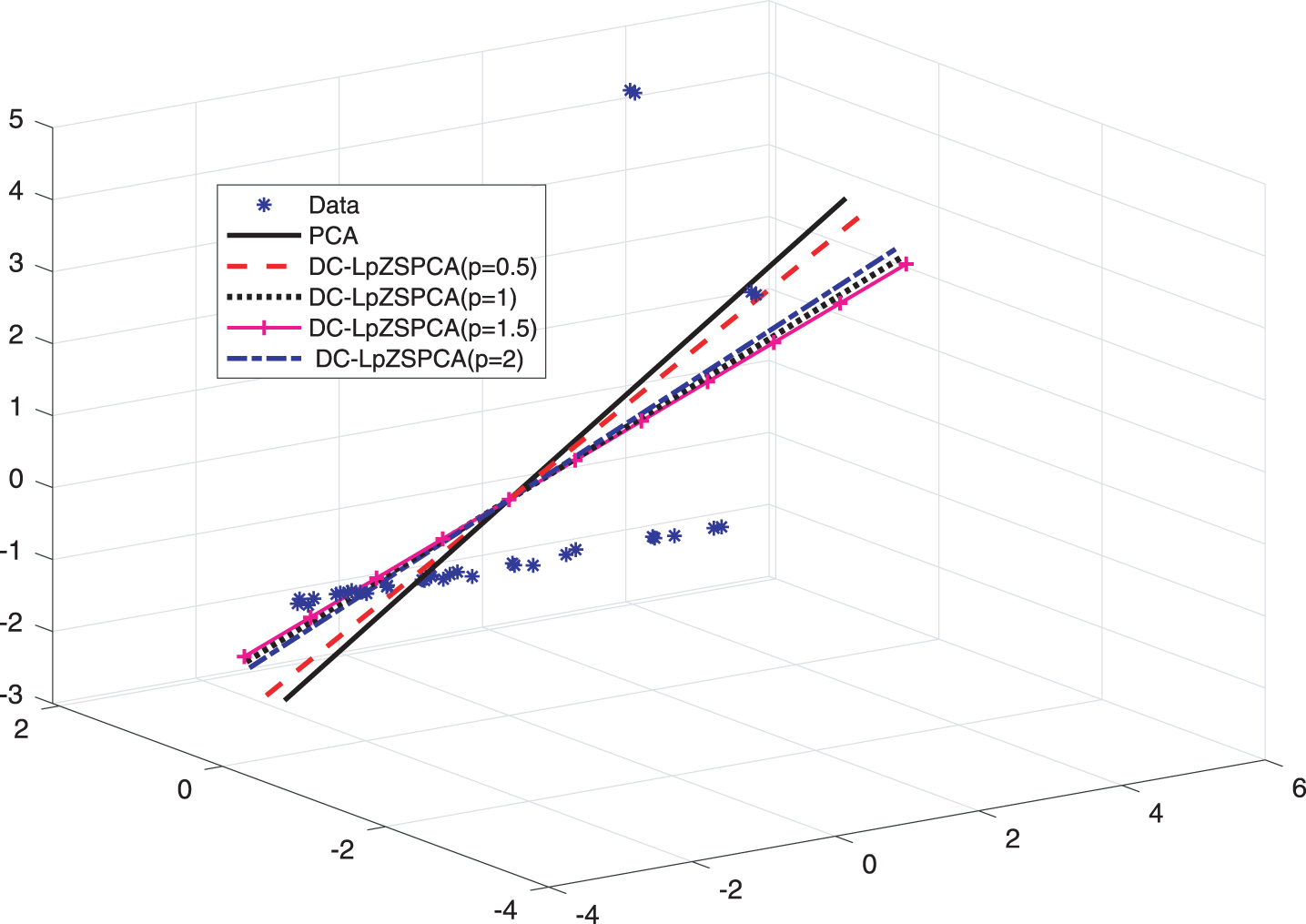
The first PCs obtained by the PCA and DC-LpZSPCA respectively in toy data.

Table 1

PC1s and the ARSE of 5 methods

Methods	PC1	ARSE
PCA	(0.8506,0.0593,0.5225)	1.0882
RSPCA	(0.8820,0,0.4712)	1.0459
LpPCA (p = 0.5)	(0.7267,-0.0634,0.6840)	1.2185
LpPCA (p = 1)	(0.874,-0.0370,0.4845)	1.0600
LpPCA (p = 1.5)	(0.8645,0.0017,0.5027)	1.0636
LpPCA (p = 2)	(0.8417,0.0552,0.5371)	1.0947
LpSPCA (p = 0.5)	(0.8772,0,0.4801)	1.0503
LpSPCA (p = 1)	(0.8820,0,0.4712)	1.0459
LpSPCA (p = 1.5)	(0.8647,0,0.5023)	1.0633
LpSPCA (p = 2)	(0.8520,0,0.5236)	1.0771
DC-LpZSPCA (p = 0.5)	(0.8467,0,0.5311)	1.0822
DC-LpZSPCA (p = 1)	(0.916,0,0.4011)	1.0306
DC-LpZSPCA (p = 1.5)	(0.9240,0,0.3824)	1.0322
DC-LpZSPCA (p = 2)	(0.9054,0,0.4245)	1.0318

According to Table 1, it is found that ARSE of DC-LpZSPCA (p = 0.5, 1, 1.5, 2) is smaller than PCA. When p = 1, the ARSE of DC-LpZSPCA is the smallest among all methods. When p value is fixed, the average residual error of DC-LpZSPCA is smaller than that of LpPCA and LpSPCA except for p = 0.5. These results show that DC-LpZSPCA has good robustness with different values of p (p ≤ 2).

4.3 Synthetic data

In this section we produce the artificial dataset similar to literature [14]. This is a set of ten-dimensional datasets generated by the following steps:

First define three potential factors:

V₁∼N (0, 160)

V₂∼N (0, 200)

V₃ = -0.1V₁ + 0.88V₂ + ε

where ε∼N (0, 1), and V₁, V₂ and ε are independent of each other. x_i is denoted the i-th feature of the data points, (i = 1, 2, . . . , 10). The x_i (i = 1, 2, 3, 4) take from V₁; x_i (i = 5, 6, 7, 8) take from V₂; x₉ and x₁₀ take from V₃.

The variance of the three underlying factors is 160, 200, 156.48, respectively. The numbers of the data variables related to the three factors are 4, 4, 2. Hence V₁ and V₂ are almost equally significantly, and they are much more important than V₃. The article data itself has a certain degree of sparsity.

The algorithms (PCA, RPCA, LpPCA, LpSPCA, DC-LpZSPCA) are applied to the data, and the results are shown in Tables 2 and 3. It can be seen intuitively that the standard PCA and LpPCA (p = 0.5, 1, 1.5, 2) are not sparse, and RSPCA, LpSPCA and DC-LpZSPCA (p = 0.5, 1, 1.5, 2) is sparse. At the same time, when p = 0.5, DC-LpZSPCA is closed to the true value. Because it can be calculated that the ARSE of the different methods. The ARSE value of DC-LpZSPCA(p = 0.5) is 91.13 but the ARSE values of other methods are not above 80.

Table 2
Loadings of the first two PCs by PCA and RSPCA

PCA RSPCA

PC1 PC2 PC1 PC2

-0.4808 0.0943 0.5490 0

-0.4598 0.1100 0.4835 0

-0.4701 0.0995 0.4497 0

-0.4763 0.1002 0.5124 0

-0.0841 -0.5076 0 0.5311

-0.0886 -0.4842 0 0.5286

-0.0765 -0.4787 0 0.4709

-0.0720 -0.4732 0 0.4656

0.2040 0.0839 0 0

0.2049 0.0830 0 0

PCA	RSPCA
-0.4808	0.0943	0.5490	0
-0.4598	0.1100	0.4835	0
-0.4701	0.0995	0.4497	0
-0.4763	0.1002	0.5124	0
-0.0841	-0.5076	0	0.5311
-0.0886	-0.4842	0	0.5286
-0.0765	-0.4787	0	0.4709
-0.0720	-0.4732	0	0.4656
0.2040	0.0839	0	0
0.2049	0.0830	0	0

Table 3

Loadings of the first two PCs by LpPCA, LpSPCA and DC-LpZSPCA

LpPCA(p = 0.5)		LpPCA(p = 1)		LpPCA(p = 1.5)		LpPCA(p = 2)
PC1	PC2	PC1	PC2	PC1	PC2	PC1	PC2
0.2719	0.3584	0.2923	0.3570	0.3492	-0.2726	0.4426	0.1627
0.2479	0.3424	0.2666	0.3430	0.2983	-0.2852	0.4238	0.1332
0.2498	0.3766	0.2720	0.3631	0.2956	-0.3024	0.4307	0.1374
0.2482	0.3695	0.2700	0.3644	0.3157	-0.2954	0.4394	0.1383
0.3940	-0.0517	0.3892	-0.0873	0.4108	0.2832	-0.0066	0.4407
0.3502	-0.0158	0.3500	-0.0561	0.3930	0.2506	0.0060	0.4038
0.3379	-0.0288	0.3391	-0.0667	0.3723	0.2503	-0.0034	0.39340
0.3649	-0.0385	0.3618	-0.0801	0.3684	0.2590	-0.0133	0.4107
0.3240	-0.4894	0.2937	-0.4853	-0.0366	0.4501	-0.3499	0.3448
0.3323	-0.4808	0.3007	-0.4827	-0.0550	0.4362	-0.3511	0.3430
LpSPCA(p = 0.5)		LpSPCA(p = 1)		LpSPCA(p = 1.5)		LpSPCA(p = 2)
PC1	PC2	PC1	PC2	PC1	PC2	PC1	PC2
0.5454	0.0443	0.7542	-0.0019	0	0.5858	0.5490	0
0	0.6383	0.4218	0	0	0.4825	0.4835	0
0	0.4873	0.0056	0.6537	0	0.3942	0.4497	0
0.0131	0.5942	0.5031	0	0	0.5183	0.5124	0
0	0	0	0	0.5025	0	0	0.5311
0	0	0	0	0.6112	0	0	0.5286
0	0	0	0	0.4440	0	0	0.4709
0	0	0	0	0.4204	0	0	0.4656
-0.2448	0	0	-0.5370	0	0	0	0
-0.8015	0	0	-0.5332	0	0	0	0
DC-LpZSPCA(p = 0.5)		DC-LpZSPCA(p = 1)		DC-LpZSPCA(p = 1.5)		DC-LpZSPCA(p = 2)
PC1	PC2	PC1	PC2	PC1	PC2	PC1	PC2
0	0.4432	0	0.5287	0	0.5172	0.5444	0
0	0.4776	0	0.5049	0	0.5020	0.4015	0
0	0.3907	0	0.4408	0	0.4666	0.4329	0
0	0.4012	0	0.4888	0	0.4949	0.4582	0
0.5226	0	0.5612	0	0.4201	0	0	0.7022
0.3830	0	0.4667	0	0.3811	0	0	0.4427
0.3698	0	0.4427	0	0.3639	0	0	0.3392
0.4478	0	0.4897	0	0.3804	0	0	0.4426
0	0	0	0	0	0	0	0
0	0	0	0	0	0	0	0

4.4 Face reconstruction problems

The dataset used in this paper is the famous Yale face dataset which includes 165 gray faces, containing 11 different expressions of 15 volunteers. The dataset is available from the official website http://cvc.yale.edu/projects/yalefaces/yale-faces.html. The size of the original image is 320 pixels × 243 pixels. In this experiment, the original image is normalized as the image of 100 pixels ×100 pixels.

In order to test the robustness of DC-LpZSPCA, we add occluded noise and dummy noise to the Yale data respectively [16]. The specific processing method is as follows:

Occluded noise: Randomly select two images from each of the 15 volunteers’ face images. Then use a rectangular noise with black and white dots at random positions, whose size was 70 pixels ×30 pixels or 40 pixels ×60 pixels.

Dummy noise: Use black and white noise to create a picture of the same size as the face after cropping, and record it as a virtual picture. Then we add 30 virtual pictures to the original data set.

In this paper, the reconstructed feature face and the average reconstruction error are used as test indicators to detect the robustness of the DC-LpZSPCA algorithm. In this paper, the first m principal components (PCs) are selected to reconstruct the image, and the average reconstruction error (ARCE) is expressed as:

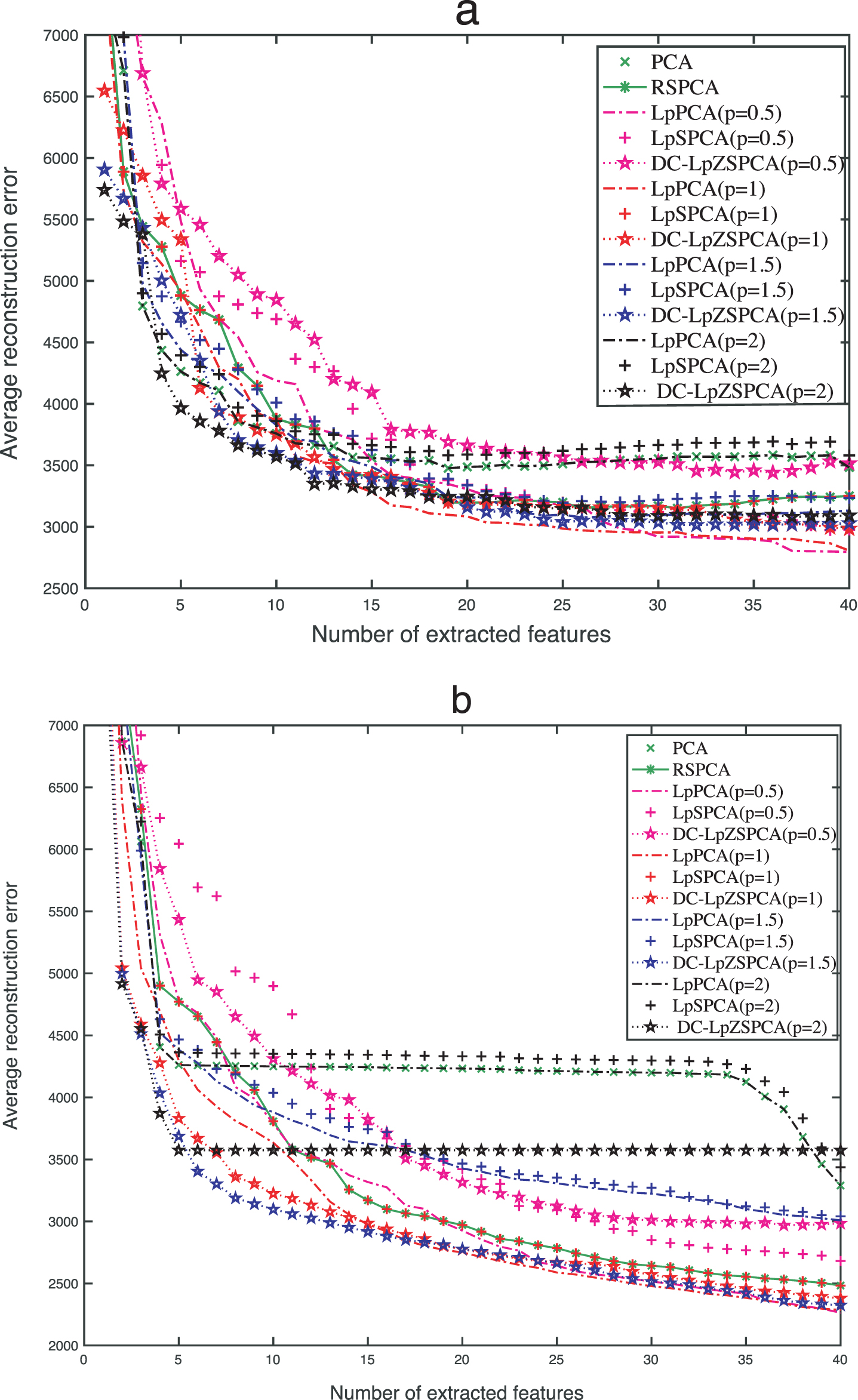
$e (m) = \frac{1}{n} \sum_{i = 1}^{n} | | ξ_{i}^{0} - \sum_{j = 1}^{m} w_{j} w_{j}^{T} ξ_{i} | |_{2}$ (24) Here, n is the number of image samples, $ξ_{i}^{0}$ means the i-th original face, and ξ_i means the face data after the noise reduction.

For yale face datasets with two kinds of noises, we extracted 20 PCs to create the reconstructed images by PCA, RSPCA, LpPCA, LpSPCA, and DC-LpZSPCA, and the results are shown in the Figs. 5 and 6 respectively. At the same time, the ARCE tendency curves are shown in Fig. 4, which illustrates the above 5 methods with various numbers of extracted PCs in occluded and dummy cases, respectively. Here, the optimal parameters of DC-LpZSPCA are obtained under different noises with different p values. Under occluded noise with k = 9500, p takes from {0.5, 1, 1.5, 2}; λ takes from {0.9, 0.7, 0.5, 0.001}; α takes from {1, 0.5, 0.5, 0.1} respectively. Under dummy noise with k = 9500, p takes from {0.5, 1, 1.5, 2}, λ takes from {0.7, 0.3, 0.3, 0.7}, and α takes from {0.5, 0.1, 0.5, 1} respectively.

Fig. 4

The ARCE Tendency curves for occluded (a) and dummy (b) Yale images respectively.

Fig. 5

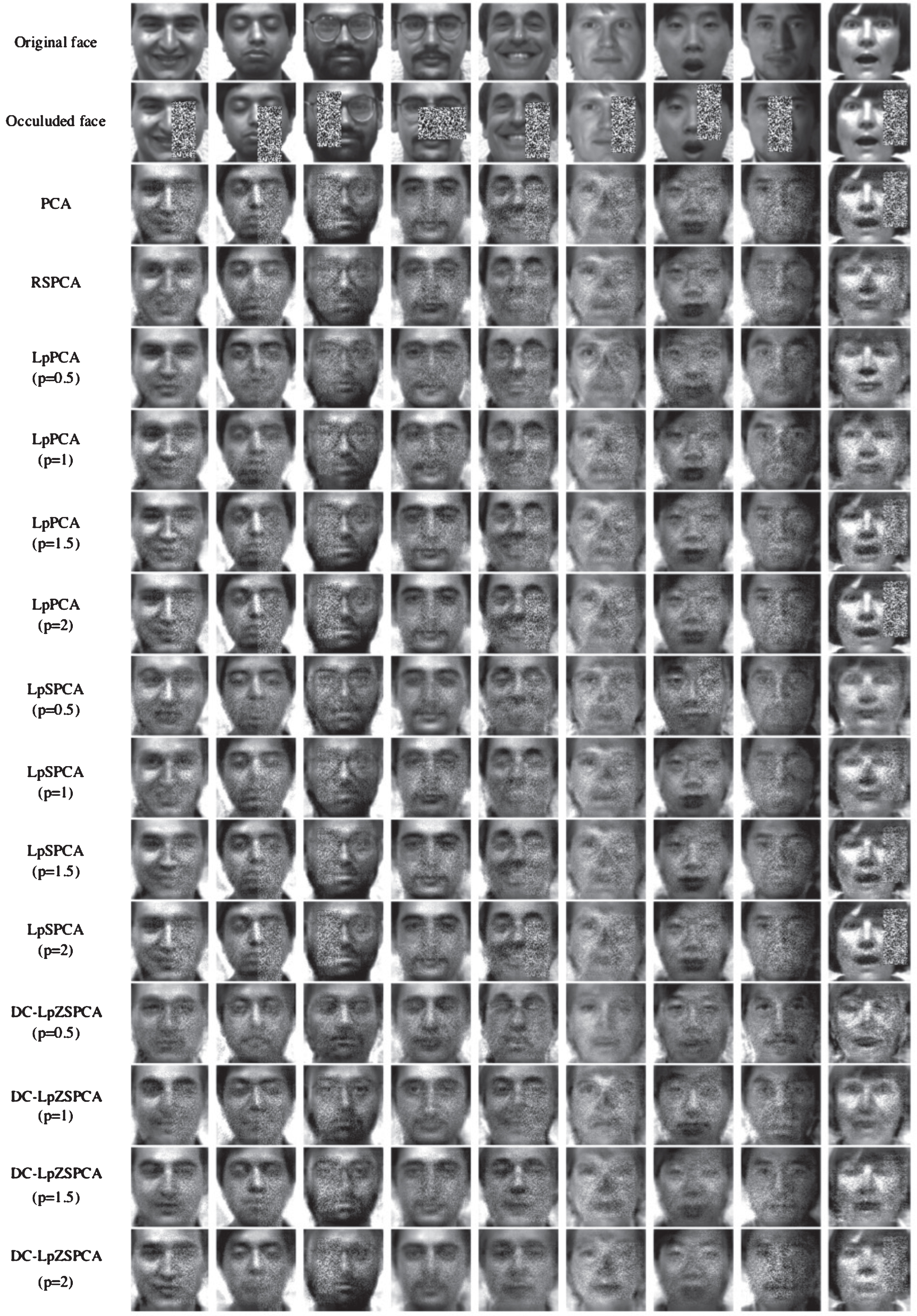
The original face images, the corresponding images with occluded noise, and the faces reconstructed by the classic PCA, RSPCA, LpPCA, LpSPCA and DC-LpZSPCA methods with 20 corresponding projection PCs, respectively.

Fig. 6

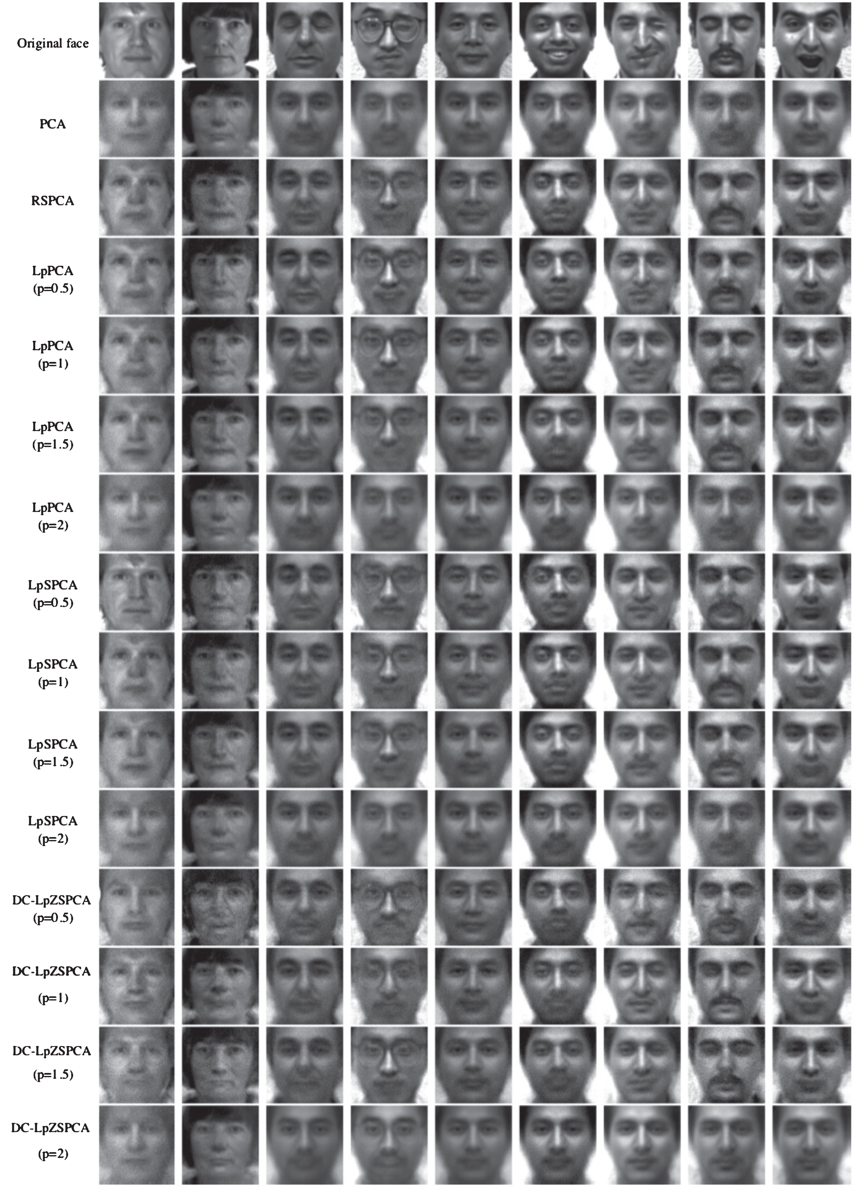
The original face images, the corresponding images with dummy noise, and the faces reconstructed by the classic PCA, PSPCA, LpPCA, LpSPCA and DC-LpZSPCA methods with 20 corresponding projection PCs, respectively.

For occluded case, Fig. 5 illustrates the face reconstruction images in occluded case, where it is seen that the faces reconstructed by the DC-LpZSPCA algorithm is closest to the original face. Although the RSPCA method has fewer noise points, the detailed shape and expression are quite different from the original face images. Comparing to the LpPCA method, for a fixed p, the reconstructed images by DC-LpSPCA are with higher resolution than that by other methods (PCA, RSPCA, LpPCA and LpSPCA).

In Fig. 4 (a), when the number of extracted features m is less than 15, the average reconstruction error computed by DC-LpSPCA with p = 2 is significantly smallest among all algorithms. As the number of principal components increases, the values of ARCE for DC-LpZSPCA with p = 1, 1.5, 2 are very close to the minimum value. And the DC-LpZSPCA achieves better sparsity without loss of ARCE. At the same time, we know that DC-LpZSPCA with p = 0.5 has unsatisfactory ARCE values.

In Fig. 4 (b), the value of ARCE of DC-LpZSPCA with p = 1.5 is the smallest in all methods when m < 5. When 5 ≤ m < 15, the ARCE value of DC-LpZSPCA with p = 1.5 is very close to the minimum. As m increases, the values of ARCE of DC-LpZSPCA are only slightly higher than the minimum and tends to be stable.

For dummy case, it is found in Fig. 6 that the reconstructed faces of PCA, LpPCA (p = 2) and DC-LpZSPCA (p = 2) are the most blurred and do not show the characteristics of each face. Relatively speaking, RSPCA, LpPCA (p = 1) and DC-LpZSPCA (p = 1.5, p = 1) are more successful in reproducing the original face image, and the details of eyes, glasses, beard and so on are well presented.

5 Conclusion

In this work, a sparse robust PCA is proposed based on the zero-norm regularization and the p-norm (0 < p ≤ 2) PCA. Following that, a continuous optimization method, DC programming algorithm (called DC-LpZSPCA), is developed to solve the proposed sparse L_p-ZSPCA. The resulting DC optimization algorithm converges linearly. Numerical experimentations are carried out on an artificial data sets and Yale face data sets, and the results show that the proposed DC-LpZSPCA can maintain good sparsity and anti-outlier effect, compared with the traditional PCA methods in most cases.

Footnotes

Acknowledgments

This work is supported by National Nature Science Foundation of China (No.11471010 and No.11271367).

References

Jolliffe

I.T.

, Principal Component Analysis, Springer-Verlag, New York, NY, 1986.

Jolliffe

I.T.

and Cadima

, Principal component analysis: A review and recent developments, Philos Trans Roy Soc A, Math, Phys Eng Sci 374(2065) (2016), 20150202.

Seghouane

A.K.

, Shokouhi

and Koch

, Sparse Principal Component Analysis with Preserved Sparsity Pattern, IEEE Transactions on Image Processing 28(7) (2019), 3274–3285.

and Chen

S.B.

, compressive principal component analysis, Front Comput Sci 14(4) (2020), 144303.

, Zhu

and Lu

, Principal component analysis based on block-norm minimization, Appl Intell 49(6) (2019), 2169–2177.

Menon

T.V.

and Kalyani

, Structured and Unstructured Outlier Identification for Robust PCA: A Fast Parameter Free Algorithm, IEEE Transactions on Signal Processing 67(9) (2019), 2439–2452.

and Kanade

, Robust L1-norm factorization in the presence of outliers and missing data by alternative convex programming, IEEE Computer Society Conference on Computer Vision and Pattern Recognition (2005), 739–746.

Brooks

J.P.

, Dul

J.H.

and Boone

E.L.

, A pure L1-norm principal component analysis, Computational Statistics and Data Analysis (2013), 83–98.

Ding

, Zhou

, He

X.F.

and Zha

H.Y.

, R1-PCA: rotational invariant L1-norm principal component analysis for robust subspace factorization, Proc 23rd Int Conf Machine Learning (2006), 281–288.

10.

Kwak

, Principal component analysis based on L1-norm maximization, IEEE Transactions on Pattern Analysis and Machine Intelligence (2008), 1672–1680.

11.

Kwak

, Principal component analysis by Lp-norm maximization, IEEE Transactions on Cybernetics (2014), 594–609.

12.

, Jiusun

and Lei

, Structured Joint Sparse Principal Component Analysis for Fault Detection and Isolation, IEEE Transactions on Industrial Informatics 15(5) (2019), 2721–2731.

13.

Journee

, Nesterov

, Richtarik

and Sepulchre

, Generalized power method for sparse principal component analysis, Journal of Machine Learning Research 11(2008070) (2010), 517–553.

14.

Zou

, Hastie

and Tibshirani

, Sparse principal component analysis, Journal of Computational and Graphical Statistics (2006), 265–286.

15.

Sigg

C.D.

and Buhmann

J.M.

, Expectation maximization for sparse and non-negative PCA, ACM, Helsinki, Finland, (2008), 960–967.

16.

Meng

D.Y.

, Zhao

and Xu

Z.B.

, Improve robustness of sparse PCA by L1-norm maximization, Pattern Recognition 45(1) (2012), 487–497.

17.

C.H.

, Chen

and Shao

, Robust sparse Lp-norm Principal Component Analysis, Acta Automatica Sinica 43(1) (2017), 142–151.

18.

Yang

and Qian

, A sparse logistic regression framework by difference of convex functions programming, Applied Intelligence 45 (2016), 241–254.

19.

Nguyen

and Baets

, An approach to supervised distance metric learning based on difference of convex functions programming, Pattern Recognition 81 (2018), 562–574.

20.

Yang

and Siyun

, A sparse extreme learning machine framework by continuous optimization algorithms and its application in pattern recognition, Engineering Applications of Artificial Intelligence 53 (2016), 176–189.

21.

Yang

, Ren

, Wang

, et al., A Robust Regression Framework with Laplace Kernel-Induced Loss, Neural Computation 29(11) (2017), 3014–3039.