Parameter estimation in uncertain differential equations with exponential solutions

Abstract

This paper proposes three methods to estimate the parameters in uncertain differential equations (UDEs) based on discrete observation data. The first method is designed for a class of UDEs in which their solutions have the explicit expressions of uncertainty distribution. The second method is given to solve the estimation problem through the inverse uncertainty distribution. In the third method, the unknown parameters of UDEs are estimated by the solution of the corresponding α-path. These methods are interpreted to be efficient and practical by using a popular UDE with exponential solutions and obtaining the detailed estimators of the parameters.

Keywords

Uncertain differential equation uncertainty distribution inverse uncertainty distribution

1 Introduction

The concept of uncertain differential equation (UDE) was first proposed by Liu [1]. Chen and Liu [2] obtained the analytic solution of a linear UDE. The solution problem of UDEs was also studied by Liu [3], Yao [4], Liu [5], Wang [6], Yao and Chen [7], and Zhou and Li [8]. More details of UDEs refer to Gao [9], Liu [10], and Yao et al. [11].

In the past few years, uncertain differential equations were widely used to model dynamic uncertain systems that are subject to uncertain fluctuations, such as finance. For example, Liu [10] proposed an uncertain stock model by uncertain differential equation and derived its European option price formulas. Chen and Gao [12] introduced an uncertain interest rate model. Chen [13] obtained the American option pricing formula for uncertain financial market. Yao [14] discussed an application in stock model with floating interest rate, and Liu [15] studied uncertain currency model. Moreover, uncertain differential equation has also been introduced to study optimal control, see Zhu ([16], [17]). Recently, Li et al. [18] firstly applied uncertain differential equation to the domain of infectious diseases, and established an uncertain SIS epidemic model. Fang et al. [19] obtained the solution and α-path of uncertain SIS model with standard incidence and demography. Li et al. [20] compared with deterministic, stochastic and uncertain SIS epidemic models, and revealed the relationship among them. Up to now, uncertain differential equations are becoming increasingly important due to the application for modelling uncertain phenomena in different fields.

Since there always exist some unknown parameters in UDEs, it is key to obtain the estimated values of unknown parameters in order to investigate the properties of UDEs. Li [21] used the least-square method to estimate unknown parameters of a class of simple UDEs as follows $\begin{matrix} {dX}_{t} = (α_{0} + \sum_{l = 1}^{p} α_{l} F_{l} (t)) dt + β {dC}_{t}, X_{0} = x_{0}, \end{matrix}$ where α_l (l = 0, 1, …, p), β (≠0) are unknown parameters, and C_t is an uncertain process. However, the estimation problem of unknown parameters for other uncertain differential equations is seldom studied. In this paper, we propose three approaches to estimate the unknown parameters in general UDEs.

The rest is arranged as follows. In Sect. 2, we review some basic definitions of uncertain differential equation. Three methods are proposed to estimate unknown parameters of UDEs under different conditions in Sect. 3. Based on the proposed methods, we obtain the formulas of the estimated parameters for UDEs with exponential solutions in Sect. 4, and conclusions are given in Sect. 5.

2 Definitions

Let $L$ be a σ-algebra on a non-empty set Γ. Every element $Λ \in L$ is called an event.

Definition 1. [22] A set function $M$ : $L \to [0, 1]$ is called an uncertain measure if it is supposed to satisfy four axioms:

Axiom 1 (Normality Axiom) $M {Γ} = 1$ for the universal set Γ.

Axiom 2 (Duality Axiom) $M {Λ} + M {Λ^{c}} = 1$ for any event Λ.

Axiom 3 (Subadditivity Axiom) For every countable sequence of events Λ₁, Λ₂, . . . , $M {⋃_{i = 1}^{+ \infty} Λ_{i}} \leq \sum_{i = 1}^{+ \infty} M {Λ_{i}} .$ The triplet $(Γ, L, M)$ is called an uncertainty space.

Axiom 4 (Product Axiom) Let $(Γ_{i}, L_{i}, M_{i})$ be uncertainty spaces and Λ_i be arbitrarily chosen events from $L_{i}$ for i = 1, 2, . . . , then the product uncertain measure $M$ is an uncertain measure satisfying $M {\prod_{i = 1}^{+ \infty} Λ_{i}} = ⋀_{i = 1}^{+ \infty} M_{i} {Λ_{i}} .$

Definition 2. [22] An uncertain variable ξ is a measurable function from uncertainty space $(Γ, L, M)$ to the set of real numbers $ℝ$ ; that is, for any Borel set B of $ℝ$ , the set {ξ ∈ B} = {γ ∈ Γ|ξ (γ) ∈ B} is an event.

Definition 3. [22] For any real number $x \in ℝ$ , uncertainty distribution Φ of uncertain variable ξ is defined by $Φ (x) = M {ξ \leq x}$ .

Definition 4. [23] An uncertainty distribution Φ (x) is said to be regular if it is a continuous and strictly increasing function with respect to x at which 0 < Φ (x) <1, and $lim_{x \to - \infty} Φ (x) = 0, lim_{x \to + \infty} Φ (x) = 1 .$

Definition 5. [23] Let ξ be an uncertain variable with regular uncertainty distribution Φ (x). Then, the inverse function Φ^-1 (α) is called inverse uncertainty distribution of ξ.

An uncertain variable ξ is said to be normal if it has uncertainty distribution $\begin{matrix} Φ (x) = (1 + exp (\frac{π (e - x)}{\sqrt{3} σ}))^{- 1}, x \in ℝ, \end{matrix}$ denoted by $ξ \sim N (e, σ)$ , where e and σ are real numbers with σ > 0. Especially, if e = 0 and σ = 1, ξ is called standard normal, denoted by $ξ \sim N (0, 1)$ .

Definition 6. [1] Let T be an index set, and $(Γ, L, M)$ be an uncertainty space. An uncertain process X_t is a measurable function from $T \times (Γ, L, M)$ to the set of real numbers, i.e., for each t ∈ T and any Borel set B of real numbers, the set {X_t ∈ B} = {γ|X_t (γ) ∈ B} is an event.

Definition 7. [24] An uncertain process X_t is said to have an uncertainty distribution Φ_t (x), if the uncertain variable X_t has the uncertainty distribution _t (x) at any time t.

Definition 8. [10] An uncertain process C_t is said to be Liu process, if

(i) C₀ = 0 and almost all sample paths are Lipschitz continuous.

(ii) C_t has stationary and independent increments.

(iii) Every increment C_t+s - C_s is a normal uncertain variable with an uncertainty distribution $Φ_{t} (x) = (1 + exp (- \frac{π x}{\sqrt{3} t}))^{- 1}, x \in ℝ .$

Definition 9. [10] Let X_t be an uncertain process and C_t be Liu process. For any partition of closed interval [a, b] with a = t₁ < t₂ < ⋯ < t_k+1 = b, the mesh is written as $△ = max_{1 \leq i \leq k} | t_{i + 1} - t_{i} |$ . Then, Liu integral of X_t is defined by $\int_{a}^{b} X_{t} {dC}_{t} = lim_{△ \to 0} \sum_{i = 1}^{k} X_{t_{i}} \cdot (C_{t_{i + 1}} - C_{t_{i}})$ provided that the limit exists almost surely and is finite.

Definition 10. [1] Let f and g be two given functions. Then ${dX}_{t} = f (t, X_{t}) dt + g (t, X_{t}) {dC}_{t}$ (1) is called an uncertain differential equation (UDE). An uncertain process X_t is called a solution of UDE (1), if X_t satisfies the UDE (1) for any time t.

The uncertain differential equation (1) is equivalent to the uncertain integral equation $X_{t} = X_{0} + \int_{0}^{t} f (s, X_{s}) ds + \int_{0}^{t} g (s, X_{s}) {dC}_{s} .$

Definition 11. [7] Let α be a number with 0 < α < 1. An uncertain differential equation (1) is said to have an α-path $X_{t}^{α}$ if it solves the corresponding ordinary differential equation ${dX}_{t}^{α} = f (t, X_{t}^{α}) dt + | g (t, X_{t}^{α}) | Φ^{- 1} (α) dt,$ where Φ^-1 (α) is the inverse standard normal uncertainty distribution, that is $Φ^{- 1} (α) = \frac{\sqrt{3}}{π} ln \frac{α}{1 - α} .$ (2)

3 Estimation methods

3.1 Estimation based on uncertainty distribution

Consider an uncertain differential equation as follows

$\begin{matrix} {dX}_{t} = f (t, X_{t}; a) dt + g (t, X_{t}; b) {dC}_{t}, X_{0} = x_{0}, \end{matrix}$ (3) where a and b are two unknown parameters. For the equation (3), we introduce a method based on uncertainty distribution to estimate the unknown parameters, denoted by Method I. The process of this method is formed by the following steps.

Step 1. Calculate the analytic solution X_t of UDE (3), denoted by X_t = S₁ (t, C_t).

Step 2. Let Ψ_{X
_t} (x, t ; a, b) be uncertainty distribution of the solution X_t at any time t. By Definitions 3 and 7, we have $Ψ_{X_{t}} (x, t; a, b) = M {X_{t} \leq x} = M {S_{1} (t, C_{t}) \leq x}$ for $x \in ℝ$ and t > 0. By Definition 8, $C_{t} \sim N (0, t)$ . If the expression of Ψ_{X
_t} (x, t ; a, b) can be obtained, we denote it as F (x, t ; a, b), that is, Ψ_{X
_t} (x, t ; a, b) = F (x, t ; a, b) .

Step 3. Let Ψ_{X
_t} (x_i, t_j) be the observations of Ψ_{X
_t} (x, t ; a, b) for i = 1, 2, …, n and j = 1, 2, …, m. Define the error $e_{ij} = Ψ_{X_{t}} (x_{i}, t_{j}) - F (x_{i}, t_{j}; a, b),$ which is the deviation of the observed value from the true value of Ψ_{X
_t} (x, t ; a, b).

Step 4. By the least-square method, the values $\hat{a}$ and $\hat{b}$ of a and b need to satisfy

$min_{a, b} \sum_{i = 1}^{n} \sum_{j = 1}^{m} e_{ij}^{2} = min_{a, b} \sum_{i = 1}^{n} \sum_{j = 1}^{m} (Ψ_{X_{t}} (x_{i}, t_{j}) - F (x_{i}, t_{j}; a, b))^{2} .$

The solutions $\hat{a}$ and $\hat{b}$ are called the least-square estimators based on uncertainty distribution Ψ_{X
_t} (x, t ; a, b), denoted by UD-LS estimators $\hat{a}$ and $\hat{b}$ for short.

3.2 Estimation based on inverse uncertainty distribution

Suppose that the solution X_t of UDE (3) has uncertainty distribution Ψ_{X
_t} (x, t ; a, b) at any time t. If Ψ_{X
_t} (x, t ; a, b) is regular, by Definition 5, then its inverse function $Ψ_{X_{t}}^{- 1} (α, t; a, b) (α \in (0, 1))$ is the inverse uncertainty distribution of X_t. Based on the expression of $Ψ_{X_{t}}^{- 1} (α, t; a, b)$ , we introduce a method to estimate two unknown parameters a and b, called Method II. The method includes the processes below.

Step 1. The first step is similar to that of Method I. The analytic solution X_t of UDE (3) is denoted by X_t = S₁ (t, C_t).

Step 2. From Definitions 3 and 7, we have $Ψ_{X_{t}} (x, t; a, b) = M {S_{1} (t, C_{t}) \leq x}$ for $x \in ℝ$ and t > 0. Suppose the uncertainty distribution Ψ_{X
_t} (x, t ; a, b) is regular. If the inverse uncertainty distribution $Ψ_{X_{t}}^{- 1} (α, t; a, b)$ can be obtained, we denote it as G (α, t ; a, b).

Step 3. Let $Ψ_{X_{t}}^{- 1} (α_{i}, t_{j})$ be the observations of $Ψ_{X_{t}}^{- 1} (α, t;$ a, b) for i = 1, 2, …, n and j = 1, 2, …, n. Define the error $γ_{ij} = Ψ_{X_{t}}^{- 1} (α_{i}, t_{j}) - G (α_{i}, t_{j}; a, b),$ which is the deviation of the observed value from the true value of $Ψ_{X_{t}}^{- 1} (α, t; a, b)$ .

Step 4. By the least-square method, the solutions of $\begin{matrix} min_{a, b} \sum_{i = 1}^{n} \sum_{j = 1}^{m} γ_{ij}^{2} \\ = min_{a, b} \sum_{i = 1}^{n} \sum_{j = 1}^{m} (Ψ_{X_{t}}^{- 1} (α_{i}, t_{j}) - G (α_{i}, t_{j}; a, b))^{2} \end{matrix}$ are called the least-square estimators based on inverse uncertainty distribution, denoted as IUD-LS estimators a′ and b′.

3.3 Estimation based on α-path

Next, we introduce the third method based on α-path to estimate unknown parameters of a type of UDEs when their uncertainty distributions, or inverse uncertainty distributions are too difficult to solve. The method based on α-path of UDE is called Method III. The process is divided into four steps.

Step 1. By Definition 11 of α-path, an α-path $X_{t}^{α}$ of UDE (3) is given by an ordinary differential equation

$\frac{{dX}_{t}^{α}}{dt} = f (t, X_{t}^{α}; a) + | g (t, X_{t}^{α}; b) | Φ^{- 1} (α),$ (4) where Φ^-1 (α) is defined in (2) for α ∈ (0, 1).

Step 2. Calculate the solution $X_{t}^{α}$ of (3), denoted by $X_{t}^{α} = S_{2} (t, α; a, b)$ for 0 < α < 1.

Step 3. Let $X_{t_{j}}^{α_{i}}$ be observations from S₂ (t, α ; a, b) for i = 1, 2, …, n, j = 1, 2, …, m and α_i ∈ (0, 1). In order to approximately solve $X_{t}^{α} = S_{2} (t, α; a, b)$ , define the error $ε_{ij} = X_{t_{j}}^{α_{i}} - S_{2} (t_{j}, α_{i}; a, b),$ which is the deviation of the observed value from the true value of S₂ (t, α ; a, b).

Step 4. By the least-square method, the estimated values satisfy

$min_{a, b} \sum_{i = 1}^{n} \sum_{j = 1}^{m} ε_{ij}^{2} = min_{a, b} \sum_{i = 1}^{n} \sum_{j = 1}^{m} (X_{t_{j}}^{α_{i}} - S_{2} (t_{j}, α_{i}; a, b))^{2},$

which are called the least-square estimators based on α-path $X_{t}^{α}$ , denoted as α-path LS estimators $\tilde{a}$ and $\tilde{b}$ .

4 Parameter estimation of UDEs with exponential solutions

In order to illustrate our proposed estimation methods, we consider a UDE with exponential solutions

${dX}_{t} = a X_{t} dt + b X_{t} {dC}_{t}$ (5) with X₀ = x₀ (>0), where a and b are unknown non-zero parameters. From Definition 10, the solution of the UDE is an uncertain process

$X_{t} = x_{0} exp (at + b C_{t}) .$ (6) It can be seen that X_t > 0 for any t > 0.

Theorem 1. Let Ψ_{X
_t} (x, t ; a, b) be the uncertainty distribution of the uncertain process (6). For any x > 0 and t > 0, we have $Ψ_{X_{t}} (x, t; a, b) = {[1 + exp (- \frac{π (ln x - ln x_{0} - at)}{\sqrt{3} | b | t})]}^{- 1} .$ (7)

Proof. By Definitions 3 and 7 of uncertainty distribution, for any x > 0, we have $\begin{matrix} Ψ_{X_{t}} (x, t; a, b) \\ = M {X_{t} \leq x} = M {x_{0} exp (at + b C_{t}) \leq x} \\ = M {b C_{t} \leq ln x - ln x_{0} - at} . \end{matrix}$

(i) If b > 0, by Definition 8, then $\begin{matrix} Ψ_{X_{t}} (x, t; a, b) \\ = M {C_{t} \leq \frac{1}{b} (ln x - ln x_{0} - at)} \\ = {[1 + exp (- \frac{π (ln x - ln x_{0} - at)}{\sqrt{3} bt})]}^{- 1} . \end{matrix}$

(ii) If b < 0, then $\begin{matrix} Ψ_{X_{t}} (x, t; a, b) \\ = M {C_{t} \geq \frac{1}{b} (ln x - ln x_{0} - at)} \\ = 1 - M {C_{t} < \frac{1}{b} (ln x - ln x_{0} - at)} \\ = 1 - {[1 + exp (- \frac{π (ln x - ln x_{0} - at)}{\sqrt{3} bt})]}^{- 1} \\ = {[1 + exp (\frac{π (ln x - ln x_{0} - at)}{\sqrt{3} bt})]}^{- 1} . □ \end{matrix}$

Corollary 1. The uncertainty distribution Ψ_{X
_t} (x, t ; a, b) of the uncertain process X_t is regular at each time t.

Proof. For each time t, we have $lim_{x \to - \infty} Ψ_{X_{t}} (x, t; a, b) = M {X_{t} \leq x} = 0$ because of X_t > 0 for any time t. From Theorem 1,

$\begin{matrix} lim_{x \to + \infty} Ψ_{X_{t}} (x, t; a, b) \\ = & lim_{x \to + \infty} {[1 + exp (- \frac{π (ln x - ln x_{0} - at)}{\sqrt{3} | b | t})]}^{- 1} = 1 . \end{matrix}$

Thus, by Definition 4, the uncertainty distribution Ψ_{X
_t} (x, t) is regular. □

Corollary 2. Both uncertain processes X_t = x₀ exp(at + bC_t) and Y_t = x₀ exp(at - bC_t) have the same uncertainty distribution.

Let y_i = (y_i1, y_i2, …, y_im), t_i = (t_i1, t_i2, …, t_im), u_i = (u_i1, u_i2, …, u_im) and ɛ_i = (ɛ_i1, ɛ_i2, …, ɛ_im) for i = 1, 2, …, n. Denote $\begin{matrix} Y & = & (y_{1}, y_{2}, \dots, y_{n})^{T}, \\ U & = & {(\begin{matrix} t_{1} & t_{2} & \dots & t_{n} \\ u_{1} & u_{2} & \dots & u_{n} \end{matrix})}^{T}, \end{matrix}$ (8) $ɛ = (ɛ_{1}, ɛ_{2}, \dots, ɛ_{n})^{T} .$ and θ = (θ₁, θ₂) ^T, where the superscript T represents transpose of a vector or matrix. Based on the expressions of Y, U, ɛ and θ, we establish a model $y_{ij} = θ_{1} t_{ij} + θ_{2} u_{ij} + ɛ_{ij}$ for i = 1, 2, …, n and j = 1, 2, …, m, where θ_i (i = 1, 2) are unknown parameters, and ɛ_ij are mutually independent residual terms. In matrix form,

$Y = U θ + ɛ .$ (9) Suppose the inverse matrix (U^TU) ^-1 exists. The least-squares method is used to estimate the unknown parameters of the model (9).

Lemma 1. Let $\hat{θ} = ({\hat{θ}}_{1}, {\hat{θ}}_{2})^{T}$ be the least-square estimator of θ in the model (9). Then, $\begin{matrix} {\begin{matrix} {\hat{θ}}_{1} = & \frac{\sum_{i = 1}^{n} \sum_{j = 1}^{m} y_{ij} u_{ij} \sum_{i = 1}^{n} \sum_{j = 1}^{m} u_{ij} t_{ij} - \sum_{i = 1}^{n} \sum_{j = 1}^{m} y_{ij} t_{ij} \sum_{i = 1}^{n} \sum_{j = 1}^{m} u_{ij}^{2}}{(\sum_{i = 1}^{n} \sum_{j = 1}^{m} u_{ij} t_{ij})^{2} - \sum_{i = 1}^{n} \sum_{j = 1}^{m} t_{ij}^{2} \sum_{i = 1}^{n} \sum_{j = 1}^{m} u_{ij}^{2}}, \\ \hat{θ_{2}} = & \frac{\sum_{i = 1}^{n} \sum_{j = 1}^{m} y_{ij} t_{ij} \sum_{i = 1}^{n} \sum_{j = 1}^{m} u_{ij} t_{ij} - \sum_{i = 1}^{n} \sum_{j = 1}^{m} t_{ij} \sum_{i = 1}^{n} \sum_{j = 1}^{m} y_{ij} u_{ij}}{(\sum_{i = 1}^{n} \sum_{j = 1}^{m} u_{ij} t_{ij})^{2} - \sum_{i = 1}^{n} \sum_{j = 1}^{m} t_{ij}^{2} \sum_{i = 1}^{n} \sum_{j = 1}^{m} u_{ij}^{2}} . \end{matrix} \end{matrix}$

Proof. For the model (9), the least-square function is $\begin{matrix} Q (θ) & = & \sum_{i = 1}^{n} \sum_{j = 1}^{m} ɛ_{ij}^{2} = ɛ^{T} ɛ = (Y - U θ)^{T} (Y - U θ) \\ = & Y^{T} Y - 2 Y^{T} U θ + θ^{T} U^{T} U θ . \end{matrix}$ In order to minimize Q, we have $\begin{matrix} \frac{\partial Q}{\partial θ} = - 2 Y^{T} U + 2 U^{T} U θ = 0 . \end{matrix}$ Let $c = \sum_{i = 1}^{n} \sum_{j = 1}^{m} t_{ij}^{2} \sum_{i = 1}^{n} \sum_{j = 1}^{m} u_{ij}^{2} - (\sum_{i = 1}^{n} \sum_{j = 1}^{m} u_{ij} t_{ij})^{2}$ . The least-square estimator $\hat{θ}$ is

$\begin{matrix} \hat{θ} & = & (\begin{matrix} {\hat{θ}}_{1} \\ {\hat{θ}}_{2} \end{matrix}) = (U^{T} U)^{- 1} U^{T} Y \\ = & \frac{1}{c} (\begin{matrix} \sum_{i = 1}^{n} \sum_{j = 1}^{m} u_{ij}^{2} & - \sum_{i = 1}^{n} \sum_{j = 1}^{m} u_{ij} t_{ij} \\ - \sum_{i = 1}^{n} \sum_{j = 1}^{m} u_{ij} t_{ij} & \sum_{i = 1}^{n} \sum_{j = 1}^{m} t_{ij}^{2} \end{matrix}) U^{T} Y \\ = & \frac{1}{c} (\begin{matrix} \sum_{i = 1}^{n} \sum_{j = 1}^{m} y_{ij} t_{ij} \sum_{i = 1}^{n} \sum_{j = 1}^{m} u_{ij}^{2} - \sum_{i = 1}^{n} \sum_{j = 1}^{m} y_{ij} u_{ij} \sum_{i = 1}^{n} \sum_{j = 1}^{m} u_{ij} t_{ij} \\ \sum_{i = 1}^{n} \sum_{j = 1}^{m} t_{ij}^{2} \sum_{i = 1}^{n} \sum_{j = 1}^{m} y_{ij} u_{ij} - \sum_{i = 1}^{n} \sum_{j = 1}^{m} y_{ij} t_{ij} \sum_{i = 1}^{n} \sum_{j = 1}^{m} u_{ij} t_{ij} \end{matrix}) . □ \end{matrix}$

4.1 Method I

Without loss of generality, suppose b > 0 in (6) based on Corollary 2. Thus, by Theorem 1, we have $\begin{matrix} \frac{\sqrt{3}}{π} ln \frac{Ψ_{X_{t}} (x, t; a, b)}{1 - Ψ_{X_{t}} (x, t; a, b)} = - \frac{a}{b} + \frac{ln x - ln x_{0}}{bt} . \end{matrix}$

Let Ψ_{X
_t} (x_i, t_j) be observations of uncertainty distribution Ψ_{X
_t} (x, t ; a, b) for i = 1, 2, …, n and j = 1, 2, …, m. Define the error $e_{ij} = \frac{\sqrt{3}}{π} ln \frac{Ψ_{X_{t}} (x_{i}, t_{j})}{1 - Ψ_{X_{t}} (x_{i}, t_{j})} + \frac{a}{b} - \frac{ln x_{i} - ln x_{0}}{{bt}_{j}} .$ It follows that the optimization problem is

$min_{a, b} \sum_{i = 1}^{n} \sum_{j = 1}^{m} e_{ij}^{2}$ (10) $= min_{a, b} \sum_{i = 1}^{n} \sum_{j = 1}^{m} (\frac{\sqrt{3}}{π} ln \frac{Ψ_{X_{t}} (x_{i}, t_{j})}{1 - Ψ_{X_{t}} (x_{i}, t_{j})} + \frac{a}{b} - \frac{ln x_{i} - ln x_{0}}{{bt}_{j}})^{2},$

where the unknown parameters a and b are the solution of the minimization of problem. By solving the optimization problem (10), it is to obtain the following result.

Theorem 2. For UDE (5), the UD-LS estimators of parameters a and b are $\begin{matrix} \begin{matrix} \hat{a} & = \frac{\sum_{i = 1}^{n} \sum_{j = 1}^{m} v_{ij} \sum_{i = 1}^{n} \sum_{j = 1}^{m} (\frac{ln x_{i} - ln x_{0}}{t_{j}})^{2} - \sum_{i = 1}^{n} \sum_{j = 1}^{m} v_{ij} \frac{ln x_{i} - ln x_{0}}{t_{j}} \sum_{i = 1}^{n} \sum_{j = 1}^{m} \frac{ln x_{i} - ln x_{0}}{t_{j}}}{\sum_{i = 1}^{n} \sum_{j = 1}^{m} v_{ij} \sum_{i = 1}^{n} \sum_{j = 1}^{m} \frac{ln x_{i} - ln x_{0}}{t_{j}} - nm \sum_{i = 1}^{n} \sum_{j = 1}^{m} v_{ij} \frac{ln x_{i} - ln x_{0}}{t_{j}}}, \\ \hat{b} & = \frac{(\sum_{i = 1}^{n} \sum_{j = 1}^{m} \frac{ln x_{i} - ln x_{0}}{t_{j}})^{2} - nm \sum_{i = 1}^{n} \sum_{j = 1}^{m} (\frac{ln x_{i} - ln x_{0}}{t_{j}})^{2}}{\sum_{i = 1}^{n} \sum_{j = 1}^{m} v_{ij} \sum_{i = 1}^{n} \sum_{j = 1}^{m} \frac{ln x_{i} - ln x_{0}}{t_{j}} - nm \sum_{i = 1}^{n} \sum_{j = 1}^{m} v_{ij} \frac{ln x_{i} - ln x_{0}}{t_{j}}}, \end{matrix} \end{matrix}$ where $v_{ij} = \frac{\sqrt{3}}{π} ln \frac{Ψ_{X_{t}} (x_{i}, t_{j})}{1 - Ψ_{X_{t}} (x_{i}, t_{j})}$ for i = 1, 2, …, n and j = 1, 2, …, m.

Proof. For (8), let $y_{ij} = \frac{\sqrt{3}}{π} ln \frac{Ψ_{X_{t}} (x_{i}, t_{j})}{1 - Ψ_{X_{t}} (x_{i}, t_{j})}, u_{ij} = \frac{ln x_{i} - ln x_{0}}{t_{j}},$ and t_ij = 1 for i = 1, 2, …, n ; j = 1, 2, …, m, and $θ = (θ_{1}, θ_{2})^{T} = (- \frac{a}{b}, \frac{1}{b})^{T}$ . Thus, the optimization problem (10) is written by $\begin{matrix} min_{a, b} \sum_{i = 1}^{n} \sum_{j = 1}^{m} e_{ij}^{2} = min_{a, b} \sum_{i = 1}^{n} \sum_{j = 1}^{m} (y_{ij} - θ_{1} - θ_{2} u_{ij})^{2} . \end{matrix}$ By Lemma 1, we can obtain the UD-LS estimators $\hat{a}$ and $\hat{b}$ of a and b. □

Fig. 1

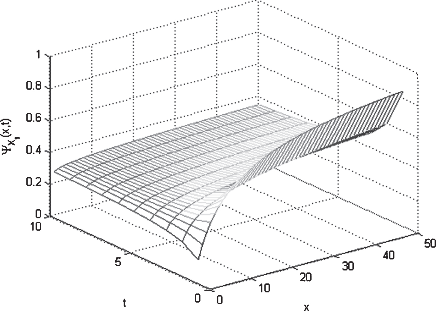
The curve of uncertainty distribution Ψ_{X
_t} (x, t) with x₀ = 3, a = 1 and b = 2.

Example 1. Take x₀ = 3, a = 1 and b = 2 in UDE (5). By Theorem 1, the uncertainty distribution Ψ_{X
_t} (x, t) of the solution X_t is $\begin{matrix} Ψ_{X_{t}} (x, t) = {[1 + exp (- \frac{π (ln x - ln 3 - t)}{2 \sqrt{3} t})]}^{- 1} \end{matrix}$

for x > 0 and t > 0 . Figure 1 provides the trajectory of Ψ_{X
_t} (x, t).

Through the grid intersections of Ψ_{X
_t} (x, t) in Figure 1, we get 500 observations Ψ_{X
_t} (x_i, t_j), where x_i = i and t_j = j for i = 1, 2, …, 50 and j = 1, 2, …, 10. Clearly, n = 50 and m = 10. Since

$\begin{matrix} \sum_{i = 1}^{n} \sum_{j = 1}^{m} \frac{\sqrt{3}}{π} ln \frac{Ψ_{X_{t}} (x_{i}, t_{j})}{1 - Ψ_{X_{t}} (x_{i}, t_{j})} = - 113.0017, \\ \sum_{i = 1}^{n} \sum_{j = 1}^{m} (\frac{ln x_{i} - ln x_{0}}{t_{j}})^{2} = 331.2799, \\ \sum_{i = 1}^{n} \sum_{j = 1}^{m} \frac{\sqrt{3}}{π} ln \frac{Ψ_{X_{t}} (x_{i}, t_{j})}{1 - Ψ_{X_{t}} (x_{i}, t_{j})} \frac{ln x_{i} - ln x_{0}}{t_{j}} = 28.6416, \end{matrix}$

$\begin{matrix} \sum_{i = 1}^{n} \sum_{j = 1}^{m} \frac{ln x_{i} - ln x_{0}}{t_{j}} = 273.9966, \end{matrix}$ by Theorem 2, we get the UD-LS estimators of a and b as follows

$\begin{matrix} \hat{a} & = & \frac{- 113.0017 \times 331.2799 - 28.6416 \times 273.9966}{- 113.0017 \times 273.9966 - 50 \times 10 \times 28.6416} = 1, \\ \hat{b} & = & \frac{(273.9966)^{2} - 50 \times 10 \times 331.2799}{- 113.0017 \times 273.9966 - 50 \times 10 \times 28.6416} = 2 . \end{matrix}$

4.2 Method II

Through Theorem 1, Corollaries 1 and 2, the inverse uncertainty distribution $Ψ_{X_{t}}^{- 1} (α, t; a, b)$ of UDE (5) is $Ψ_{X_{t}}^{- 1} (α, t; a, b) = exp (\frac{\sqrt{3} bt}{π} ln \frac{α}{1 - α} + ln x_{0} - at)$ for α ∈ (0, 1) and t > 0. The equation is equivalent to $\begin{matrix} ln Ψ_{X_{t}}^{- 1} (α, t; a, b) = \frac{\sqrt{3} bt}{π} ln \frac{α}{1 - α} + ln x_{0} + at \end{matrix}$ for 0 < α < 1 and t > 0 .

Let $Ψ_{X_{t}}^{- 1} (α_{i}, t_{j})$ be observations of $Ψ_{X_{t}}^{- 1} (α, t; a, b)$ for i = 1, 2, …, n and j = 1, 2, …, m. Define the error $γ_{ij} = ln Ψ_{X_{t}}^{- 1} (α_{i}, t_{j}) - ln x_{0} - {at}_{j} - b Φ^{- 1} (α_{i}) t_{j},$ where Φ^-1 (α) is defined in (2). By least-square method, we need to solve the optimization problem

$min_{a, b} \sum_{i = 1}^{n} \sum_{j = 1}^{m} γ_{ij}^{2}$ (11) $= min_{a, b} \sum_{i = 1}^{n} \sum_{j = 1}^{m} (ln Ψ_{X_{t}}^{- 1} (α_{i}, t_{j}) - ln x_{0} - {at}_{j} - b Φ^{- 1} (α_{i}) t_{j})^{2} .$

Theorem 3. For UDE (5) with the initial value x₀ (>0), the IUD-LS estimators a′ and b′ of parameters a and b are $\begin{matrix} \begin{matrix} a^{'} = & \frac{\sum_{i = 1}^{n} \sum_{j = 1}^{m} w_{ij} Φ^{- 1} (α_{i}) t_{j} \sum_{i = 1}^{n} \sum_{j = 1}^{m} Φ^{- 1} (α_{i}) t_{j}^{2} - \sum_{i = 1}^{n} \sum_{j = 1}^{m} w_{ij} t_{j} \sum_{i = 1}^{n} \sum_{j = 1}^{m} (Φ^{- 1} (α_{i}) t_{j})^{2}}{(\sum_{i = 1}^{n} \sum_{j = 1}^{m} Φ^{- 1} (α_{i}) t_{j}^{2})^{2} - n \sum_{i = 1}^{n} \sum_{j = 1}^{m} (Φ^{- 1} (α_{i}) t_{j})^{2} \sum_{j = 1}^{m} t_{j}^{2}}, \\ b^{'} = & \frac{\sum_{i = 1}^{n} \sum_{j = 1}^{m} w_{ij} t_{j} \sum_{i = 1}^{n} \sum_{j = 1}^{m} Φ^{- 1} (α_{i}) t_{j}^{2} - n \sum_{i = 1}^{n} \sum_{j = 1}^{m} w_{ij} Φ^{- 1} (α_{i}) t_{j} \sum_{j = 1}^{m} t_{j}^{2}}{(\sum_{i = 1}^{n} \sum_{j = 1}^{m} Φ^{- 1} (α_{i}) t_{j}^{2})^{2} - n \sum_{i = 1}^{n} \sum_{j = 1}^{m} (Φ^{- 1} (α_{i}) t_{j})^{2} \sum_{j = 1}^{m} t_{j}^{2}}, \end{matrix} \end{matrix}$ where $w_{ij} = ln Ψ_{X_{t}}^{- 1} (α_{i}, t_{j}) - ln x_{0}$ for i = 1, 2, …, n and j = 1, 2, …, m.

Proof. In (8), take $y_{ij} = ln Ψ_{X_{t}}^{- 1} (α_{i}, t_{j}) - ln x_{0}, u_{ij} = Φ^{- 1} (α_{i}) t_{j},$ and ɛ_ij = γ_ij, t_ij = t_j for i = 1, 2, …, n and j = 1, 2, …, m, and θ = (a, b) ^T. Thus, the optimization problem (10) is formed by $\begin{matrix} min_{a, b} \sum_{i = 1}^{n} \sum_{j = 1}^{m} ɛ_{ij}^{2} = min_{a, b} \sum_{i = 1}^{n} \sum_{j = 1}^{m} (y_{ij} - {at}_{ij} - {bu}_{ij})^{2} . \end{matrix}$ Based on Lemma 1, the estimators a′ and b′ are easy to obtain. □

Fig. 2

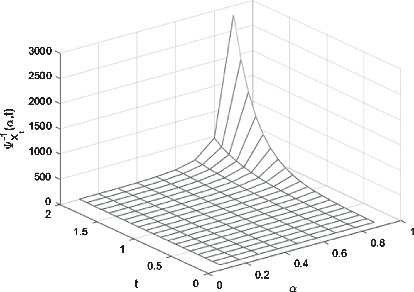
The curve of uncertainty distribution $Ψ_{X_{t}}^{- 1} (α, t)$ .

Example 2. Similar to Example 1, take x₀ = 3, a = 1 and b = 2 in the UDE (5). The inverse uncertainty distribution is $Ψ_{X_{t}}^{- 1} (α, t) = exp (\frac{2 \sqrt{3} t}{π} ln \frac{α}{1 - α} + ln 3 + t) .$ Figure 2 shows the curve of uncertainty distribution $Ψ_{X_{t}}^{- 1} (α, t)$ for α ∈ (0, 1) and 0 < t ≤ 2.

Next we choose 180 observations $Ψ_{X_{t}}^{- 1} (α_{i}, t_{j})$ from the grid intersections of uncertainty distribution $Ψ_{X_{t}}^{- 1} (α, t)$ in Figure 2 for α = 0.1, 0.2, …, 0.9 and t = 0.1, 0.2, …, 2. Obviously, n = 9 and m = 20. Since $\begin{matrix} \sum_{i = 1}^{n} \sum_{j = 1}^{m} (ln Ψ_{X_{t}}^{- 1} (α_{i}, t_{j}) - ln x_{0}) t_{j} = 258.3, \\ \sum_{i = 1}^{n} \sum_{j = 1}^{m} (Φ^{- 1} (α_{i}) t_{j})^{2} = 133.2, \\ \sum_{i = 1}^{n} \sum_{j = 1}^{m} (ln Ψ_{X_{t}}^{- 1} (α_{i}, t_{j}) - ln x_{0}) Φ^{- 1} (α_{i}) t_{j} = 266.3, \end{matrix}$ $\begin{matrix} \sum_{i = 1}^{n} \sum_{j = 1}^{m} Φ^{- 1} (α_{i}) t_{j}^{2} = 9.77 \times 10^{- 15} \end{matrix}$ and $n \sum_{j = 1}^{m} t_{j}^{2} = 258.3$ , by Theorem 3, it is easy to get the IUD-LS estimators of a and b $\begin{matrix} a^{'} & = & \frac{266.3 \times 9.77 \times 10^{- 15} - 258.3 \times 133.2}{(9.77 \times 10^{- 15})^{2} - 258.3 \times 133.2} = 1, \\ b^{'} & = & \frac{258.3 \times 9.77 \times 10^{- 15} - 266.3 \times 258.3}{(9.77 \times 10^{- 15})^{2} - 258.3 \times 133.2} = 2 . \end{matrix}$

4.3 Method III

Consider the UDE (5) with the initial value x₀ (>0). By (3) and Definition 11, we have $\frac{{dX}_{t}^{α}}{dt} = {aX}_{t}^{α} + | b | X_{t}^{α} Φ^{- 1} (α), α \in (0, 1) .$ Without loss of generality, suppose b > 0. Thus, an α-path of the UDE is $X_{t}^{α} = x_{0} exp (at + b Φ^{- 1} (α) t)$ for any α ∈ (0, 1), which is equivalent to the following equation

$ln X_{t}^{α} = ln x_{0} + at + b Φ^{- 1} (α) t, α \in (0, 1) .$ (12)

Let $X_{t_{j}}^{α_{i}}$ be observations of $X_{t}^{α}$ for i = 1, 2, …, n, j = 1, 2, …, m and α_i ∈ (0, 1). Define the error $\begin{matrix} ε_{ij} = ln X_{t_{j}}^{α_{i}} - ln x_{0} - {at}_{j} - b Φ^{- 1} (α_{i}) t_{j} \end{matrix}$ for i = 1, 2, …, n, j = 1, 2, …, m and α_i ∈ (0, 1). In order to obtain the least-square estimators of a and b, we solve the optimization problem $min_{a, b} ε_{ij}^{2}$ (13) $= min_{a, b} \sum_{i = 1}^{n} \sum_{j = 1}^{m} (ln X_{t_{j}}^{α_{i}} - ln x_{0} - {at}_{j} - b Φ^{- 1} (α_{i}) t_{j})^{2} .$

Theorem 4. For UDE (5) with the initial value x₀ (>0), the α-path LS estimators of parameters a and b are $\begin{matrix} \begin{matrix} \tilde{a} = & \frac{\sum_{i = 1}^{n} \sum_{j = 1}^{m} z_{ij} Φ^{- 1} (α_{i}) t_{j} \sum_{i = 1}^{n} \sum_{j = 1}^{m} Φ^{- 1} (α_{i}) t_{j}^{2} - \sum_{i = 1}^{n} \sum_{j = 1}^{m} z_{ij} t_{j} \sum_{i = 1}^{n} \sum_{j = 1}^{m} (Φ^{- 1} (α_{i}) t_{j})^{2}}{(\sum_{i = 1}^{n} \sum_{j = 1}^{m} Φ^{- 1} (α_{i}) t_{j}^{2})^{2} - n \sum_{i = 1}^{n} \sum_{j = 1}^{m} (Φ^{- 1} (α_{i}) t_{j})^{2} \sum_{j = 1}^{m} t_{j}^{2}}, \\ \tilde{b} = & \frac{\sum_{i = 1}^{n} \sum_{j = 1}^{m} z_{ij} t_{j} \sum_{i = 1}^{n} \sum_{j = 1}^{m} Φ^{- 1} (α_{i}) t_{j}^{2} - n \sum_{i = 1}^{n} \sum_{j = 1}^{m} z_{ij} Φ^{- 1} (α_{i}) t_{j} \sum_{j = 1}^{m} t_{j}^{2}}{(\sum_{i = 1}^{n} \sum_{j = 1}^{m} Φ^{- 1} (α_{i}) t_{j}^{2})^{2} - n \sum_{i = 1}^{n} \sum_{j = 1}^{m} (Φ^{- 1} (α_{i}) t_{j})^{2} \sum_{j = 1}^{m} t_{j}^{2}}, \end{matrix} \end{matrix}$ where $z_{ij} = ln X_{t_{j}}^{α_{i}} - ln x_{0}$ and $Φ^{- 1} (α_{i}) = \frac{\sqrt{3}}{π} ln \frac{α_{i}}{1 - α_{i}}$ for i = 1, 2, …, n and j = 1, 2, …, m.

Proof. Similar to Theorem 4. In (8), take $y_{ij} = ln X_{t_{j}}^{α_{i}} - ln x_{0}, u_{ij} = Φ^{- 1} (α_{i}) t_{j},$ and ɛ_ij = ε_ij, t_ij = t_j for i = 1, 2, …, n and j = 1, 2, …, m, and θ = (a, b) ^T. Thus, the optimization problem (10) is formed by $\begin{matrix} min_{a, b} \sum_{i = 1}^{n} \sum_{j = 1}^{m} ɛ_{ij}^{2} = min_{a, b} \sum_{i = 1}^{n} \sum_{j = 1}^{m} (y_{ij} - {at}_{ij} - {bu}_{ij})^{2} . \end{matrix}$ From Lemma 1, the estimators $\tilde{a}$ and $\tilde{b}$ are directly obtained. □

Fig. 3

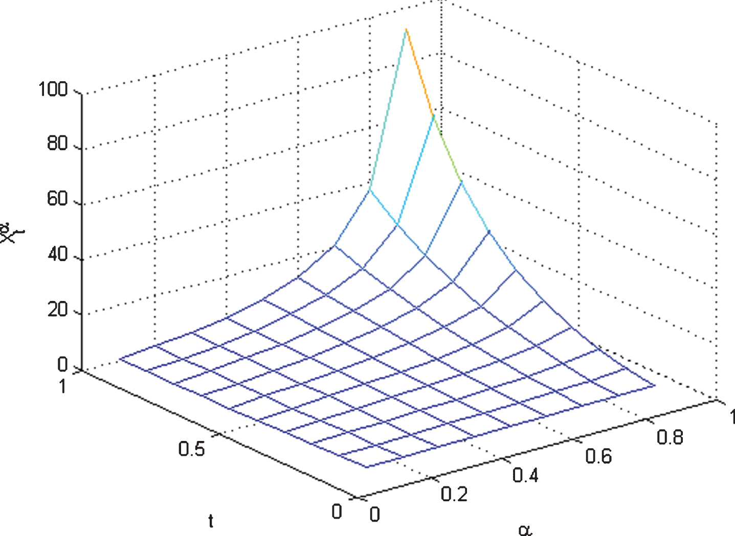
The curve of α-path $X_{t}^{α}$ with x₀ = 3, a = 1 and b = 2.

Example 3. Similar to Example 1, for UDE (5), take x₀ = 3 and a = 1 and b = 2. Thus, the α-path of the UDE is $\begin{matrix} X_{t}^{α} = 3 exp (t + 2 Φ^{- 1} (α) t), α \in (0, 1), \end{matrix}$ Figure 3 shows the curve of α-path $X_{t}^{α}$ .

Next we estimate the parameters a and b of the UDE from the observations $X_{t_{j}}^{α_{i}}$ of $X_{t}^{α}$ , where i = 1, 2, …, n and j = 1, 2, …, m. Take α_i = 0.1, 0.2, …, 0.9 and t_j = 0.1, 0.2, …, 1. Obviously, n = 9 and m = 10. Thus, 90 observations $X_{t_{j}}^{α_{i}}$ are generated from the grid intersections of $X_{t}^{α}$ in Figure 3. By calculation, we have $\begin{matrix} \sum_{i = 1}^{n} \sum_{j = 1}^{m} (ln X_{t_{j}}^{α_{i}} - ln x_{0}) Φ^{- 1} (α_{i}) t_{j} = 35.7253, \\ \sum_{i = 1}^{n} \sum_{j = 1}^{m} Φ^{- 1} (α_{i}) t_{j}^{2} = 8.8818 \times 10^{- 16}, \\ \sum_{i = 1}^{n} \sum_{j = 1}^{m} (ln X_{t_{j}}^{α_{i}} - ln x_{0}) t_{j} = 34.65, \end{matrix}$ $\begin{matrix} \sum_{i = 1}^{n} \sum_{j = 1}^{m} (Φ^{- 1} (α_{i}) t_{j})^{2} = 17.8627 \end{matrix}$ and $n \sum_{j = 1}^{m} t_{j}^{2} = 34.65$ . Based on Theorem 4, we have α-path LS estimators of a and b $\begin{matrix} \tilde{a} & = & \frac{35.7253 \times 8.8818 \times 10^{- 16} - 17.8627 \times 34.65}{(8.8818 \times 10^{- 16})^{2} - 17.8627 \times 34.65} = 1, \\ \tilde{b} & = & \frac{8.8818 \times 10^{- 16} \times 34.65 - 35.7253 \times 34.65}{(8.8818 \times 10^{- 16})^{2} - 17.8627 \times 34.65} = 2 . \end{matrix}$

Examples 1-3 used Methods I, II and III to obtain UD-LS, IUD-LS and α-path LS estimators of a and b, respectively. Since all observations are from the true values of uncertainty distribution, inverse uncertainty distribution and α-path, the corresponding estimators are equal to the true values of a and b.

Fig. 4

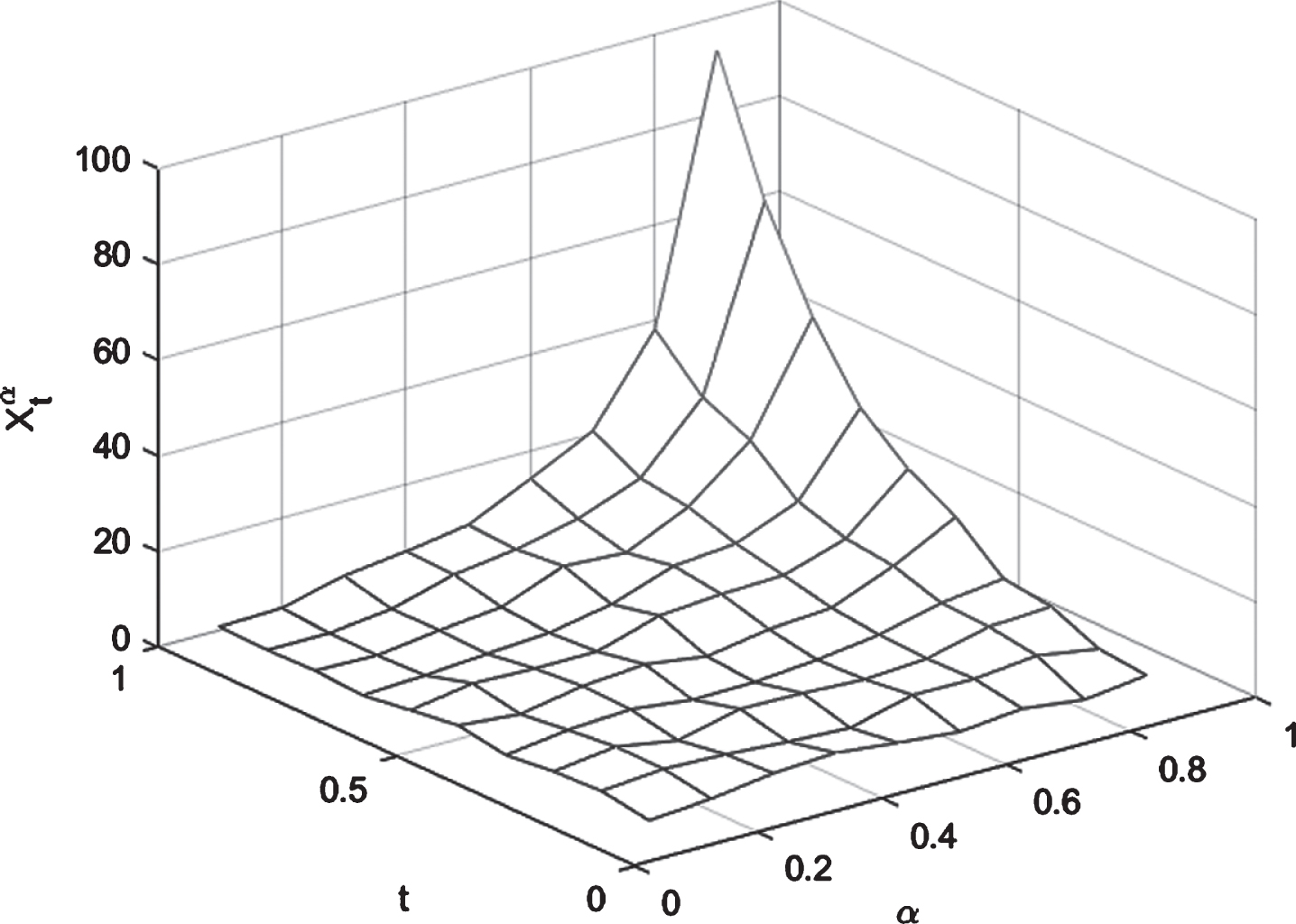
The curve of α-path $X_{t}^{α}$ with noise.

However, in practice, there often exist the errors between estimators and true values of unknown parameters because of observation noise. For instance, Figure 4 shows the curve of an α-path $X_{t}^{α} = x_{0} exp (at + b Φ^{- 1} (α) t)$ with noise, where x₀ = 3. Similar to Example 3, we choose 90 observations of the α-path. From Theorem 4, α-path LS estimators of a and b are ${\tilde{a}}_{1} = 0.7955$ and ${\tilde{b}}_{1} = 2.2853 .$

Furthermore, Methods I, II and III can be extended to estimate multiple unknown parameters of general UDE. Consider the following UDE

$\begin{matrix} {dX}_{t} = f (t, X_{t}; a_{1}, \dots, a_{p}) dt + g (t, X_{t}; b_{1}, \dots, b_{q}) {dC}_{t} \end{matrix}$

with the initial value X₀ = x₀, where a₁, …, a_p and b₁, …, b_q are (p + q) unknown parameters to be estimated. For convenience, let a = (a₁, a₂, …, a_p) and b = (b₁, b₂, …, b_q). Thus, $\begin{matrix} {dX}_{t} = f (t, X_{t}; a) dt + g (t, X_{t}; b) {dC}_{t} \end{matrix}$ Similar to UDE with exponential solutions, we can obtain the corresponding results for estimating a and b.

5 Conclusions

The paper proposed three methods to estimate two unknown parameters a and b of UDE (3). Each method has its own advantage and shortage. Method I is based on the explicit uncertainty distribution of UDE’s solution. Method II is used to solve the estimation problem of UDEs by inverse uncertainty distribution. For Method III, the unknown parameters are estimated by α-path of UDE. In order to illustrate steps of Methods I, II and III, we estimate two unknown parameters a and b of the UDE dX_t = aX_tdt + bX_tdC_t and obtain the corresponding formulas of the estimated values. The numerical simulations reveal that these methods are efficient and practical under certain conditions.

Methods I-III have some limitations. If there are no explicit solutions of a UDE or its corresponding α-path, then we cannot use these method to solve the estimation problem by least-square method. Thus, some novelty methods need to offer a promising solution to overcome the problem, and should be considered in our further work.

Footnotes

Acknowledgments

This research is funded by the National Natural Science Foundation of China (Grant No. 11661076, 11671019) and LMEQF, and the Science and Technology Department of Xinjiang Uygur Autonomous Region (Grant No. 2018Q011).

References

Liu

, Fuzzy process, hybird process and uncertain process, J Uncertain Syst 2 (2008), 3–16.

Chen

and Liu

, Existence and uniqueness theorem for uncertain differential equations, Fuzzy Optim Decis Ma 9(1) (2010), 69–81.

Liu

Y.H.

, An analytic method for solving uncertain differential equations, J Uncertain Syst 6(4) (2012), 244–249.

Yao

, A type of uncertain differential equations with analytic solution, Journal of Uncertainty Analysis and Applications 1 (2013), 1–8.

Liu

, Semi-linear uncertain differential equation with its analytic solution, Information: An International Interdisciplinary Journal 16(2) (2013), 889–894.

Wang

, Analytic solution for a general type of uncertain differential equation, Information: An International Interdisciplinary Journal 16(2) (2013), 1003–1010.

Yao

and Chen

X.W.

, A numerical method for solving uncertain differential equations, J Intell Fuzzy Syst 25(3) (2013), 825–832.

Zhou

and Li

, Analytic solutions of two types of nonlinear uncertain differential equations, J Intell Fuzzy Syst 35 (2018), 2413–2420.

Gao

, Existence and uniqueness theorem on uncertain differential equations with local Lipschitz condition, J Uncertain Syst 6(3) (2012), 223–232.

10.

Liu

, Some research problems in uncertainty theory, J Uncertain Syst 3 (2009), 3–10.

11.

Yao

, Ke

and Sheng

Y.H.

, Stability in mean for uncertain differential equation, Fuzzy Optim Decis Ma 14(3) (2015), 365–379.

12.

Chen

and Gao

, Uncertain term structure model of interest rate, Soft Computing 17(4) (2013), 597–604.

13.

Chen

, American option pricing formula for uncertain financial market, International Journal of Operations Research 8(2) (2011), 32–37.

14.

Yao

, Uncertain contour process and its application in stock model with floating interest rate, Fuzzy Optim Decis Ma 14 (2015), 399–424.

15.

Liu

Y.H.

, Uncertain currency model and currency option pricing, International Journal of Intelligent Systems 30(1) (2015), 40–51.

16.

Zhu

Y.G.

, Uncertain optimal control with application to a portfolio selection model, Cybernetics and Systems 41(7) (2010), 535–547.

17.

Zhu

Y.G.

, Functions of uncertain variables and uncertain programming, J Uncertain Syst 6(4) (2012), 278–288.

18.

, Sheng

, Teng

and Miao

, An uncertain differential equation for SIS epidemic model, J Intell Fuzzy Syst 33 (2017), 2317–2327.

19.

Fang

, Li

, Yang

and Zhou

, Solution and α-path of uncertain SIS epidemic model with standard incidence and demography, J Intell Fuzzy Syst 35 (2018), 927–935.

20.

, Teng

, Du

and Shi

, Comparison of three SIS epidemic models: deterministic, stochastic and uncertain, J Intell Fuzzy Syst 35 (2018), 5785–5796.

21.

, Parameter estimation of simple uncertain differential equations, J Intell Fuzzy Syst 37 (2019), 5363–5372.

22.

Liu

, Uncertainty Theory (2th ed.), Springer, Berlin, (2007).

23.

Liu

, Uncertainty Theory: A Branch of Mathematics for Modeling Human Uncertainty, Springer-Verlag, Berlin, (2010).

24.

Liu

, Uncertainty distribution and independence of uncertain processes, Fuzzy Optim Decis Ma 13(3) (2014), 259–271.