A novel combined model based on VMD and IMODA for wind speed forecasting

Abstract

Wind energy, a highly popular renewable clean energy, has been increasingly valued by the international community and been leaping forward. However, the original wind speed signal characterized by intermittent fluctuations impose heavy burdens on wind speed forecasting of wind farms. This study proposed a wind speed forecasting method by complying with a model integrating the Variational Mode Decomposition (VMD) and the Improved Multi-Objective Dragonfly Optimization Algorithm (IMODA). First, the VMD was adopted to decompose the original wind speed signal, as an attempt to obtain multiple sub-sequences (IMFs) exhibiting stable frequency domain. Second, to simplify the calculation, the sample entropy (SE) was adopted for the sequence recombination, and the respective recombined sub-sequence of the wind speed was forecasted by using four advanced neural networks. Lastly, the IMODA algorithm was adopted to fuse the forecasting results of the neural network, and the results of the optimal wind speed were forecasted. To verify the effectiveness and adaptability of the algorithm, the wind farm data in four different regions were forecasted. As indicated from the results, this algorithm could outperform other algorithms in the comprehensive forecasting accuracy and the model calculation time, and it could be effectively applied for the wind speed forecasting in wind farms.

Keywords

Wind speed forecasting variational mode decomposition IMODA combined model

1 Introduction

As the concept of low-carbon environmental protection is progressively deepened, the development and utilization of wind energy have increasingly aroused the attention of the international community [1]. Accurate wind speed forecasting is capable of reducing the cost of wind power generation operation, rationally arranging dispatching plans of power sector, and laying reliable bases for market bidding, which is of great application significance in economy and engineering [2, 3]. However, the randomness and volatility of wind power increase the difficulty of power dispatching. Currently, domestic and foreign scholars have conducted numerous researches on wind speed forecasting [4], from the perspective of modeling mechanism (e.g., physical methods, statistical methods and intelligent methods) [5 –7]. On the whole, the physical method builds the wind speed mathematical model of the wind turbine’s wheel height by using atmospheric boundary layer dynamics, boundary layer meteorological theory and physical processes. As impacted by the specific geographical conditions and operating conditions of wind turbines, the model exhibits poor versatility [8]. Compared with the physical method, the statistical method exhibits a strong generalization ability, and it is not required to consider the meteorological characteristics around the wind turbine. In [9], an ARIMA with a regression analysis was applied to the practical short-term wind forecasting. Kalman filtering method [10] was adopted to optimize the time series model. It could dynamically modify the weights based on the ARMA model. As indicated from many documents, time series models are only capable of obtaining good forecasting accuracy in short-term scale scenarios [11]. Intelligent learning wind speed forecasting represented by artificial neural networks can approximate any non-linear function by training data to determine the mapping relationship between variables, thereby making the model more flexible [12 –14]. Yin et al. [15] proposed an LSSVM forecasting model, which achieved favorable forecasting results. Xu et al. [16] established an optimized RBF neural network wind speed forecasting model, which has higher forecasting accuracy in short-term wind speed forecasting.

To improve the forecasting accuracy, given the non-stationary characteristics of wind speed, scholars worldwide proposed a method of modal decomposition of the original wind speed, which covered the EMD [17], the EEMD [18], the CEEMDAN [19], the EWT [20] and the VMD [21] and other decomposition methods. Zhang et al. [18] introduced a hybrid model of EEMD and VNN, which could effectively mine the characteristics of power time series and obtain higher forecasting accuracy. Zhang et al. [19] proposed a fully integrated CEEMDAN method based on the EEMD. By adaptively adding positive and negative white noise, the problem that the EMD is prone to modal aliasing is solved, and the iteration is effectively reduced. The number of times increases the reconstruction accuracy, and it is more suitable for analyzing nonlinear signals. Liu et al. [20] used the EWT to decompose the raw wind speed data into several sub-layers, and then they forecasted the low and high frequency wind speed sub-layers by using two different networks. Zhang et al. [21] introduced a forecasting model based on the VMD and the Lorenz disturbance models. The VMD is capable of decomposing the wind speed into several IMFs that fluctuate around the center frequency according to needs. Reducing the effect of uncertain factors helps restore the fluctuation characteristics of the wind speed signal during the forecasting process, while improving the forecasting accuracy. Gu et al. [22] used the VMD and the optimized k-means algorithm [23], and they used radial basis function neural network for the forecasting. This method can effectively improve the regularity of wind speed, as well as the accuracy of wind speed forecasting. Compared with other data processing methods, the VMD more significantly impacts the processing of non-stationary and non-linear signals, and it can more effectively recover the fluctuation characteristics of the signal.

Though the forecasting models based on VMD show that the method has a favorable forecasting effect, the scholars all used a single forecasting model to predict the decomposition sub-sequence of wind speed. However, different frequency domain subsequences exhibit different characteristics. For a single forecasting model, each sub-sequence attribute cannot be satisfied simultaneously. Accordingly, to improve the forecasting accuracy, multiple single neural network forecasting models are used to construct a combined forecasting model to fully exploit the advantages of each forecasting model.

To study combined models, Zhang et al. [24] proposed a combined forecasting model based on the CEEMDAN and the CLSFAP. The method uses the CLSFAP optimization algorithm to find the optimal weight coefficient. Besides, it effectively exploits the advantages of each single forecasting model and greatly improves the forecasting accuracy of the model. Compared with the single neural network model and the benchmark ARIMA model, the combined model exhibits the optimal performance. Xiao et al. [25] adopted the CSO optimization algorithm [26] to determine the optimal weight coefficient of the combined model. Hirose et al. [27] built a k-nearest neighbor algorithm and the MLR combined forecasting model. Since single forecasting models solved the same forecasting problem, their forecasting results were highly correlated, and MLR methods may encounter collinearity or singularity problems, thereby resulting in inaccurate weighting coefficients. In accordance with the theory of non-negative constraints, Niu et al. [28] developed a fully integrated empirical mode decomposition with adaptive noise and a multi-objective grasshopper optimization algorithm. The combined model considers the linear and nonlinear characteristics exhibited by the sequence, successfully addresses the limitations of the single model, and improves the stability and accuracy of the forecasting results. In brief, wind speed forecasting needs accuracy, while requiring the stability of the forecasting algorithm. Single objective optimization algorithms fail to comply with the requirements of accurate and stable wind speed forecasting simultaneously, while multi-objective optimization algorithms can more effectively balance the relationship between objective functions.

To further improve the accuracy of wind speed forecasting, after fully analysis on the advantages and disadvantages of each decomposition method and weight optimization method, a combined wind speed forecasting model based on the VMD and the IMODA was proposed. First, the original wind speed data were decomposed into IMF components of different frequencies by the VMD. In order to simplify the computation, the sample entropy (SE) was adopted to recombine the subsequences, and several components with typical characteristics were obtained. Subsequently, four kinds of neural networks were adopted to build the forecasting models of each component. Lastly, the method of IMODA was adopted to perform weighted fusion of the forecasted results, which synthesized the advantages of each forecasting model to obtain wind speed forecasting results. Furthermore, compared with a variety of forecasting models, the forecasting effect of the model was analyzed.

The main contributions of this paper are listed as follows:

In order to improve the prediction accuracy and reduce the computational complexity, while preserving the fluctuation characteristics of the wind speed series, a parameter-optimised VMD decomposition method is used to decompose the original wind speed to obtain wind speed signals of different frequencies.

In this paper, a multi-objective optimisation algorithm, IMODA, is used to combine the wind speed results predicted by different models in a weighted manner to achieve the optimal prediction results.

The rest of this study is organized as follows: In Section 2, the VMD and the single forecasting models are introduced. In Section 3, the process of the IMODA combination model is described. In Section 4, the forecasting results of the combined model are analyzed and compared. In Section 5, conclusions are drawn. Table 1 lists the abbreviations used in this study.

Table 1
List of Abbreviation

List of Abbreviation

VMD Variational Mode Decomposition

IMODA Improved Multi-Objective Dragonfly Optimization Algorithm

IMF Intrinsic Mode Function

SE Sample Entropy

ARMA Autoregressive Moving Average model

LSSVM Least Squares Support Vector Machine

EMD Empirical Mode Decomposition

EEMD Ensemble Empirical Mode Decomposition

CEEMDAN Complete Ensemble Empirical Mode Decomposition with Adaptive Noise

EWT Empirical wavelet transform

VNN Volterra Neural Network

CLSFAP Flower Pollination Algorithm with Chaos Local Search

ARIMA Autoregressive Integrated Moving Average model

CSO Cuckoo Search Algorithm

MLR Multiple Linear Regression

ADMM Alternate Direction Method of Multipliers

MIGA Multi-island Genetic Algorithm

BP Back Propagation Neural Network

RBF Radial Basis Function Neural Network

GRNN Generalized Regression Neural Network

WNN Wavelet Neural Network

ENN Elman Neural Network

MAE Mean Absolute Error

RMSE Root Mean Squared Error

SSE Sum of Squares due to Error

MAPE Mean Absolute Percent Error

List of Abbreviation
VMD	Variational Mode Decomposition
IMODA	Improved Multi-Objective Dragonfly Optimization Algorithm
IMF	Intrinsic Mode Function
SE	Sample Entropy
ARMA	Autoregressive Moving Average model
LSSVM	Least Squares Support Vector Machine
EMD	Empirical Mode Decomposition
EEMD	Ensemble Empirical Mode Decomposition
CEEMDAN	Complete Ensemble Empirical Mode Decomposition with Adaptive Noise
EWT	Empirical wavelet transform
VNN	Volterra Neural Network
CLSFAP	Flower Pollination Algorithm with Chaos Local Search
ARIMA	Autoregressive Integrated Moving Average model
CSO	Cuckoo Search Algorithm
MLR	Multiple Linear Regression
ADMM	Alternate Direction Method of Multipliers
MIGA	Multi-island Genetic Algorithm
BP	Back Propagation Neural Network
RBF	Radial Basis Function Neural Network
GRNN	Generalized Regression Neural Network
WNN	Wavelet Neural Network
ENN	Elman Neural Network
MAE	Mean Absolute Error
RMSE	Root Mean Squared Error
SSE	Sum of Squares due to Error
MAPE	Mean Absolute Percent Error

2 Related methodology

2.1 Data processing

Data preprocessing: The large amount of raw data collected from wind farms could be very messy, with more or less duplicate data and missing data. Proper data processing of the mentioned anomaly data would effectively improve the forecasting accuracy of the wind speed forecasting model.

Imputation of missing data: In the modeling calculation process, complete wind power data is required to make more accurate wind speed predictions for wind farms. Therefore, the data is checked for completeness before pre-processing the data, and the data is filled in according to the missing types. In this paper, we use the mean fill method [29] to fill the missing data by finding the average of the values before and after the missing values.

Outlier handling: During transmission, abnormal communication lines, poor contact, abnormal acquisition software, and inconsistent computer and acquisition time can cause wind power data outlier situations. In this paper, the DBSCAN algorithm [30] is selected to reject outlier data such as wind turbine shutdown and underpower.

Data normalization: The units of different eigenvalues in the original data were different, and the order of magnitude might vary greatly. If the mentioned data were not processed and analyzed, the feature quantity with small value range would be covered by the considerable features and cannot be exploited. Thus, normalization was performed before the data input model, so all the characteristic variables were normalized to the same order of magnitude, which could simplify the calculation and accelerate the convergence of the model. Lastly, the actual value of the forecasting was calculated through denormalization. The data characteristics were generally normalized to [–1, 1], as expressed in (1): $p_{i}^{'} = \frac{p_{i} - A_{min}}{A_{max} - A_{min}}$ (1)

Where A_max and A_min denote the maximum and minimum values of feature A, respectively, which are p_i eigenvalues, and $p_{i}^{'}$ is the normalized eigenvalue.

2.2 Variational mode decomposition (VMD)

The VMD refers to a novel adaptive signal processing method, exerting a significant processing effect on non-stationary and nonlinear signals [31]. Its adaptability can be manifested in determining the number of modal decompositions of a given sequence by complying with the actual situation. In the searching and solving processes, the optimal center frequency and limited bandwidth of each mode could be adaptively matched to realize the effective separation of IMFs and the frequency domain segmentation of the signal, to obtain the effective decomposition of the given signal. Lastly, the optimal solution of the variational problem was obtained. The VMD is expressed as a constrained variational problem: ${\begin{matrix} {μ_{k}, ω_{k}} = arg min {\sum_{k = 1}^{K} {∥ \partial_{t} [(σ (t) + \frac{i}{π t}) * μ_{k} (t)] e^{- j ω_{k} t} ∥}_{2}^{2}} \\ s . t . \sum_{k = 1}^{K} μ_{k} = f (t) \end{matrix}$ (2)

Where f (t) expresses the original signal; t implicates the time script; K denotes the total number of the modes; μ_k denotes the kth mode; σ (t) represents the Dirac distribution; ω_k is the center frequency. Moreover, the mode with high-order denotes the low-frequency sub-layers.

To convert the mentioned optimization problem into an unconstrained one, the penalty term and Lagrangian multipliers were employed, which is expressed as: $\begin{matrix} L {{μ_{k}}, {ω_{k}}, λ} = α \sum_{k = 1}^{K} {∥ \partial_{t} [(σ (t) + \frac{i}{π t}) * μ_{k} (t)] e^{- j ω_{k} t} ∥}_{2}^{2} \\ + {∥ f (t) - \sum_{k = 1}^{K} μ_{k} (t) ∥}_{2}^{2} + 〈 λ (t), f (t) - \sum_{k = 1}^{K} μ_{k} (t) 〉 \end{matrix}$ (3)

Where α is the balancing parameter of the needed data fidelity constraint.

The mentioned variation problem was solved by using the ADMM (Alternate Direction Method of Multipliers), which could determine the saddle point of the Lagrangian expression by updating: ${\overset{⌢}{μ}}_{k}^{n + 1} (ω) = \frac{\overset{⌢}{f} (ω) - \sum_{i \neq k} μ_{i}^{⌢} (ω) + \frac{\overset{⌢}{λ} (ω)}{2}}{1 + 2 α (ω - ω_{k})}$ (4) $ω_{k}^{n + 1} = \frac{\int_{0}^{\infty} ω {| μ_{k}^{⌢} (ω) |}^{2} d ω}{\int_{0}^{\infty} {| μ_{k}^{⌢} (ω) |}^{2} d ω}$ (5) ${\overset{⌢}{λ}}^{n + 1} (ω) = {\overset{⌢}{λ}}^{n} (ω) + τ (\overset{⌢}{f} (ω) - \sum_{k = 1}^{K} {\overset{⌢}{μ}}_{k}^{n + 1} (ω))$ (6)

According to the VMD theory, when using the VMD algorithm to process signals, the modal component k and the penalty parameter α should be initialized, and different parameter settings can lead to different VMD results. Based on the parameters set manually, the decomposition result will be uncertain and random. Accordingly, optimization algorithms should be used to find the optimal parameter combination. In the literature [32], Liang et al. adopted the MIGA to optimize VMD parameters and achieved good decomposition results in bearing vibration signals. This study applied it to the decomposition of wind speed signal. The optimized parameter values are α=2000 and k = 10. The decomposition results are presented in Fig. 1.

Fig. 1

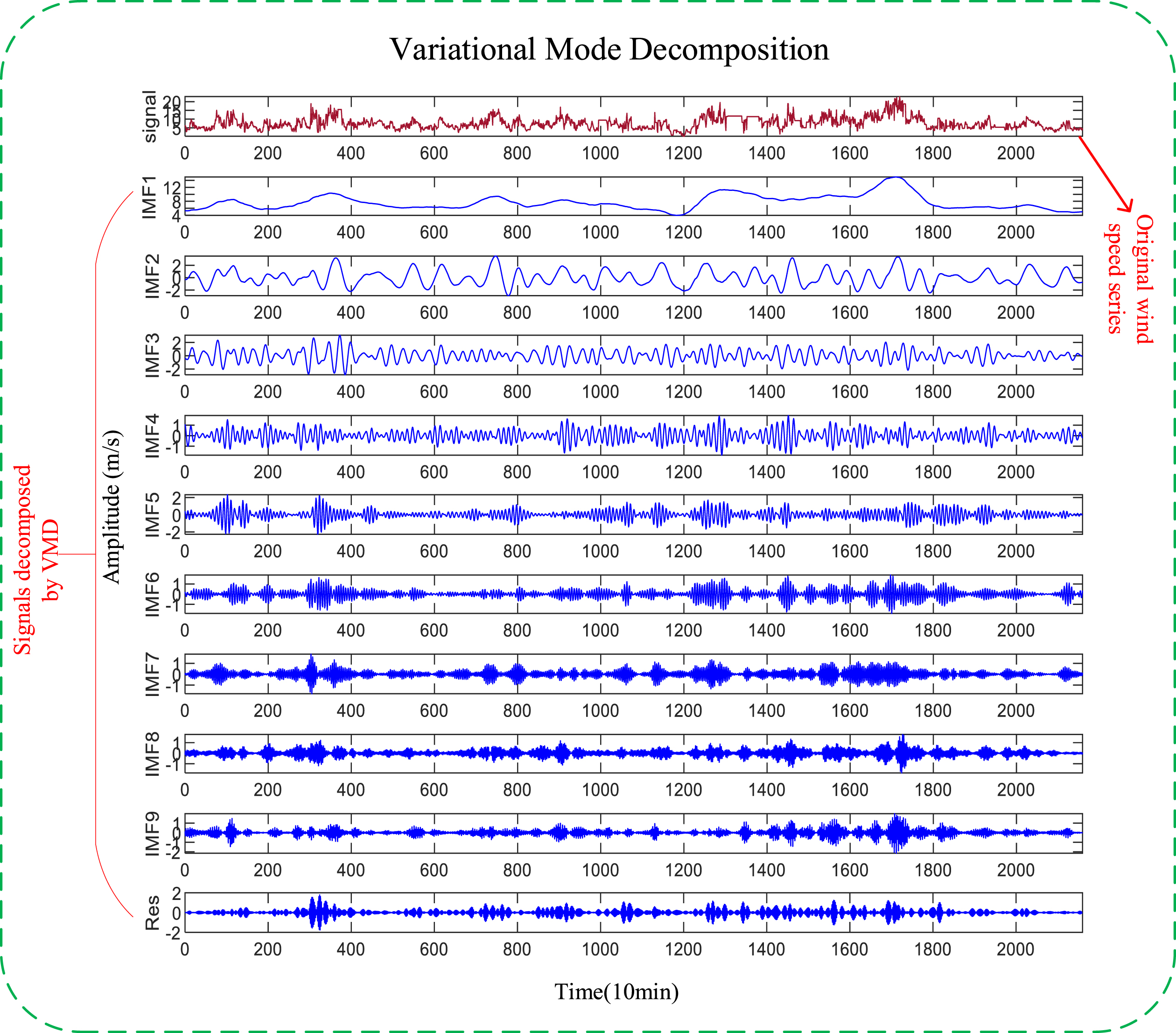
The IMFs of the VMD method.

2.3 Sample entropy

For the multiple IMF components decomposed by the VMD, if the prediction model is established separately, the calculation amount will increase, and the correlation between the individual components will be ignored. To simplify the calculation, the characteristics of the similar sequences were highlighted, and the components with correlation were recombined. The sample entropy in 2004 refers to an algorithm proposed by Richman and collaborators to improve the time series complexity for the approximate entropy improvement [33]. The smaller the value of the sample entropy, the lower the complexity of the sequence would be. Conversely, the sequence would be more complex. Given this, the sub-sequence was processed by sample entropy.

The sample entropy is represented by SampEn (m, v, N), where N is the data length, m denotes the dimension, and v is the tolerance. For a given vector X(i), count the number of j(1≤j≤N-m,j≠i) with distance less than tolerance v between X(i) and X(j),denoted as B(v). With N as a finite value, the sample entropy estimate is expressed as: $SampEn (m, v, N) = - ln \frac{B^{m + 1} (v)}{B^{m} (v)}$ (7)

Though the sample entropy was related to the values of m and v, the sample entropy exhibits high consistency, and the entropy value change trend was not affected by m and v. Typically, m was 1 or 2, and v was 0.1 to 0.25 SD, where SD denotes the standard deviation of the sequence. In this study, m = 1, v = 0.15SD, as shown in Fig. 2, the sample entropy value distribution of the sequence. The sample entropy values of some subsequences were relatively close, and the IMF components were regrouped. The larger the sample entropy value, the higher the complexity would be. The complexity of IMF2 and IMF3 should be separately modeled. The entropy values of IMF1, IMF4 and IMF5 were close to each other and should be merged into one subsequence for modeling. The complexity of IMF6 IMF10 was combined into one subsequence for modeling. Reorganized IMF1 IMF10 into IMF1’, IMF2’, IMF3’, IMF4’.

Fig. 2

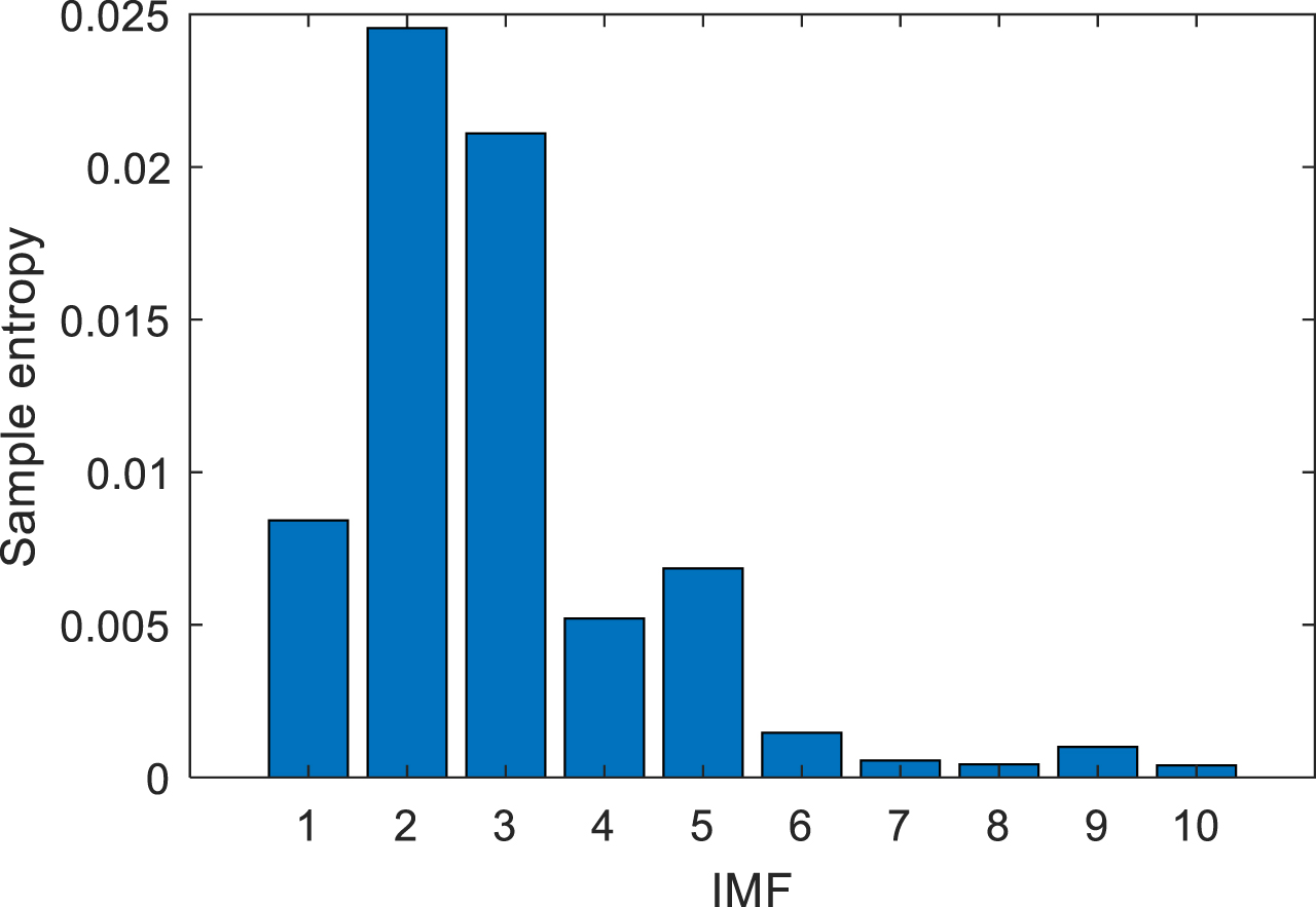
The SampEn of the IMFs.

2.4 Single forecasting model

(1) BP neural network

The BP neural network refers to a multi-layer forward neural network based on the gradient descent method [34]. The learning process could roughly have two parts, i.e., forward calculation and back propagation. The back propagation falls to two stages of updating and learning. $w_{ij} (t) = w_{ij} (t - 1) - Δ w_{ij} (t)$ (8) $Δ w_{ij} (t) = η \partial E / \partial Δ w_{ij} (t - 1) + α \cdot Δ w_{ij} (t - 1)$ (9)

Where w_ij denotes the weight between nodes i and j; η is the learning speed; α expresses the impulse parameter; t is the current number of iterations; E is the error hypersurface.

(2) RBF neural network

The RBF neural network structure comprises an input layer, an implicit layer and an output layer, which is a typical feedforward neural network [35]. Set the input of the RBF neural network as X = [x₁, x₂, ⋯ , x_p], and then the function of the h-th hidden node is set as follows; $φ_{h} (x_{p}) = exp (- \frac{{∥ x_{p} - c_{h} ∥}^{2}}{σ_{h}})$ (10)

Where c_h and σ_h respectively represent the center and width of the h-th hidden layer node kernel function; ∥· ∥ is adopted to calculate the Euclidean distance.

The output of the network to the p-th sample is: $y_{p} = \sum_{h = 1}^{H} ω_{h} φ_{h} (x_{p})$ (11)

Where ω_h denotes the connection weight of the h-th hidden node and the output node.

(3) Wavelet neural network

Wavelet neural network combines wavelet transform and artificial neural networks [36]. It comprises the time domain localization of wavelet analysis and the self-learning ability of artificial neural networks. The mother wave function can represent a traditional sigmoid function, as more accurately reflected in time series and time domain distributions of different scales. A set of mother waves can be approximated by: $y_{k} (x) = \sum_{j = 1}^{J} w_{ji} φ (\frac{X_{j} - b_{j}}{a_{j}}), (k = 1, \dots K)$ (12)

Where $X_{J} = \sum_{i = 1}^{I} w_{ji} x_{i}, (j = 1, . . . J)$ ; φ (·) is the WNN base function; a_j, b_j (j = 1, . . . J) is the expansion and translation parameters of the wavelet function at the hidden node j, respectively. In this study, the basic mother wave function took the real part: $φ (t) = \cos (1.75 t) \exp (- \frac{t^{2}}{2})$ (13)

(4) Generalized Regression Neural Network

GRNNs refer to an important branch of radial basis neural networks [37]. They mainly consist of four parts, i.e., an input layer, a mode layer, a summation layer and an output layer. The algorithm exhibits a strong nonlinear mapping capability and a flexible network structure, as well as high fault tolerance and robustness, and it is suitable for solving various nonlinear problems.

Mode layer: The number of neurons in the pattern layer is equated with that of learning samples, and each neuron corresponds to a different sample. There is a nonlinear transformation transforming the input space into a pattern space. The relationship between the input neurons and the pattern layer can be stored in the respective neuron of the layer.

Summing layer: The summation layer employs two types of neurons for summation, i.e., simple summation s_s and weighted summation s_w. Subsequently, the summation layer is transferred to the output layer.

The input and output nodes of the four neural networks are set to 5 and 1. The parameter settings for the four neural networks are listed in Table 2.

Table 2

Experiment parameters of the four ANN’s

Model	Experimental parameters	Default value
BPNN	The learning velocity	0.01
	The maximum number of trainings	1000
	Training requirements precision	0.00004
RBF	Spread of radial basis function	0.5
	Training requirements precision	0.00004
WNN	Learning rate	0.1
	Training requirements precision	0.00004
GRNN	Spread of radial basis functions	0.1

3 Combined model based on IMODA

In ordinary combined forecasting, it is usually only the use of simple optimization algorithms to combine the forecasting models with the forecasting accuracy as the objective function, and the stability of the forecasting is ignored [28]. For combined models, the weights should be scientifically and comprehensively determined to acquire accurate and stable forecasting results. Thus, the IMODA was adopted to determine the weights of the four forecasting models to achieve the optimal forecasting effect.

3.1 Improved multi-objective dragonfly optimization algorithm

The multi-objective Dragonfly algorithm is a novel swarm intelligence algorithm proposed by Mirjalili of Griffith University in Australia in recent years [38]. Such an algorithm is primarily inspired by the static and dynamic group behavior of dragonflies, which indicates that the group preys, and the dynamic group behavior means that the group migrates. The mentioned two cluster behaviors can be equivalent to the searching and development of the optimization algorithm. In the algorithm, a mathematical model is built to simulate the group behavior of dragonflies. Dragonfly algorithm exhibits the advantages of its high accuracy, fast convergence and good stability. However, consistent with other population-based heuristic algorithms, the basic multi-objective Dragonfly algorithm is prone to fall into local optimum and uneven distribution of non-inferior solutions. In this study, the IMODA was proposed. The hybrid mutation operator was introduced into the multi-objective dragonfly optimization algorithm to increase the diversity of the population and reduce the possibility that the population falls into the local optimum. Subsequently, the dynamic file maintenance strategy based on the crowding distance was adopted to make the Pareto solution set distributed more effectively [39].

3.1.1 MODA

In the MODA, there are five main factors of the population, i.e., separation, alignment, aggregation, food attraction and natural enemy dispersion. The mathematical models of the mentioned five factors are presented below:

Separation is the avoidance of collisions between individuals and other nearby individuals: $S_{i} = - \sum_{j = 1}^{N} X - X_{j}$ (14)

Where X represents the location of the current individual, X_j denotes the location of the j-th neighboring individual, and N expresses the number of individuals.

Alignment represents to the degree to which an individual and other nearby individual have the same speed: $A_{i} = \frac{\sum_{j = 1}^{N} V_{j}}{N}$ (15)

Where V_j expresses the speed of the j-th individual nearby.

The degree of aggregation refers to the tendency of the individual to approach the center of mass nearby: $C_{i} = \frac{\sum_{j = 1}^{N} X_{j}}{N} - X$ (16)

Where X represents the position of the individual; N denotes the number of nearby individuals.

Food attraction refers to the tendency of individuals to approach food: $F_{i} = X^{+} - X$ (17)

Where X is the position of the current individual; X⁺ expresses the position of the food.

The dispersal of natural enemies is the degree to which the individual is far away from the natural enemies in nature: $E_{i} = X^{-} + X$ (18)

Where X denotes the current personal position; X^- represents the position of natural enemies.

Mathematical model of step vector update: $Δ X_{t + 1} = ({sS}_{i} + {aA}_{i} + {cC}_{i} + {fF}_{i} + {eE}_{i}) + ω Δ X_{t}$ (19)

Where s represents the separation coefficient; a is the alignment coefficient; c is the aggregation coefficient; f is the food attraction coefficient; e is the natural enemy dispersal coefficient; ω is the inertia coefficient; t is the iteration count subscript.

Mathematical model of position vector update: $X_{t + 1} = X_{t} + Δ X_{t + 1}$ (20)

Where t denotes the current number of iterations.

3.1.2 Hybrid mutation operator

By applying the mutation operator [40] to the optimization algorithm, the algorithm’s exploration ability can be improved. Since uniform mutation can cause degradation, this study employed a mixed mutation operator based on random average mutation and Gaussian mutation, and the mutation method of selected individuals was calculated as: $x_{t, d}^{'} = x_{\min, d}^{'} + α (x_{\max, d}^{'} - x_{\min, d}^{'})$ (21) $x_{t, d}^{'} = x_{t, d}^{'} (1 + 0.5 N (0, 1))$ (22)

Where t is the current iteration number; α represents the random number on [0, 1]; x_t,d denotes the position before the individual mutation; x_max,d and x_min,dare the maximum and minimum values of the individual on the d-th dimension, respectively; $x_{\max, d}^{'}$ and $x_{\min, d}^{'}$ are the variation values of the maximum value and minimum value of the individual on the d-th dimension, respectively.

At the early stage of the algorithm, a larger mutation probability increased the population diversity and helped find more non-inferior solutions. At the subsequent stage of the algorithm, a smaller value contributed to the convergence of the algorithm. The variation probability was applied to the variation range, so the variation range decreased with the increase in the number of iterations. At the early stage of the algorithm, the entire search space could be optimized, and the smaller variation range at the subsequent stage was to ensure the development ability of the algorithm in the subsequent iteration.

3.1.3 Dynamic maintenance strategy of external archives based on crowded distance

In the algorithm, the crowding distance was adopted to estimate the density of the non-dominated solutions, thereby keeping the non-dominated solutions distributed effectively [41]. In this study, a dynamic maintenance strategy based on crowding distance was adopted to maintain the diversity of Pareto solution sets. The congestion distance component was calculated as: $I_{P (x, k) - 1} = | f_{P (x, k) + 1} - f_{P (x, k) - 2} |$ (23) $I_{P (x, k) + 1} = | f_{P (x, k) + 2} - f_{P (x, k) - 1} |$ (24)

Where p (x, k) represents the location information of the optimal solution x on the k-th objective dimension; f_p(x,k) is the corresponding objective function value.

In the dynamic maintenance, only the optimal solution with the smallest congestion distance was deleted each time, and the optimal solution affected in each target dimension was yielded according to the location information of the deleted optimal solution. The congestion distance component of the affected optimal solution was recalculated, and its congestion distance was updated. Next, the Pareto optimal set was maintained based on the novel crowding distance, as an attempt to avoid deleting individuals in numerous dense areas at one time. Accordingly, the size of Pareto optimal solution was continuously recycled to reach the maximum capacity of external files.

3.2 The basic structure and specific steps of the combined model

As indicated from the results of VMD decomposition, different IMF components exhibited different characteristics, and a single forecasting model failed to satisfy all the properties of IMF’ components. A combination method with IMODA was proposed for mentioned problem. The specific steps are presented as follows:

Step 1: The original wind speed signal was decomposed by the VMD with MIGA optimized parameters to obtain several IMFs with different frequencies. Then, the sample entropy of each IMF was calculated, and the subsequence was recombined according to the sample entropy value, as an attempt to obtain four typical components, i.e., IMF1’, IMF2’, IMF3’ and IMF4’.

Step 2: The four reconstructed signals IMF1’, IMF2’, IMF3’ and IMF4’ were forecasted by using four models of BP, RBF, WNN and GRNN to obtain four forecasting values with different accuracies, respectively. Next, the four forecasted values of each reconstructed signal were put into IMODA algorithm respectively, and the optimal weights w₁, w₂, w₃ and w₄ of the four forecasted values were calculated by IMODA with $min_{MAPE}$ and $min_{std}$ as the objective functions. Lastly, the forecasting results of several models were weighted and summed to obtain the optimal forecasting results of each reconstructed signal. P_model (Model=’BPNN’, ‘RBFNN’, ‘WNN’, ‘GRNN’) was assumed as the forecasting result of the four methods for each IMF’. Subsequently, the combined weighted output of each IMF’ is expressed as:

$\begin{matrix} {output}_{IMODA}^{{IMF}_{S}} = w_{1} \times P_{model 1} + w_{2} \times P_{model 2} \\ + w_{3} \times P_{model 3} + w_{4} \times P_{model 4} \end{matrix}$ (25)

Where w_i (i = 1, 2, . . . , N) is the weight coefficient of the model N.

Step 3: The optimal forecasting results of the four reconstructed signals were obtained by IMODA optimization, and the final wind speed forecasting results could be obtained by summing the forecasting results of the four components.

$\begin{matrix} {output}_{wind} = {output}_{IMODA}^{{IMF}_{1}} + {output}_{IMODA}^{{IMF}_{2}} \\ + {output}_{IMODA}^{{IMF}_{3}} + {output}_{IMODA}^{{IMF}_{4}} \end{matrix}$ (26)

The specific steps are illustrated in Fig. 3.

Fig. 3

The procedure of the proposed combined model.

4 Experiments and analysis

4.1 Data description

In this study, based on the wind power data of four wind farms in Xin Yu, Dong Tuanbao, Liu Jiazhuang and Hai Xing (hereinafter referred to as site 1, site 2, site 3 and site 4, respectively) in 2017, the forecasting effect was evaluated, as presented in Fig. 4. Moreover, the data were used to verify whether the proposed model is suitable for different occasions. From January 1, 2017 to January 15, 2017, wind speed data was sampled every 10 minutes, 2160 samples from 15 days were selected, and 288 sample data from the next two days were adopted to propose a combined forecasting model performance testing. The forecasting results are presented in Fig. 4. To test the proposed combined forecasting model, four evaluation indicators were used to compare the combined model with other single models. The mean absolute error (MAE), root mean squared error (RMSE), sum of squares due to error (SSE), mean absolute percent error (MAPE) calculation is listed in Table 3.

Fig. 4

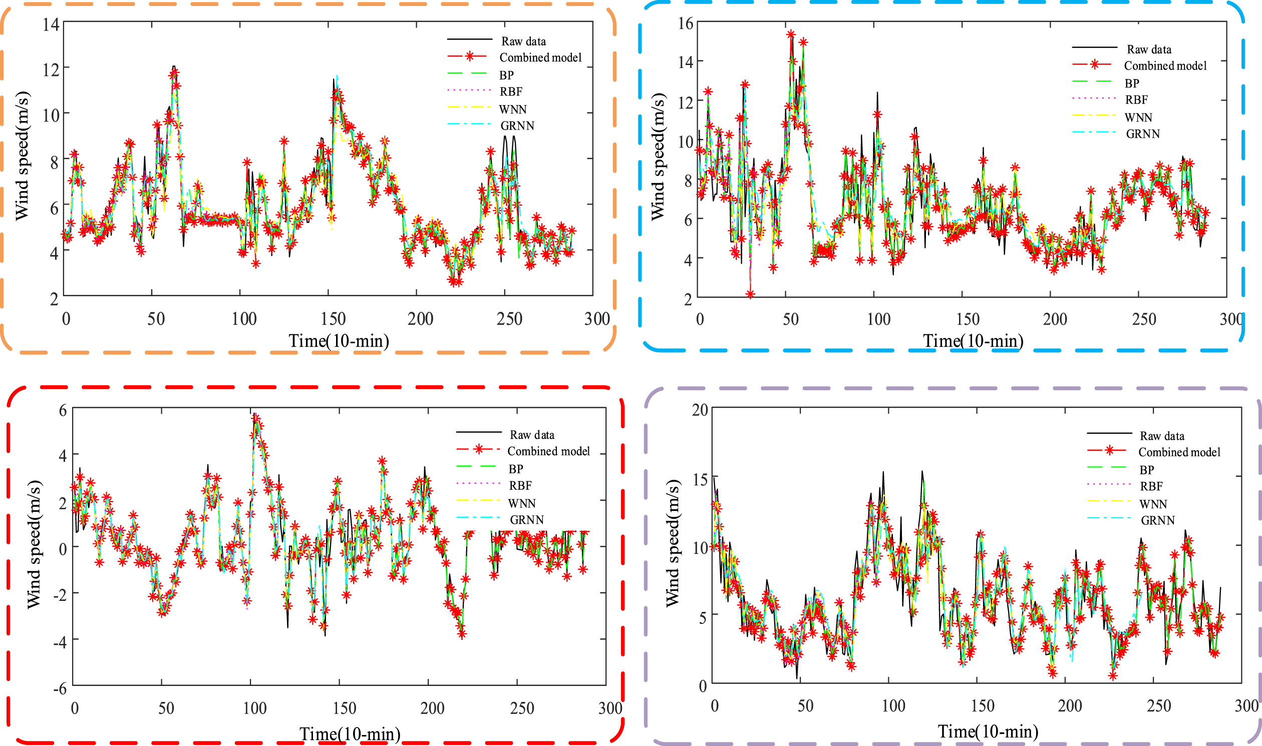
Forecasting results of the combined model and individual models.

Table 3

The four evaluation rules

Metric	Equation	Definition
MAE	$MAE = \frac{1}{N} \sum_{n = 1}^{N} \| y_{n} - {\hat{y}}_{n} \|$	The average absolute forecast error of n times forecast results
RMSE	$RMSE = {(\frac{1}{N} \sum_{n = 1}^{N} {(y_{n} - {\hat{y}}_{n})}^{2})}^{1 / 2}$	The root mean squared forecast error
SSE	$SSE = \sum_{n - 1}^{N} {(y_{n} - {\hat{y}}_{n})}^{2}$	The square sum of the error
MAPE	$MAPE = \frac{1}{N} \sum_{n = 1}^{N} \| \frac{y_{n} - {\hat{y}}_{n}}{y_{n}} \| \times 100 %$	The average of absolute error

4.2 Comparison with classic individual models

Different neural network forecasting models have different forecasting accuracy and forecasting stability for different wind speed series. To improve the accuracy and adaptability of the model, a number of classic neural networks were selected for comparative experiments, including BP, RBF, GRNN, WNN and ENN five typical forecasting models. The forecasting results of the five models in the four wind fields are listed in Table 4.

Table 4
The evaluation among the five ANNS models in four sites

Site Evaluation criteria Models

BPNN RBFNN WNN GRNN ENN

Xin Yu MAE(m/s) 0.7954 0.8323 1.1645 1.1107 1.1738

RMSE(m/s) 1.0516 1.1177 1.4861 1.4963 1.5671

SSE(m/s) 584.2369 595.2365 602.2146 623.1589 641.7326

MAPE(%) 14.3095 13.4813 15.3145 15.5635 16.3725

Dong Tuanbao MAE(m/s) 0.9036 0.9713 1.1912 1.3535 1.3895

RMSE(m/s) 1.3901 1.4271 1.6122 1.6521 1.7344

SSE(m/s) 652.1245 689.5412 695.2155 704.2568 721.3542

MAPE(%) 17.4021 17.5745 15.5514 18.5841 18.9673

Liu Jiazhuang MAE(m/s) 0.8119 0.9013 1.0258 1.1254 1.1344

RMSE(m/s) 1.0542 1.1250 1.2586 1.3201 1.3679

SSE(m/s) 352.1020 385.1026 412.0150 456.2510 449.3729

MAPE(%) 11.4730 12.0252 12.5874 13.1562 12.7931

HaiXing MAE(m/s) 0.8145 0.8211 0.9355 0.9592 0.9475

RMSE(m/s) 1.5625 1.6841 1.7717 1.7820 1.8021

SSE(m/s) 421.2510 452.2103 482.1520 492.1500 516.3789

MAPE(%) 14.6510 14.8554 15.1252 15.5621 15.8973

Site	Evaluation criteria	Models
Xin Yu	MAE(m/s)	0.7954	0.8323	1.1645	1.1107	1.1738
	RMSE(m/s)	1.0516	1.1177	1.4861	1.4963	1.5671
	SSE(m/s)	584.2369	595.2365	602.2146	623.1589	641.7326
	MAPE(%)	14.3095	13.4813	15.3145	15.5635	16.3725
Dong Tuanbao	MAE(m/s)	0.9036	0.9713	1.1912	1.3535	1.3895
	RMSE(m/s)	1.3901	1.4271	1.6122	1.6521	1.7344
	SSE(m/s)	652.1245	689.5412	695.2155	704.2568	721.3542
	MAPE(%)	17.4021	17.5745	15.5514	18.5841	18.9673
Liu Jiazhuang	MAE(m/s)	0.8119	0.9013	1.0258	1.1254	1.1344
	RMSE(m/s)	1.0542	1.1250	1.2586	1.3201	1.3679
	SSE(m/s)	352.1020	385.1026	412.0150	456.2510	449.3729
	MAPE(%)	11.4730	12.0252	12.5874	13.1562	12.7931
HaiXing	MAE(m/s)	0.8145	0.8211	0.9355	0.9592	0.9475
	RMSE(m/s)	1.5625	1.6841	1.7717	1.7820	1.8021
	SSE(m/s)	421.2510	452.2103	482.1520	492.1500	516.3789
	MAPE(%)	14.6510	14.8554	15.1252	15.5621	15.8973

With site 1 as an example, the MAPE values of each forecasting model reached 14.3095%, 13.4813%, 15.3145%, 15.5635%, and 16.3725%, respectively. The RBF neural network exhibited the highest forecasting accuracy, and the ENN exhibited the worst forecasting accuracy. In station 2, the RMSE values of the forecasting models are 1.3901, 1.4271, 1.6122, 1.6521, and 1.7344, respectively. It can be seen that BP and RBF have the highest forecasting accuracy, followed by WNN and GRNN, and ENN has the largest error. In site 3, the MAE values of each model are 0.8119, 0.9013, 1.0258, 1.1254, and 1.1344, respectively, and the forecasting accuracy of the BP neural network is the highest. In site 4, the SSEs of the forecasting models were 421.2501, 452.2103, 482.1520, 492.1500, 516.3789, respectively. The BP and the RBF were suggested to exhibit the best stability in the forecasting of this site, and the GRNN and the ENN exhibited relatively poor forecasting stability. As revealed from the experimental results of the mentioned four sites, the forecasting effects of the BP and the RBF were relatively good, and the forecasting stability of the GRNN and the ENN was poor, whereas the average forecasting ability of the GRNN was higher than the ENN.

When multiple neural networks were weighted and combined, the literature [42] proved that on average, the more single forecasting models combined, the higher the forecasting accuracy would be. However, if all wind farms were combined with more neural networks, the forecasting results would not be better. With the increase in predictive neural networks, the calculation time of the combined model would also increase significantly. This study selected three (BP, RBF and WNN), four (BP, RBF, WNN and GRNN), and five (BP, RBF, WNN, GRNN and ENN) neural networks with the best forecasting results to conduct the combined comparison experiments. According to the comparison experiments, the average forecasting indicators of the combined model in the four wind fields are listed in Table 5. From the experimental results, the SSE values of the combined model combining three, four, and five neural networks were 194.5399, 72.8405, and 68.3770, respectively. It can be seen that the forecasting accuracy of the five neural networks was the highest, and the average SSE value of the four neural networks was much higher than the average SSE value of the three neural networks. However, the SSE value based on five neural networks after joining the ENN network was only 4.4635 higher than the SSE value based on four neural networks, while the model calculation time increased significantly. Accordingly, when the forecasting effect of the model was nearly the same, it could be more practical to choose a forecasting model combining four neural networks with a faster calculation speed.

Table 5

Evaluation index of combined model of different number of ANNs

	MAE	RMSE	SSE	MAPE
BP, RBF, and WNN	0.4586	0.5367	194.5399	7.2583
BP, RBF, WNN and GRNN	0.2235	0.2981	72.8405	4.6602
BP, RBF, WNN GRNN and WNN	0.2107	0.2726	68.3770	4.3795

In this study, four neural networks BP, RBF, WNN, and GRNN with relatively favorable forecasting effects are selected for model combination. The comparison of the forecasting results of a single neural network and the combined model is shown in Fig. 4.

4.3 Comparison of IMFs with different complexity

The purpose of this experiment is to verify the forecasting effectiveness of the forecasting model proposed in this study for signals of different complexity. The BPNN, RBFNN, WNN and GRNN forecasting models based on the IMODA combination model were used to predict the IMF’ sequence, i.e., IMF1’, IMF2’, IMF3’ and IMF4’ obtained by reconstructing IMF sequence in Section 2.3.

The SSE acted as the evaluation index to evaluate the performance of the model. The forecasting results of the single model and the combined model are presented in Fig. 5 and Table 6. For site 1, by comparing the SSE values of four IMF’ sequence, it can be seen that the higher the complexity of the sequence, the greater the forecasting error. However, the SSE values of the combined model proposed in this study were the lowest among the four sequences with different complexity, and the combined model can allocate weights reasonably according to the prediction effects of different prediction models to achieve the best prediction effect. It was therefore indicated that the proposed model could predict the signals with different complexity effectively. Furthermore, to verify the adaptability of the model, four sites were forecasted in total, and the forecasting results of site 2, site 3 and site 4 were as expected.

Fig. 5

The SSE comparison among combined model and single models by forecasting each IMF’s.

Table 6

The forecasting results of the models in four sites

Site	Models	IMF1’		IMF2’		IMF3’		IMF4’
		Weights	SSE	Weight	SSE	Weight	SSE	Weight	SSE
Xinyu	BPNN	0.3891	72.0046	0..8820	133.8440	0.9438	105.8133	0.9121	3.1562
	RBFNN	0.3592	69.5691	0.0410	163.0975	0.0363	131.6729	0.0237	13.7374
	WNN	0.0249	70.8042	0.0034	127.9284	0.0121	121.6276	0.0014	14.7524
	GRNN	0.2268	83.6110	0.0736	109.1826	0.0078	103.0382	0.0628	14.9362
	Combined model	–	55.6398	–	85.3625	–	82.5648	–	1.2152
Dong Tuanbao	BPNN	0.4862	160.7868	0.3695	12.8609	0.6062	13.9115	0.5423	0.3495
	RBFNN	0.2115	161.0259	0.3215	21.4154	0.0985	21.6852	0.0425	0.1467
	WNN	0.1131	175.5364	0.2895	27.9828	0.2032	26.9003	0.3520	0.6815
	GRNN	0.1892	188.1383	0.0195	28.1110	0.0921	27.3155	0.0632	0.1483
	Combined model	–	142.2156	–	8.3652	–	8.3695	–	0.0025
Liu Jiazhuang	BPNN	0.0256	121.3659	0.4520	80.3652	0.8520	45.1256	0.5213	2.2635
	RBFNN	0.4523	136.2598	0.3212	81.1256	0.0211	48.2569	0.2216	2.6985
	WNN	0.3652	142.3612	0.1523	83.2589	0.0612	52.2369	0.0030	5.2698
	GRNN	0.1569	148.2356	0.0745	86.2514	0.0657	52.3698	0.2541	7.2563
	Combined model	–	100.3652	–	72.2356	–	36.2599	–	1.2368
HaiXing	BPNN	0.2015	132.2560	0.5412	74.5623	0.2585	54.2596	0.4789	2.1563
	RBFNN	0.3965	89.3651	0.2256	78.2564	0.5623	56.2345	0.3120	2.3695
	WNN	0.0211	139.2562	0.2121	85.3269	0.1780	59.2561	0.1230	1.5629
	GRNN	0.3809	142.2650	0.0211	89.2356	0.0012	63.2159	0.0861	2.1589
	Combined model	–	78.6582	–	69.3254	–	46.2589	–	1.2036

4.4 Comparison of forecasting results of combined models

4.4.1 Comparison with other VMD-based models

In this experiment, four VMD-based forecasting models were used to compare with the proposed combined model. VMD-based forecasting models include the VMD-BPNN, the VMD-RBFNN, the VMD-WNN and the VMD-GRNN, each model used to predict all IMFs decomposed by the VMD. The forecasting results of the combined model and comparison with other models are presented in Fig. 6 and Table 7.

Fig. 6

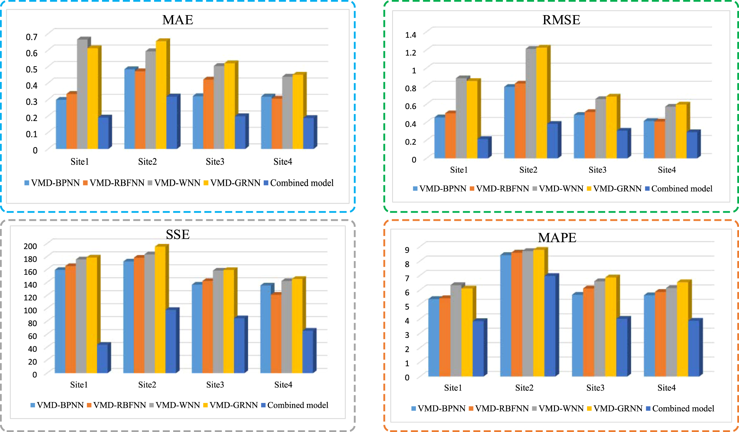
Evaluation index of four wind farms.

Table 7

The evaluation among the combined model and four VMD-ANNS models in four sites

Site	Evaluation criteria	Models
		Combined model	VMD-BPNN	VMD-RBFNN	VMD-WNN	VMD-GRNN
Xin Yu	MAE(m/s)	0.1903	0.2981	0.3333	0.6642	0.6108
	RMSE(m/s)	0.2137	0.4536	0.4987	0.8868	0.8563
	SSE(m/s)	43.7549	159.3652	165.2587	175.5872	178.5421
	MAPE(%)	3.8322	5.3595	5.4203	6.3256	6.0935
Dong Tuanbao	MAE(m/s)	0.3179	0.4836	0.4713	0.5925	0.6535
	RMSE(m/s)	0.3824	0.7909	0.8279	1.2122	1.2255
	SSE(m/s)	97.4762	172.3698	178.2100	183.2596	195.2354
	MAPE(%)	6.9573	8.4053	8.5717	8.6813	8.7652
Liu Jiazhuang	MAE(m/s)	0.1983	0.3199	0.4209	0.5035	0.5201
	RMSE(m/s)	0.3063	0.4804	0.5129	0.6567	0.6842
	SSE(m/s)	84.6546	136.5280	142.1258	158.3020	159.2014
	MAPE(%)	3.9941	5.6574	6.0992	6.5874	6.8523
Hai Xing	MAE(m/s)	0.1875	0.3177	0.3051	0.4385	0.4502
	RMSE(m/s)	0.2899	0.4138	0.4086	0.5717	0.5961
	SSE(m/s)	65.4763	135.2320	121.0256	142.1256	145.2896
	MAPE(%)	3.8571	5.6231	5.8562	6.1252	6.5231
Average	MAE(m/s)	0.2235	0.3548	0.3827	0.5497	0.5587
	RMSE(m/s)	0.2981	0.5353	0.5620	0.8319	0.8405
	SSE(m/s)	72.8405	150.8737	151.6550	164.8186	169.5671
	MAPE(%)	4.6602	6.2613	6.4869	6.9299	7.0585

In site 1, the minimum values of MAE, RMSE, SSE and MAPE were all taken from the combination model proposed in this study. In site 2, the four evaluation values of the combined model were 0.3891, 0.4567,142.2156 and 7.2051%, respectively, which exerted the optimal forecasting effect compared with other models. In site 3, the evaluation error of the combined model was also far lower than other models. From the results of site 4, the forecasting accuracy of the combined model was also greatly improved. To be specific, the average MAPE of the combined model decreased by 20.9%, 23.7%, 28.6%, and 29.9%, respectively. As revealed from the mentioned results, the forecasting accuracy of the model was significantly improved, and the model exhibited a wide range of adaptability and achieved satisfactory results in four sites.

4.4.2 Comparison with models using different decomposition algorithms

This experiment aimed to compare the VMD-based combined model with models based on different decomposition algorithms (e.g., VMD, EMD, and CEEMDAN). The comparison results are listed in Table 8.

Table 8
Evaluation of different decomposition algorithms in four sites

MAE RMSE SSE MAPE

Site1 VMD 0.1903 0.2137 43.7549 3.8322

EMD 0.2672 0.2711 89.6573 4.7359

CEEMDAN 0.2081 0.2312 59.6354 4.0256

Site2 VMD 0.3179 0.3824 97.4762 6.9573

EMD 0.4257 0.4846 183.2516 7.8326

CEEMDAN 0.3891 0.4567 144.3765 7.2051

Site3 VMD 0.1983 0.3063 84.6546 3.9941

EMD 0.2543 0.4124 133.5842 4.6637

CEEMDAN 0.2128 0.3856 103.6974 4.3612

Site4 VMD 0.1875 0.2899 65.4763 3.8571

EMD 0.2814 0.3975 100.8470 4.5674

CEEMDAN 0.2122 0.3654 81.3346 4.2103

		MAE	RMSE	SSE	MAPE
Site1	VMD	0.1903	0.2137	43.7549	3.8322
	EMD	0.2672	0.2711	89.6573	4.7359
	CEEMDAN	0.2081	0.2312	59.6354	4.0256
Site2	VMD	0.3179	0.3824	97.4762	6.9573
	EMD	0.4257	0.4846	183.2516	7.8326
	CEEMDAN	0.3891	0.4567	144.3765	7.2051
Site3	VMD	0.1983	0.3063	84.6546	3.9941
	EMD	0.2543	0.4124	133.5842	4.6637
	CEEMDAN	0.2128	0.3856	103.6974	4.3612
Site4	VMD	0.1875	0.2899	65.4763	3.8571
	EMD	0.2814	0.3975	100.8470	4.5674
	CEEMDAN	0.2122	0.3654	81.3346	4.2103

For site 1, the MAE values of the combined model based on the three decomposition methods were 0.1903, 0.2672, 0.2081, and the SSE values reached 43.7549, 89.6573 and 59.6354, respectively. As indicated from the comparison result, in site 1, the VMD-based combined model was more accurate and effective in wind speed forecasting. In site 2, as impacted by the complexity and change of the original wind field signal, the combined model based on the three decomposition methods achieved MAE values of 0.3179, 0.4257 and 0.3891, respectively, slightly higher than those of the other three sites. However, the accuracy of the combined model based on VMD remained the highest. In site 3, the forecasting results of the VMD-based combined model were better than those of the other two, with the optimal forecasting effect. In site 4, compared with other data decomposition models, the VMD-based model still exhibited the most prominent predictive performance. To be specific, the VMD-based model obtained the lowest MAE, RMSE, SSE, and MAPE values, respectively, i.e., 0.1875, 0.2899, 65.4763, and 3.8571%, while the EMD-based model achieved the highest MAPE value, i.e., 4.5674%. Based on the mentioned experimental results, the values of MAE, RMSE, SSE and MAPE in the proposed model could be significantly lower than other models in this experiment. The average MAPE value of the four sites was 4.6602%, the lowest among all models. Thus, the combination model based on VMD could constantly outperform the combination model based on other data processing technologies.

4.4.3 Comparison with models with different optimization algorithms

This experiment aimed to compare the combined model based on IMODA with the model based on different optimization algorithms. The combined models comprised the Combined IMODA, the Combined Particle Swarm Optimization (PSO) [43], and the Combined CLSFPA. The comparison forecasting results are listed in Table 9.

Table 9
The evaluation among the combined models in four sites

Site Evaluation criteria Models

Combined IMODA Combined PSO Combined CLSFPA

Xin Yu MAE(m/s) 0.1903 0.2814 0.2510

RMSE(m/s) 0.2137 0.3520 0.3120

SSE(m/s) 43.7549 68.2410 65.2103

MAPE(%) 3.8322 4.6852 4.5213

Dong Tuanbao MAE(m/s) 0.3179 0.4210 0.4120

RMSE(m/s) 0.3824 0.4752 0.4584

SSE(m/s) 97.4762 146.5210 145.2103

MAPE(%) 6.9573 7.9623 7.8541

Liu Jiazhuang MAE(m/s) 0.1983 0.3210 0.2852

RMSE(m/s) 0.3063 0.2785 0.2563

SSE(m/s) 84.6546 125.3698 112.2103

MAPE(%) 3.9941 4.6820 4.5210

HaiXing MAE(m/s) 0.1875 0.2458 0.2215

RMSE(m/s) 0.2899 0.3954 0.3745

SSE(m/s) 65.4763 81.6203 79.5210

MAPE(%) 3.8571 4.7852 4.5213

Site	Evaluation criteria	Models
Xin Yu	MAE(m/s)	0.1903	0.2814	0.2510
	RMSE(m/s)	0.2137	0.3520	0.3120
	SSE(m/s)	43.7549	68.2410	65.2103
	MAPE(%)	3.8322	4.6852	4.5213
Dong Tuanbao	MAE(m/s)	0.3179	0.4210	0.4120
	RMSE(m/s)	0.3824	0.4752	0.4584
	SSE(m/s)	97.4762	146.5210	145.2103
	MAPE(%)	6.9573	7.9623	7.8541
Liu Jiazhuang	MAE(m/s)	0.1983	0.3210	0.2852
	RMSE(m/s)	0.3063	0.2785	0.2563
	SSE(m/s)	84.6546	125.3698	112.2103
	MAPE(%)	3.9941	4.6820	4.5210
HaiXing	MAE(m/s)	0.1875	0.2458	0.2215
	RMSE(m/s)	0.2899	0.3954	0.3745
	SSE(m/s)	65.4763	81.6203	79.5210
	MAPE(%)	3.8571	4.7852	4.5213

The combination model proposed in this study exhibits similar forecasting performance with the combination model optimized by various optimization algorithms, which could improve the forecasting accuracy of the model to a certain extent. In general, the MAPE values of the four sites based on the combined model of IMODA, PSO and CLSFPA ranged from 4% to 7%, and the average MAPE values were 4.6602%, 5.5287% and 5.3544%, respectively. The proposed combined model based on IMODA exhibited the highest forecasting accuracy, 0.69% higher than that of the CLSFPA and 0.87% higher than that of the PSO. Moreover, the SSE values of the IMODA-based model among the four sites were the smallest. In brief, the proposed model was significantly better than other models in terms of forecasting accuracy and stability, and it exhibited higher adaptability.

5 Conclusion

Over the past few years, the wind power industry has boomed, and accurate and reliable wind speed forecasting is critical to wind power systems. The original wind speed data set is very difficult to be accurately forecasted due to the high noise, irregularity and instability of the wind speed series. Accordingly, successful and accurate wind speed forecasting is urgently required to solve the scheduling problem and further improve the operational efficiency of the power market. In this study, a combined model and an optimization algorithm were proposed, which effectively exploited the advantages of data processing techniques. First, an advanced and effective decomposition technique, the VMD, was adopted to decompose the original wind speed sequence into multiple IMF signals and reconstruct the IMF sequence by using sample entropy to facilitate the analysis and the forecasting. Subsequently, four forecasting models, i.e., the BPNN, the RBFNN, the GRNN and the WNN, were used to predict the reconstructed signals with different characteristics, and the optimal combination weights of the four models were obtained using the IMODA method, and lastly the forecasting results of the reconstructed signals were summed to obtain the final forecasting results. As indicated from the comparison results of five comparative experiments in the paper, the proposed combined model could outperform five single models, four VMD-based forecasting models and two other combined forecasting models, so it could act as an effective forecasting method for high-precision wind speed forecasting and improving the accuracy and stability of short-term wind speed forecasting. As revealed from the forecasting results of four different wind sites, the model exhibited good adaptability and could be applied to wind speed forecasting in different environments. The future development of the wind power industry required higher forecasting accuracy and timeliness of the wind power forecasting system, so the research direction of future work should further improve the accuracy and stability of wind speed forecasting, while reducing the calculation time and improving the timeliness of the forecasting.

Footnotes

Acknowledgments

This work obtained the support of Hebei Province Science and Technology Plan Project (19214501D, 20314501D).

References

and Peng

, A Data Mining Approach Combining K-Means Clustering with Bagging Neural Network for Short-Term Wind Power Forecasting, IEEE Internet of Things Journal 4(4) (2017), 979–986.

Mao

, Ling

, Chang

, et al., A novel short-term wind speed prediction based on MFEC, IEEE Journal of Emerging and Selected Topics in Power Electronics 4(4) (2016), 1206–1216.

Chang

G.W.

, Lu

H.J.

, Chang

Y.R.

, et al., An improved neural network-based approach for short-term wind speed and power forecast, Renewable energy 105 (2017), 301–311.

Kaur

, Kumar

and Segal

, Application of artificial neural network for short term wind speed forecasting, Power and Energy Systems, 2016, pp. 1–5.

Verma

S.M.

, Reddy

, Verma

, et al., Markov Models Based Short Term Forecasting of Wind Speed for Estimating Day-Ahead Wind Power, Power, Energy, Control and Transmission Systems, 2018, pp. 31–35.

Zhao

X.Y.

, Liu

J.F.

, Yu

D.R.

, et al., One-day-ahead probabilistic wind speed forecast based on optimized numerical weather prediction data, Energy Convers Manag 164 (2018), 560–569.

Xiao

, Shao

, Yu

, et al., Research and application of a combined model based on multi-objective optimization for electrical load forecasting, Energy 119 (2017), 1057–1074.

de Mattos Neto

P.S.G.

, de Oliveira

J.F.L.

, de Oliveira Santos Júnior

D.S.

, Siqueira

H.V.

, Da Nóbrega Marinho

M.H.

and Madeiro

, A Hybrid Nonlinear Combination System for Monthly Wind Speed Forecasting, IEEE Access 8 (2020), 191365–191377.

Shukur

and Lee

, Daily wind speed forecasting through hybrid KF-ANN model based on ARIMA, Renewable Energy 76 (2015), 637–647.

10.

Khazraj

, da Silva

F.F.

and Bak

C.L.

, A performance comparison between extended kalman filter and unscented kalman filter in power system dynamic state estimation, Universities Power Engineering, 2016, pp. 1–6.

11.

Khodayar

, Wang

and Manthouri

, Interval Deep Generative Neural Network for Wind Speed Forecasting, in IEEE Transactions on Smart Grid 10(4) (2019), 3974–3989.

12.

, Wang

and Goel

, Wind power forecasting using neural network ensembles with feature selection, IEEE Transactions on Sustainable Energy 6(4) (2015), 1447–1456.

13.

Ghufran Ahmad

KHAN

, et al., Multi-view data clustering via non-negative matrix factorization with manifold regularization, International Journal of Machine Learning and Cybernetics, 2021, 1–13.

14.

Bassoma

DIALLO

, et al., Multi-view document clustering based on geometrical similarity measurement, International Journal of Machine Learning and Cybernetics, 2021, 1–13.

15.

Yin

, Jiang

, Tian

, et al., A data-driven fuzzy information granulation approach for freight volume forecasting, IEEE Transactions on Industrial Electronics 64(2) (2016), 1447–1456.

16.

, He

, Zhang

, et al., A short-term wind power forecasting approach with adjustment of numerical weather prediction input by data mining, IEEE Transactions on Sustainable Energy 6(4) (2015), 1283–1291.

17.

Voznesensky

and Kaplun

, Adaptive Signal Processing Algorithms Based on EMD and ITD, IEEE Access 7 (2019), 171313–171321.

18.

Bingjiang

and Wanjie

, A Hybrid Model for Short-Time Wind Power Forecasting Base on Ensemble Empirical Mode Decomposition and Volterra Neural Networks, Electricity Distribution, 2018, pp. 2099–2103.

19.

Zhang

, Qu

, Zhang

, et al., A combined model based on CEEMDAN and modified flower pollination algorithm for wind speed forecasting, Energy Conversion and Management 136 (2017), 439–451.

20.

Liu

, Mi

X.-W.

and Li

Y.-F.

, Wind speed forecasting method based on deep learning strategy using empirical wavelet transform, long short-term memory neural network and Elman neural network, Energy Conversion and Management 156 (2018), 498–514.

21.

Zhang

, Zhao

and Gao

, A Novel Hybrid Model for Wind Speed Prediction Based on VMD and Neural Network Considering Atmospheric Uncertainties, IEEE Access 7 (2019), 60322–60332.

22.

and Chen

, Wind Power Prediction Based on VMD-Neural Network, 2019 12th International Conference on Intelligent Computation Technology and Automation (ICI-CTA), Xiangtan, China, 2019, 162–165.

23.

Diallo

, Hu

, Li

, Khan

and Ji

, Concept-Enhanced Multi-view Clustering of Document Data, 2019 IEEE 14th International Conference on Intelligent Systems and Knowledge Engineering (ISKE), 2019, pp. 1258–1264.

24.

Zhang

, Qu

, Zhang

, et al., A combined model based on CEEMDAN and modified flower pollination algorithm for wind speed forecasting, Energy Conversion and Management 136 (2017), 439–451.

25.

Xiao

, Wang

, Dong

, et al., Combined forecasting models for wind energy forecasting: A case study in China, Renewable and Sustainable Energy Reviews 44 (2015), 271–288.

26.

Farooq Butt

M.H.

, Zhang

, Khan

G.A.

, Masood

, Farooq Butt

M.A.

and Khudayberdiev

, A Novel Recommender Model Using Trust Based Networks, 2019 16th International Computer Conference on Wavelet Active Media Technology and Information Processing, 2019, pp. 81–84.

27.

Hirose

, Soejima

and Hirose

K. NNRMLR

, A combined method of nearest neighbor regression and multiple linear regression, Advanced Applied Informatics, 2012, pp. 351–356.

28.

Niu

and Wang

, A combined model based on data preprocessing strategy and multi-objective optimization algorithm for short-term wind speed forecasting, Applied Energy 241 (2019), 519–539.

29.

Missing value imputation for short to mid-term horizontal solar irradiance data, Applied Energy 225(SEP.1) (2018), 998–1012.

30.

Wibisono

, et al., Multivariate weather anomaly detection using DBSCAN clustering algorithm, Journal of Physics: Conference Series, IOP Publishing, 2021. p. 012077.

31.

Chaki

, Routray

and Mohanty

W.K.

, A Novel Preprocessing Method Based on Variational Mode Decomposition for Reservoir Characterization Using Support Vector Regression, IEEE Journal of Selected Topics in Applied Earth Observations and Remote Sensing 12(10) (2019), 3759–3768.

32.

Liang

and Lu

, A Novel Method Based on Multi-Island Genetic Algorithm Improved Variational Mode Decomposition and Multi-Features for Fault Diagnosis of Rolling Bearing, Entropy 22(9) (2020), 995.

33.

Jamin

, Duval

, Annweiler

, Abraham

and Humeau-Heurtier

, Study of the influence of Age: Use of Sample Entropy and CEEMDAN on Navigation Data Acquired from a Bike Simulator, 2020 Tenth International Conference on Image Processing Theory, Tools and Applications (IPTA), 2020, pp. 1–6

34.

Yang

and Wang

, A combination forecasting approach applied in multistep wind speed forecasting based on a data processing strategy and an optimized artificial intelligence algorithm, Applied Energy 230 (2018), 1108–1125.

35.

, Jia

, Hong

and Zhang

, Short-Term Road Speed Forecasting Based on Hybrid RBF Neural Network With the Aid of Fuzzy System-Based Techniques in Urban Traffic Flow, IEEE Access 8 (2020), 69461–69470.

36.

Ustundag

B.B.

and Kulaglic

, High-Performance Time Series Prediction With Predictive Error Compensated Wavelet Neural Networks, IEEE Access 8 (2020), 210532–210541.

37.

Hussain

and AlAlili

, A hybrid solar radiation modeling approach using wavelet multiresolution analysis and artificial neural networks, Applied Energy 208 (2017), 540–550.

38.

Mirjalili

, Dragonfly algorithm: a new meta-heuristic optimization technique for solving single-objective, discrete, and multi-objective problems, Neural Computing and Applications 27(4) (2016), 1053–1073.

39.

Meraihi

, et al., Dragonfly algorithm: a comprehensive review and applications, Neural Computing and Applications, 2020, 1–22.

40.

Coello

C.A.C.

, Pulido

G.T.

and Lechuga

M.S.

, Handling multiple objectives with particle swarm optimization, IEEE Transactions on Evolutionary Computation 8(3) (2004), 256–279.

41.

Deb

, Agrawal

, Pratap

, et al., A fast elitist non-dominated sorting genetic algorithm for multi-objective optimization: NSGA-II [C], International Conference on Parallel Problem Solving From Nature, Springer Berlin Heidelberg, 2000, 849–858.

42.

Xiao

, Wang

, Dong

, et al., Combined forecasting models for wind energy forecasting: A case study in China, Renewable and Sustainable Energy Reviews 44 (2015), 271–288.

43.

Hernandez

, Rodriguez

, Merchán

and Santiago

, Optimal Design of a Drive Shaft with Composite Materials Through Particle Swarm Optimization, IEEE Latin America Transactions 18(06) (2020), 1008–1016.