Multi-step ahead time-series wind speed forecasting for smart-grid application

Abstract

In this paper, an intelligent approach for short-term wind speed forecasting (STWSF) is proposed. The STWSF models are developed to forecast the wind speed into a multi-step ahead forecasting, which is used to demonstrate the daily forecast results in One-Step-Ahead (OSA), Two-Step-Ahead (TSA), and Three-Step-Ahead (ThSA) based forecasting manner. To demonstrate the performance and results of the proposed approach, the real-site logged dataset is used for training and testing phase of the year 2015 to 2017. The STWSF is achieved recursively by utilizing the forecasted data in step-1 (OSA) as an input to generate the next forecasting data (in step-2 TSA) and the process is achieved upto level of step-3 (ThSA) forecasting. In order to results demonstration of fair adoptability of the proposed approach, different neural networks (NNs) models are developed for the same dataset, which shows that the proposed STWSF approach is outperformed and can be utilized for other locations for future applications.

Keywords

Neural networks short-term-forecasting forecasting multi-step-ahead wind speed

1 Introduction

Wind energy potential is a great resource of renewable energy (RE), which is the alternative resources of possible fuel as well as shows the great sign for reducing adverse environmental effects. Renewable energy sources (RES) increasing day-by-day, which shared around 65% contribution of the total global power generation in 2018 [1]. In which wind energy source plays an important role.

The RES generation is growing day-by-day, in which the generated wind power was around zero in 1965 but now 1429.62 TWh in the year of 2019 [2] (Fig. 1), which shows the great sign of decrease in traditional energy consumption throughout the world. This great sign shows the rapidly shifting of the world towards the renewable energy, and among of all countries, India is one of the leaders in this domain.

Fig. 1

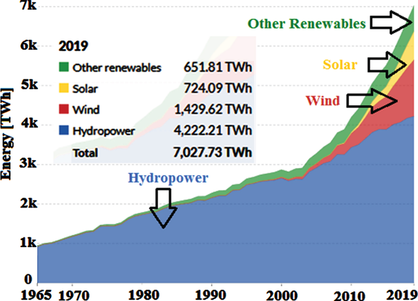
Renewable energy generation in world [2].

According to the Our World in Data [2] and MNRE (Ministry of New and Renewable Energy Resources), the current wind energy generation in India is 63.31 TWh (in 2019) and targeted the future goal of 175GW of renewable energy generation by 2022 [3], which is very large amount than the cited wind power potential of about 302GW in 2018 in a survey conducted by NIWE (National Institute of Wind Energy) [4].

The WS forecasting (WSF) and prediction (WSP) play an important role in power system planning and maintenance to meet the un-interrupted demand. Generally WSF and/or WSP are performed based on the time-scale, which is categorized into 4-types: 1) VST-WSF: very-short term, 2) ST-WSF: short-term, 3) MT-WSF: medium-term and 4) LT-WSF: Long-term [5–6]. The VST-WSF, ST-WSF, MT-WSF and LT-WSF are based on the time interval in order of “seconds to few minutes”, “(30 minutes to 24 hours)”, “(1 day to 1 week)”, and “(1 week to years)” respectively. Moreover, there are several methods and approaches of SWF/WSP are reported in the literature, which are mainly classified into: 1) Physical methods (PM), 2) Statistical methods (SM), 3) Artificial Intelligence based methods (AIM) and 4) Hybrid methods (HM).

According to the literature survey as mentioned in [7 –21], the wind energy (WE) generation is increasing resource in the world, which is the function of WS. The accurate WE/power prediction of wind farm output requires accurate prediction of WS. Therefore, prediction of WS is important for wind farms units’ maintenance, optimal power flow between conventional units and wind farms, electricity marketing bidding, power system generators scheduling, energy reserve, storages planning and scheduling. Hence, predictions of WS performed by various researchers are discussed in several published articles [5 –21].

The main contribution of this paper is to develop a novel NN approach based on a real-time logged historical dataset of 2015–2017 for STWF, which is further applicable to forecast the WS for those locations where no metrological station is available. The forecasted WS is used for wind resource assessment of wind turbines size matching to generate the optimal level of power potential.

The formulation of this manuscript is presented into six sub-sections, which includes the introduction in section-1 and study area and dataset collection for daily STWSF in section-2. The Section 3 represents the proposed framework, which includes the design of NNs and its performance measure indices are represented in section-4. Results demonstration and its discussion are represented in section-5 and finally conclusion is shown in section-6.

2 Study area and dataset collection

The Nainital (latitude [ºN] 29°23’31”N and longitude [ºE] 79°27’15”E and altitude [m] 1938 (6358 ft)) site in the Kumaon foothills of the outer Himalayas, is considered for the study in this chapter as shown in the Fig. 2. Nainital is covered by the Himalayas and it has huge potential of wind energy throughout the year. Here mean value of WS varies from o.768–1.294, 0.685–1.187 and 1.06–1.366 m/s for the year of 2015, 2016 and 2017 respectively throughout the year. Moreover, it is surrounded by Himalaya’s hills, so, the average air-temperature, average humidity, and average pressure are 16.44 °C (varies through the year: –0.8 to 34), 74.61% (varies through the year: 9 to 100) and 864.2 hPa (varies through the year: 851 to 874) for the year 2015. Similarly for year 2016, the average air-temperature, average humidity, and average pressure are 17.16 °C (varies through the year: –49.8 to 58.4), 71.34% (varies through the year: 5 to 100) and 863.14 hPa (varies through the year: 853 to 874). According to historical record, the maximum and minimum WS varies from 9.8 to 0 (m/s), 9.6 to 0 (m/s) and 10.9 to 0 (m/s) for the year of 2015, 2016, and 2017 respectively throughout the year as shown in Table 1 (for 2015) and Fig. 3 (for 2016).

Fig. 2

Location of Nainital city of Uttrakhand, India.

Table 1

Statistical analysis of recorded 2015 dataset’s variable of wind speed (ws) (in m/s)

Month	Min.	Mean	Max.	STD	Var.
Jan.	0	1.066	8.1	0.958	0.917
Feb.	0	1.294	8.8	1.189	1.413
March	0	1.29	7.6	1.113	1.238
April	0	1.105	9.1	0.97	0.942
May	0	1.241	9.8	1.052	1.107
June	0	0.994	6.6	0.873	0.762
July	0	0.792	4.7	0.709	0.503
Aug.	0	0.793	4.4	0.737	0.544
Sep.	0	0.786	4.8	0.829	0.688
Oct.	0	0.768	5.1	0.823	0.677
Nov.	0	0.85	5.9	0.858	0.736
Dec.	0	1.045	4.9	0.902	0.814
Average	0	1.002	6.65	0.918	0.862

Fig. 3

Statistical analysis of recorded 2016 dataset’s variable of wind speed (ws) (in m/s).

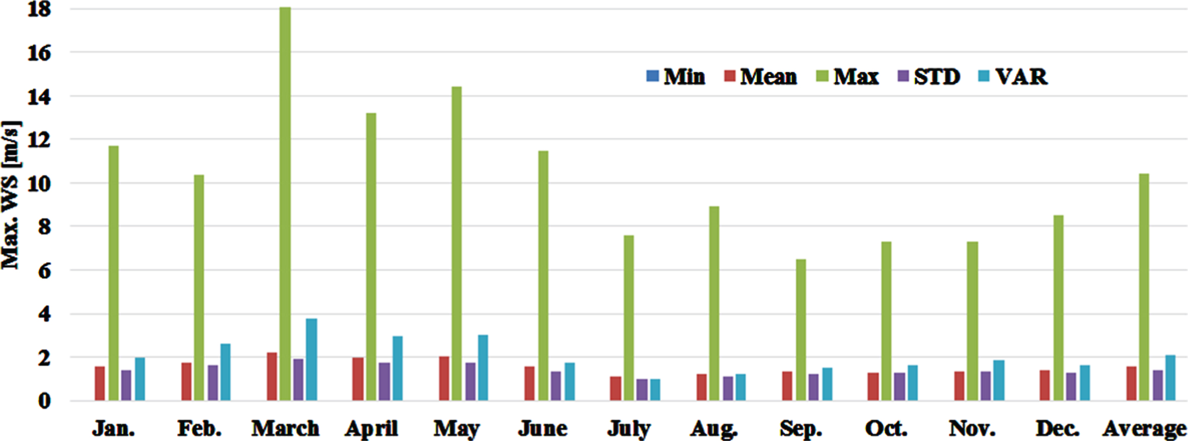
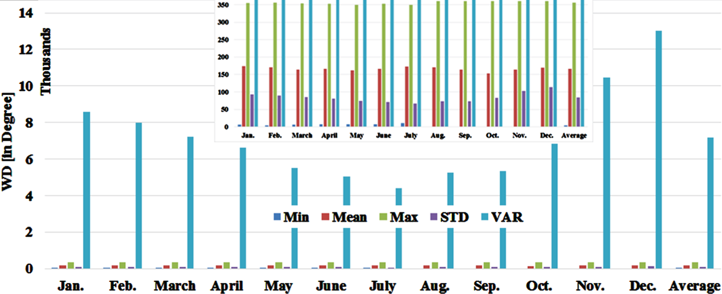
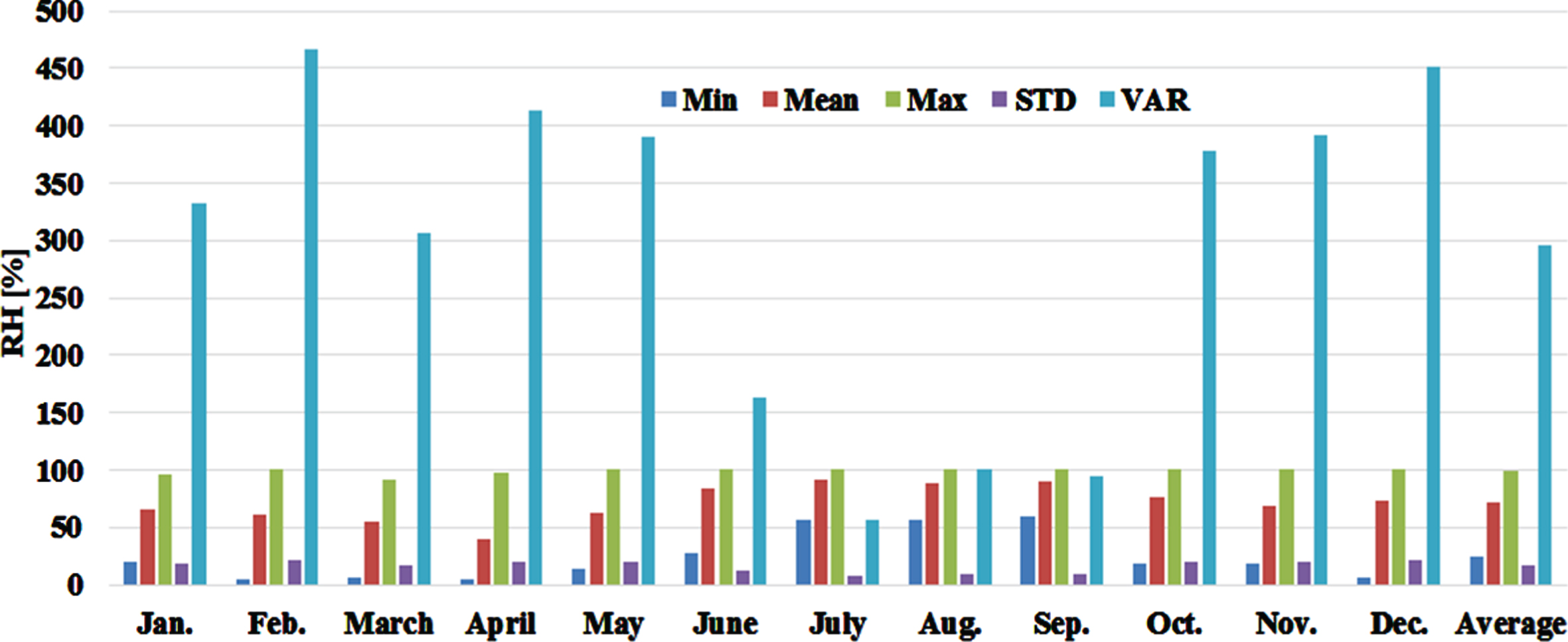
The historical data from meteorological data recording station, has been collected for the academic use. The several variables (i.e., WS: wind speed, WD: wind direction, Temp.: temperature, RH: relative humidity, P: pressure, Pre: precipitation) were collected at the one minute interval of the time. The recorded data from 1^st Jan 2015 to 31^st Dec. 2017 were used for the study. The further statistical analysis of the recorded data sets are represented in Tables 1 5 and Figs. 3 7, which are minimum value, maximum value, mean, standard deviation (STD) and variance (VAR) for the year of 2015 and 2016 respectively.

Table 2

Statistical analysis of recorded 2015 dataset’s variable of max. Horizontal wind speed (maxws) (in m/s)

Month	Min.	Mean	Max.	STD	Var.
Jan.	0	1.57	11.4	1.41	1.98
Feb.	0	1.909	15.5	1.72	2.95
March	0	1.914	10.6	1.62	2.64
April	0	1.758	17.8	1.51	2.27
May	0	2.034	18.4	1.71	2.92
June	0	1.614	11.4	1.4	1.97
July	0	1.288	8.1	1.11	1.23
Aug.	0	1.297	8.4	1.15	1.33
Sep.	0	1.312	7.4	1.3	1.69
Oct.	0	1.25	7.4	1.27	1.61
Nov.	0	1.304	7.3	1.28	1.63
Dec.	0	1.522	6.9	1.33	1.77
Average	0	1.564	10.88	1.4	2

Table 3

Statistical analysis of recorded 2015 dataset’s variable of wind direction (wd) (in degree)

Month	Min.	Mean	Max.	STD	Var.
Jan.	3	168.89	354	90.66	8220.12
Feb.	4	163.68	355	87.73	7696.23
March	5	161.56	355	83.44	6963.01
April	6	158.01	349	77.33	5979.96
May	7	159.41	349	76.45	5844.88
June	7	160.69	350	77.09	5942.22
July	8	167.78	347	71.48	5109.62
Aug.	8	168.42	353	66.82	4465.43
Sep.	5	158.8	351	64.79	4198.04
Oct.	5	155.03	354	75.02	5628.66
Nov.	3	164.53	354	87.64	7681.4
Dec.	5	174.07	354	92.92	8633.99
Average	5.5	163.41	352.08	79.28	6363.63

Table 4

Statistical analysis of recorded 2015 dataset’s variable of relative humidity (RH) (in %)

Month	Min.	Mean	Max.	STD	Var.
Jan.	15	73.5	100	20.52	421
Feb.	9	72.57	98	18.29	334.5
March	15	71.17	98	18	324
April	19	68.81	99	18.75	351.6
May	7	52.66	96	19.88	395.1
June	17	68.55	100	22.92	525.4
July	59	91.22	100	8.409	70.71
Aug.	57	91.25	100	8.346	69.66
Sep.	42	87.05	100	11.46	131.2
Oct.	17	75.05	99	18.55	344.2
Nov.	24	71	97	18.87	356
Dec.	9	72.47	97	19.43	377.5
Average	24.2	74.61	98.7	16.95	308.4

Table 5

Statistical analysis of recorded 2015 dataset’s variable of Air Temperature (°C)

Month	Min.	Mean	Max.	STD	Var.
Jan.	0	8.08	17.2	4.32	18.66
Feb.	1.4	11.05	22.7	4.515	20.39
March	2.9	13.88	26	4.882	23.83
April	7.6	17.29	28.3	4.6	21.16
May	10.9	22.62	32.6	5.045	25.45
June	14.9	22.89	34	3.808	14.5
July	17.4	21.95	28.6	2.051	4.208
Aug.	16.7	21.78	27.3	2.074	4.302
Sep.	11.6	20.38	27.4	3.535	12.49
Oct.	6.8	16.6	27.5	4.954	24.54
Nov.	6.2	13.37	23	4.921	24.21
Dec.	–0.8	7.473	25	5.363	28.76
Average	7.967	16.45	26.63	4.172	18.54

Fig. 4

Statistical analysis of recorded 2016 dataset’s variable of max. Horizontal wind speed (maxws) (in m/s).

Fig. 5

Statistical analysis of recorded 2016 dataset’s variable of wind direction (WD) (in degree).

Fig. 6

Statistical analysis of recorded 2016 dataset’s variable of relative humidity (RH) (in %).

Fig. 7

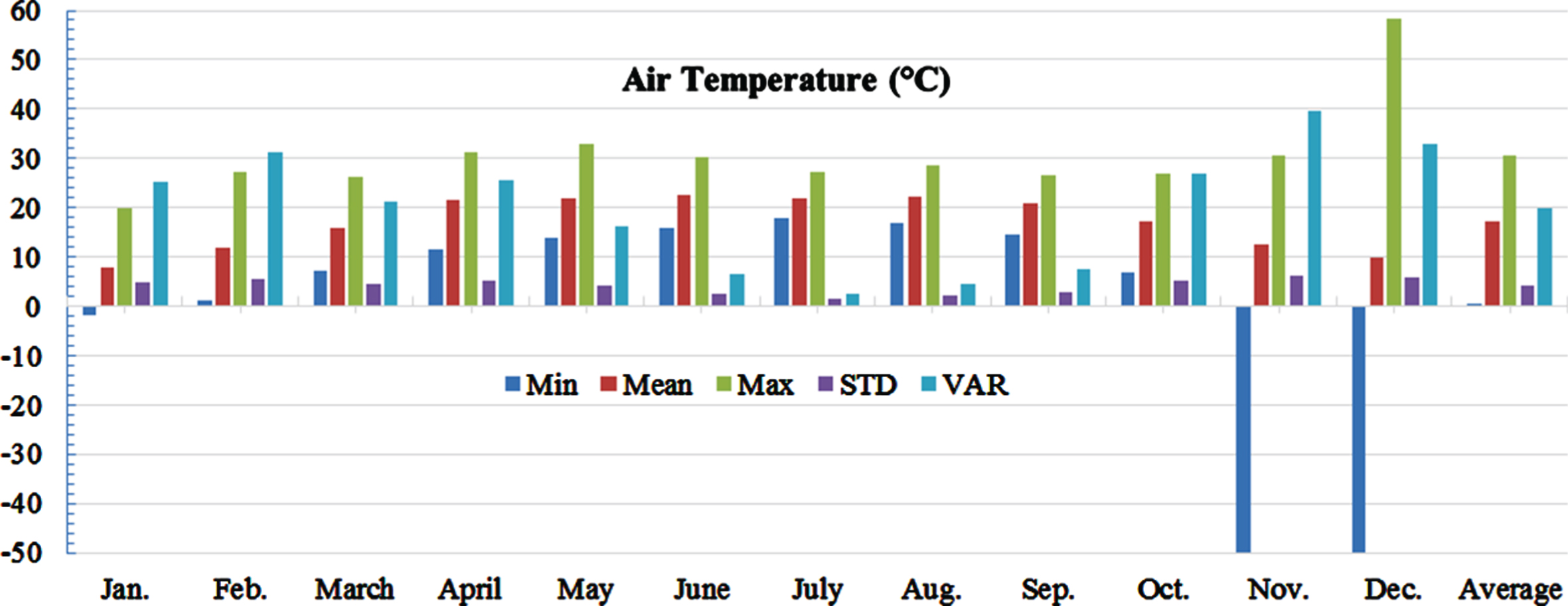
Statistical analysis of recorded 2016 dataset’s variable of Air Temperature (°C).

The historical data of WS is logged per minute basis, which is started at [00 : 01 : 00] to [23 : 59 : 00] for each day throughout the year. Due to some unwanted weather condition and/or instrumental/ operational/ technical and human errors, there are some missing values and/or spikes in the logged time series WS data Therefore, in this study, data pre-processing technique is employed to rectify the logged data by filling the appropriate missing values and removing the spikes (if any). The rectified data for the year 2015 is shown in Fig. 8 for better understanding. In Fig. 8(a) to Fig. 8(l), the historical and processed data are represented for each month starting from January to December, which is represented by dark black colour and gray colour for logged and processed (after filling missing value and/or spikes removal) data set respectively.

Fig. 8

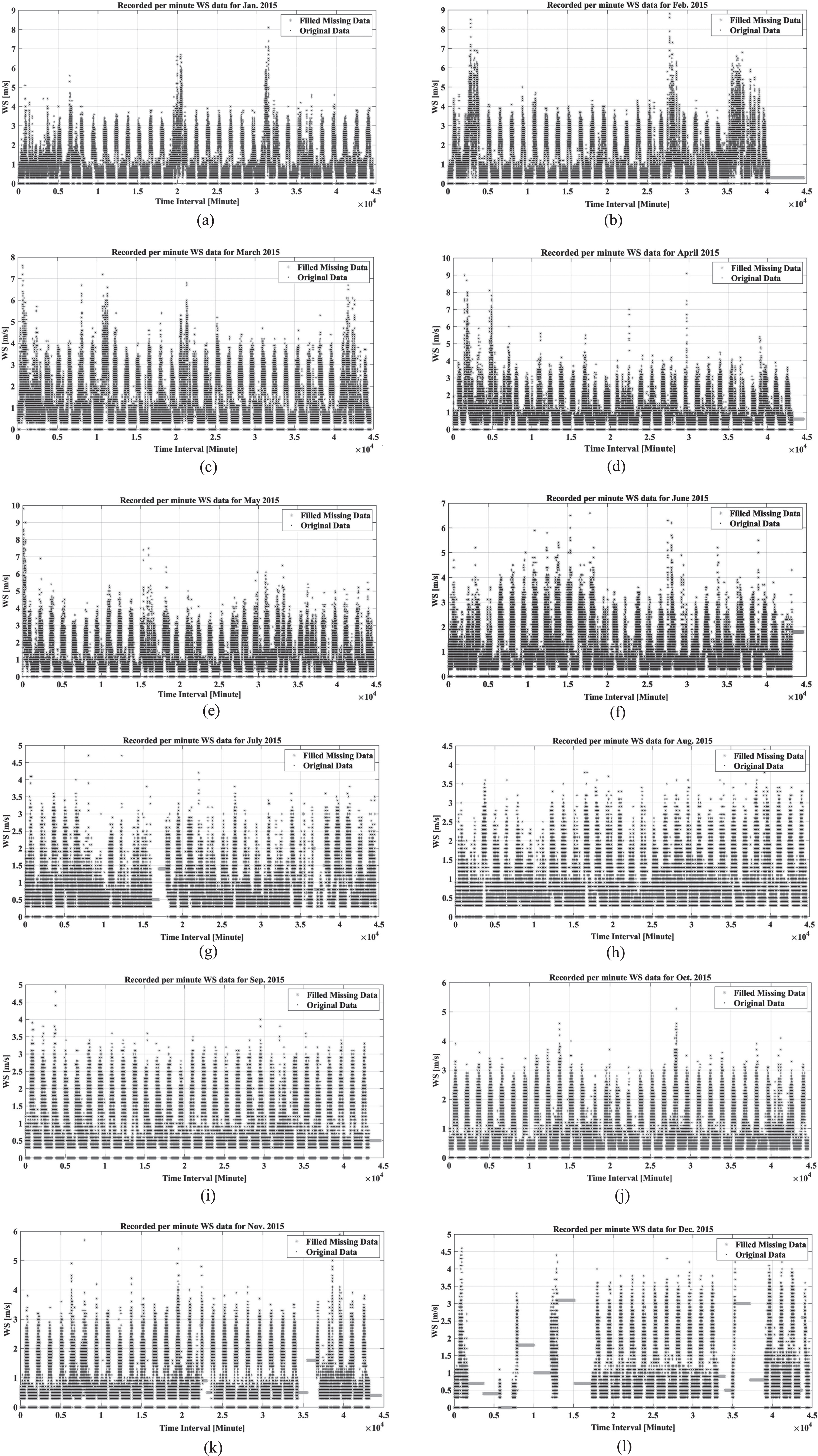
Per minute WS representation for original historical data and filled missing value data.

For the further analysis of WS using ANN, the per minute dataset is converted into the daily prediction, which is divided into two sub-data set (training data 70% and testing data 30%) and testing dataset is divided into multiple file for further use.

3 Proposed hybrid approach

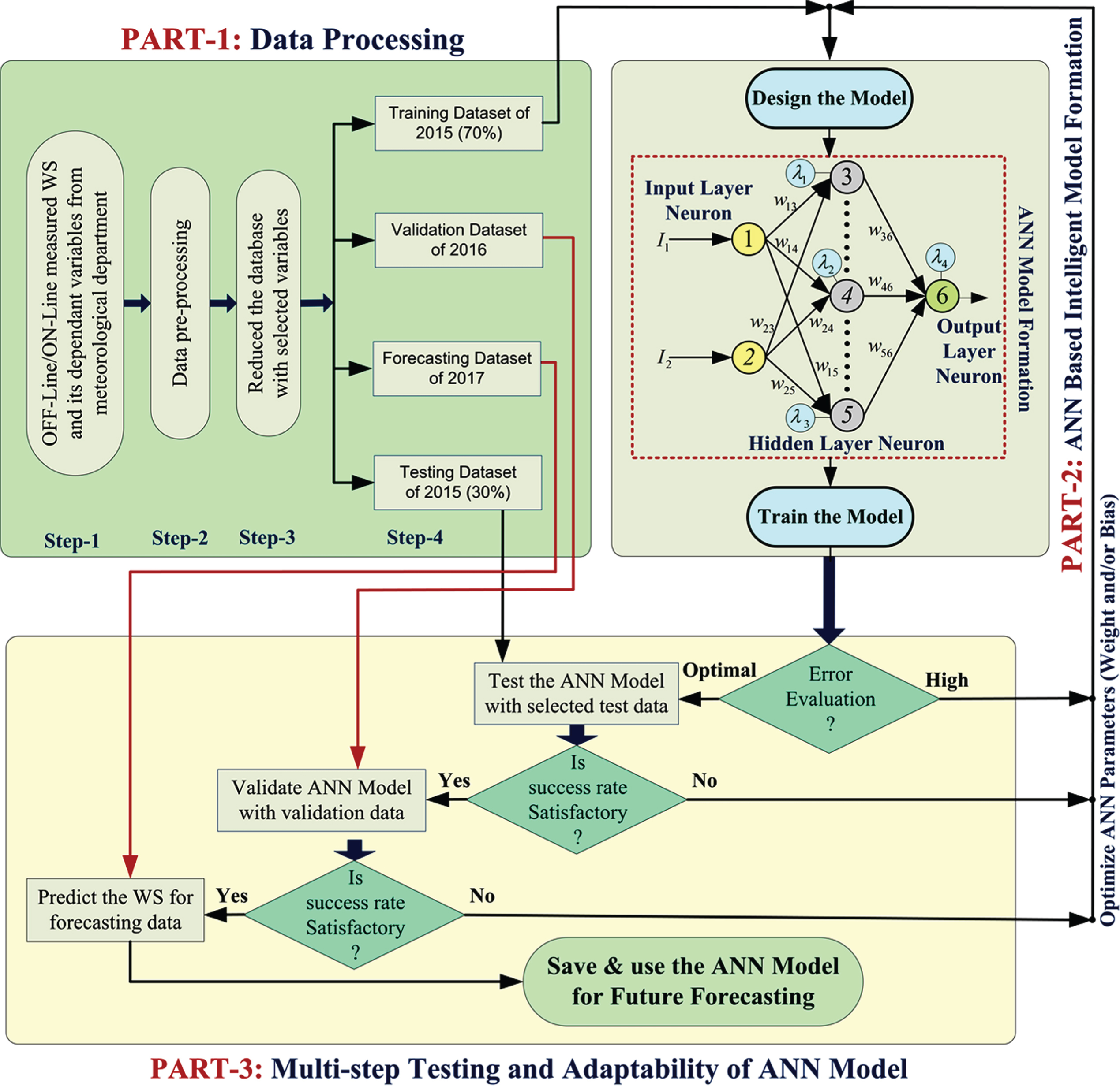
The developed approach, which is proposed in this study is formulated into three parts, is represented in Fig. 9. These three main parts such as: 1) Data processing part, 2) ANN model design and training part, and 3) Multi-step testing and adaptability verification of the approach. First two parts (PART-1 and PART-2) include the several steps, which are represented as follows: Part-1 includes four steps and Part-2 includes two steps. The dataset collection, data pre-processing, and four different data files (i.e., training, testing, validation, and forecasting) formation are included in the Part-1. In the first step, a recorded meteorological logged dataset from the sites has been collected with different variables. The developed all four data files are not similar to each other. The training data file is used for ANN models design and developed ANN models learns the WS forecasting property based on evaluated per day dataset of Nainital city. After training phase, testing phase is performed to test the trained model performance. If testing phase performance is acceptable then validation data file is used to test the model again. Therefore, trained model is tested multiple time to cross check the model performance by using different datasets (i.e., testing, validation and forecasting dataset).

Fig. 9

Proposed approach for WSFP.

3.1 Neural network (NN) overview

The BP (back propagation) algorithm based MLP (multilayer perceptron) type of NN’s architecture is used in this study as represented in Fig. 10 [22 –26]. The I₁ and I₂ are the assumed input variables which are connected to input neuron of 1 and 2 respectively. Neuron number 1 and 2 are further connected with hidden layer neurons of 2,4,5 through the weight vector of w^ih (w₁₃, w₁₄, w₁₅, w₂₃, w₂₄, and w₂₅). The output of the neuron 3,4,5 are connected to the output neuron number 6 though the weight vector of w^ho (w₃₆, w₄₆, and w₅₆) as shown in the Fig. 10. The mathematical model for developed NN is mentioned in Eq. 1 to 7 which includes weight value w^ih and w^ho.

Fig. 10

Developed NN Model Architecture [10 , 22–26].

At input Layer: the computation at the ith neuron: $Data sample selection = G (y_{i}) = y_{i}, i = 1, 2, . . . ., n$ (1) $G (y_{0}) = 1$ (2)

At hidden Layer: The computation at the hth neuron is: $\begin{matrix} Input value net (Hi) = \\ U_{h} = \sum_{i = 0}^{n} w_{ih}^{I} G (y_{i}), h = 1, 2, . . . ., p \end{matrix}$ (3) $\begin{matrix} output value of (Hi) \\ out (Hi) = G (U_{h}) = \frac{1}{1 + e^{- U_{h}}} h = 1, 2, . . . ., p \\ , \end{matrix}$ (4) $G (U_{0}) = 1 .$ (5)

At output Layer: The computation at the jth neuron is: $\begin{matrix} Input value of (Oi) \\ out (Oi) = f_{j} = \sum_{h = 0}^{p} w_{hj}^{H} G (U_{h}), j = 1, 2, . . . ., p \end{matrix}$ (6) $\begin{matrix} output value (Oi) \\ out (Oi) = G (f_{j}) = \frac{1}{1 + e^{- f_{j}}} j = 1, 2, . . . ., p \end{matrix}$ (7) where, G (·) = activation function.

4 Model performance evaluation metrics

The model performance computation is the procedure to calculate the characteristics in form of its performance, which shows the model’s capability to WS forecasting which are MAE (Mean Absolute Error), MAPE (Mean Absolute Percentage Error) and RMSE (Root Mean Square Error) used in this study. These performance indices are calculated for the NN models as given below: $MAE = \frac{1}{N} \sum_{t = 1}^{K} | \hat{f} (t) - f_{h} (t) |$ (8) $MAPE = (\frac{1}{N} \sum_{t = 1}^{K} | \frac{\hat{f} (t) - f_{h} (t)}{f_{h} (t)} |) \times 100$ (9) $RMSE = \sqrt{\frac{1}{N} \sum_{t = 1}^{K} {(\hat{f} (t) - f_{h} (t))}^{2}}$ (10)

Where, $\hat{f} (t)$ and f_h (t) are the forecasted and historical solar radiation at time interval k respectively, K is the total number of forecasted and historical data samples.

5 Demonstration of results

The experimental results demo for daily WS forecasting is signified into two categories: 1) One-Step Ahead (OSA) forecasting and 2) Multi-Step Ahead (MSA) forecasting. The MSA forecasting is performed upto two more step-ahead based forecasting (TSA: two-step ahead and ThSA: three-step ahead). The information of the used dataset is tabulated in Table 6 and obtained best optimal results from each case study have been demonstrated in Table 8. Table 7 tabulates the total number of developed NN models in this study.

Table 6
Dataset used for NNs model formation for ELF

Years Per-minute recorded data Converted data into Hourly then daily

2015 Data sample 01-01-2015 00 : 01 : 00 to 31-12-2015 23 : 59 : 00 8760–365

2016 Data sample 01-01-2015 00 : 01 : 00 to 31-12-2015 23 : 59 : 00 8760–365

2017 Data sample 01-01-2015 00 : 01 : 00 to 31-12-2015 23 : 59 : 00 8760–365

Years	Per-minute recorded data	Converted data into Hourly then daily
2015 Data sample	01-01-2015 00 : 01 : 00 to 31-12-2015 23 : 59 : 00	8760–365
2016 Data sample	01-01-2015 00 : 01 : 00 to 31-12-2015 23 : 59 : 00	8760–365
2017 Data sample	01-01-2015 00 : 01 : 00 to 31-12-2015 23 : 59 : 00	8760–365

Table 7

Developed NNs models for multi-step forecasting

Used dataset type for NN model	OSA	TSA	ThSA
Training Dataset of 2015 ( 70%)	1	1	1

Table 8

NNs performance for ELF: MAPE value

Performance phase	Daily forecasting
	OSA	TSA	ThSA
2015 Data (Testing phase)	5.845	5.859	6.014
2016 Data (Testing phase#1)	5.148	5.439	5.655
2017 Data (Testing phase#2)	6.035	6.227	6.407

These three case studies (i.e., OSA, TSA, and ThSA forecasting) are developed and analyzed with consideration of it distinct and valuable application in the power system such as power system planning, power system maintenance, power system scheduling, power system unit commandment, economic load dispatch management, OPF (optimal power flow) analysis, automatic generation control etc.

5.1 One-step ahead forecasting

Here, one day-ahead forecasting demonstration of the results for testing phase are represented tabulated in Table 9 and its detailed representation is represented in Fig 11 and Fig. 12 for the tested dataset of year 2016 and 2017 respectively. From the test result analysis, it is shown that the average value of MAPE for Monday to Sunday are 3.23, 4.99, 5.15, 6.57, 4.23, 5.92, and 4.69 respectively for the January of year of 2016. And for the January of year 2017, the testing results are 9.47, 3.98, 9.59, 8.21, 9.85, 3.09, and 10.5 for the day of Monday to Sunday respectively. In the both cases (2016 and 2017), the weekly average value of MAPE are 4.966 and 7.813 respectively in January, which are highly acceptable for the forecasting problems. For the detail analysis of each day of each month is demonstrated in the Tables 10 and 11 for the year of 2016 and 2017 dataset.

Table 9
Daily WS forecasting error for Nainital

Used dataset Phase of operation MAE RMSE MAPE

2015 Dataset Training phase 0.139 0.275 2.14

Testing Phase 0.471 0.702 5.845

2016 Dataset Testing Phase 0.582 2.39 5.148

2017 Dataset Testing Phase 0.563 1.835 6.035

Used dataset	Phase of operation	MAE	RMSE	MAPE
2015 Dataset	Training phase	0.139	0.275	2.14
	Testing Phase	0.471	0.702	5.845
2016 Dataset	Testing Phase	0.582	2.39	5.148
2017 Dataset	Testing Phase	0.563	1.835	6.035

Fig. 11

MAPE analysis for OSA daily WS forecasting (Test#1 : 2016 dataset).

Fig. 12

MAPE analysis for OSA daily WS forecasting (Test#2 : 2017 dataset).

Table 10

The OSA MAPE for Daily WS Forecasting (Test#1 : 2016 Dataset)

	Monday	Tuesday	Wednesday	Thursday	Friday	Saturday	Sunday	Weekly average
January	3.23	4.99	5.14	6.57	4.23	5.92	4.69	4.97
February	3.9	3.49	4.53	7.1	4.88	5.31	8.23	5.35
March	3.59	1.65	4.4	7.53	3.8	2.98	5.76	4.24
April	4.59	5.12	2.85	5.87	4.1	5.31	3.95	4.54
May	7.5	4.07	5.54	4.76	8.1	5.98	8.49	6.35
June	1.37	3.44	4.77	5.89	3.11	4.88	6.73	4.31
July	2.33	6.64	3.32	4.29	7.01	5.91	2.84	4.62
August	3.42	6.8	4.98	4.49	8.75	4.02	7.11	5.65
September	4.2	6.29	4.32	4.94	8.07	4.94	2.62	5.05
October	6.82	2.55	3.83	4.17	8.63	4.53	1.62	4.59
November	8.43	6.44	7.25	6.49	8.74	6.54	8.67	7.51
December	2.23	4.64	6.28	5.63	3.32	3.76	6.28	4.59
Monthly average	4.3	4.68	4.77	5.64	6.06	5.01	5.58	5.15

Table 11

The OSA MAPE for Daily WS Forecasting (Test#2 : 2017 Dataset)

	Monday	Tuesday	Wednesday	Thursday	Friday	Saturday	Sunday	Weekly average
average
January	9.47	3.98	9.59	8.21	9.85	3.09	10.5	7.81
February	5.7	4.68	5.89	5.17	4.31	7.12	5.74	5.52
March	4.29	3.74	7.21	5.03	5.73	4.76	5.2	5.14
April	3.06	4.83	9.99	6.23	7.63	2.86	8.31	6.13
May	1.45	4.68	7.22	4.27	2.63	3.43	5.4	4.15
June	4.02	5.68	7.5	7.45	4.74	7.36	9.22	6.57
July	2.2	4.87	5.43	6.41	6.73	4.66	6.86	5.31
August	5	6.14	6.31	9.86	9.64	4.86	1.85	6.24
September	6.81	8.17	7.13	8.64	7.73	8.77	4.98	7.46
October	5.66	4.8	6.83	4.87	3.99	6	3.4	5.08
November	4.21	7.33	9.65	6.13	6.74	4.89	6.18	6.45
December	3.05	8.68	8.37	7.85	5.52	8.86	3.74	6.58
Monthly average	4.58	5.63	7.59	6.68	6.27	5.55	5.95	6.04

5.2 Multi-step ahead forecasting

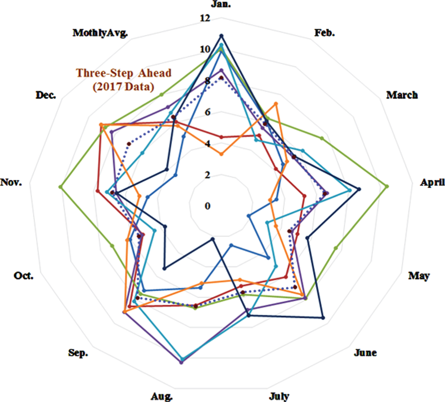
In this section, the results demonstration of daily-ahead WS forecasting for TSA ahead and ThSA forecasting, which are represented in Figs. 13 16. The Figs. 13 and 14 show the TSA performance demonstration for testing dataset of year 2016 and 2017 respectively. Whereas, Figs. 15 and 16 represent the ThSA performance demonstration for testing dataset of year 2016 and 2017 respectively. The detailed analysis of the performance for each model is tabulated in the Tables 12 13 (for TSA) and Tables 14 15 (for ThSA). Tables 12 and 14 represents the testing phase results for the logged dataset of the year 2016 for TSA and ThSA forecasting respectively. Similarly, Tables 13 and 15 represents the testing phase results for the logged dataset of the year 2017 for TSA and ThSA forecasting respectively.

Fig. 13

MAPE analysis for TSA daily WS forecasting (Test#1 : 2016 dataset).

Fig. 14

MAPE analysis for TSA daily WS forecasting (Test#2 : 2017 dataset).

Fig. 15

MAPE analysis for ThSA daily WS forecasting (Test#1 : 2016 dataset).

Fig. 16

MAPE analysis for ThSA daily WS forecasting (Test#2 : 2017 dataset).

Table 12

The TSA MAPE for Daily WS Forecasting (Test#1 : 2016 Dataset)

	Monday	Tuesday	Wednesday	Thursday	Friday	Saturday	Sunday	Weekly average
average
January	3.45	9.21	5.36	6.8	4.46	6.15	4.88	5.76
February	4.12	3.71	4.75	9.33	5.11	5.54	8.42	5.85
March	3.81	1.87	4.62	7.76	4.03	3.21	5.95	4.46
April	4.81	5.34	3.07	6.1	4.33	5.54	4.14	4.76
May	7.72	4.29	5.76	4.99	8.33	6.21	8.68	6.57
June	1.59	3.66	4.99	6.12	3.34	5.11	6.92	4.53
July	2.55	6.86	3.54	4.52	7.24	6.14	3.03	4.84
August	3.64	7.02	5.2	4.72	8.98	4.25	7.3	5.87
September	4.42	6.51	4.54	5.17	8.3	5.17	2.81	5.27
October	7.04	2.77	4.05	4.4	8.86	4.76	1.81	4.81
November	8.65	6.66	7.47	6.72	8.97	6.77	8.86	7.73
December	2.45	4.86	6.5	5.86	3.55	3.99	6.47	4.81
Monthly average	4.52	5.23	4.99	6.04	6.29	5.24	5.77	5.44

Table 13

The TSA MAPE for Daily WS Forecasting (Test#2 : 2017 Dataset)

	Monday	Tuesday	Wednesday	Thursday	Friday	Saturday	Sunday	Weekly average
average
January	9.69	4.2	9.81	8.44	10.1	3.12	10.7	8.01
February	5.92	4.9	6.11	5.4	4.54	7.16	5.93	5.71
March	4.51	3.96	7.43	5.26	5.96	4.79	5.39	5.33
April	3.28	5.05	10.2	6.46	7.86	2.89	8.5	6.32
May	1.67	4.9	7.44	4.5	2.86	3.47	5.59	4.35
June	4.24	5.9	7.72	7.68	4.97	7.4	9.41	6.76
July	2.42	5.09	5.65	6.64	6.96	4.69	7.05	5.5
August	5.22	6.36	6.53	10.1	9.87	4.89	2.04	6.43
September	7.03	8.39	7.35	8.87	7.96	8.8	5.17	7.65
October	5.88	5.02	7.05	5.1	4.22	6.03	3.59	5.27
November	4.43	7.55	9.87	6.36	6.97	4.92	6.37	6.64
December	3.27	8.9	8.59	8.08	5.75	8.89	3.93	6.77
Monthly average	4.8	5.85	7.81	6.91	6.5	5.59	6.14	6.23

In the TSA daily-WS forecasting case study, the average maximum and minimum MAPE for testing phase is 4.46–7.727 (for 2016 test dataset) and 4.34–8.01 (for 2017 test dataset), and the overall-average MAPE for all days of the months is 5.44 (for 2016 test dataset) and 6.23 (for 2017 test dataset).

Similarly, in the ThSA daily-WS forecasting case study, the average maximum and minimum MAPE for testing phase is 4.64–7.91 (for 2016 test dataset) and 4.53–8.19 (for 2017 test dataset), and the overall-average MAPE for all days of the months is 5.66 (for 2016 test dataset) and 6.41 (for 2017 test dataset).

Therefore, after analyzing Tables 12 to Table 15, it is summarized that designed NN models for TSA and ThSA forecasting for daily WS forecast are more acceptable and it can be implemented for future applications.

Table 14

The ThSA MAPE for Daily WS Forecasting (Test#1 : 2016 Dataset)

	Monday	Tuesday	Wednesday	Thursday	Friday	Saturday	Sunday	Weekly average
average
January	3.63	9.39	5.54	6.99	4.65	6.34	5.03	5.94
February	4.3	3.89	4.93	12.5	5.3	5.73	8.57	6.46
March	3.99	2.05	4.8	7.95	4.22	3.4	6.1	4.64
April	4.99	5.52	3.25	6.29	4.52	5.73	4.29	4.94
May	7.9	4.47	5.94	5.18	8.52	6.4	8.83	6.75
June	1.77	3.84	5.17	6.31	3.53	5.3	7.07	4.71
July	2.73	7.04	3.72	4.71	7.43	6.33	3.18	5.02
August	3.82	7.2	5.38	4.91	9.17	4.44	7.45	6.05
September	4.6	6.69	4.72	5.36	8.49	5.36	2.96	5.45
October	7.22	2.95	4.23	4.59	9.05	4.95	1.96	4.99
November	8.83	6.84	7.65	6.91	9.16	6.96	9.01	7.91
December	2.63	5.04	6.68	6.05	3.74	4.18	6.62	4.99
Monthly average	4.7	5.41	5.17	6.48	6.48	5.43	5.92	5.66

Table 15

The ThSA MAPE for Daily WS Forecasting (Test#2 : 2017 Dataset)

	Monday	Tuesday	Wednesday	Thursday	Friday	Saturday	Sunday	Weekly average
average
January	9.87	4.38	9.99	8.63	10.3	3.31	10.8	8.19
February	6.1	5.08	6.29	5.59	4.73	7.35	6.08	5.89
March	4.69	4.14	7.61	5.45	6.15	4.98	5.54	5.51
April	3.46	5.23	10.4	6.65	8.05	3.08	8.65	6.5
May	1.85	5.08	7.62	4.69	3.05	3.66	5.74	4.53
June	4.42	6.08	7.9	7.87	5.16	7.59	9.56	6.94
July	2.6	5.27	5.83	6.83	7.15	4.88	7.2	5.68
August	5.4	6.54	6.71	10.3	10.1	5.08	2.19	6.61
September	7.21	8.57	7.53	9.06	8.15	8.99	5.32	7.83
October	6.06	5.2	7.23	5.29	4.41	6.22	3.74	5.45
November	4.61	7.73	10.1	6.55	7.16	5.11	6.52	6.82
December	3.45	9.08	8.77	8.27	5.94	9.08	4.08	6.95
Monthly average	4.98	6.03	7.99	7.1	6.69	5.78	6.29	6.41

6 Conclusions

In this study, a multi-step-ahead time-series wind speed forecasting model for smart-grid application has been proposed and its performance has been demonstrated, and validated by using real-time logged dataset of the year 2015 to 2017, which has been collected from an Indian city of Nainital. The multi-step ahead forecasting has been executed recursively using different NNs for daily wind speed forecasting based on OSA (1 day), TSA (2 days), and ThSA (3 days) forecasting, and this procedure is repeated until a time step of 3 days. The proposed models are competent to solve the linear and/or non-linear problems such as STWSF, which is a highly non-linear problem, which has been handled by proposed method in an efficient way with less computational burden.

Footnotes

Acknowledgments

“The authors extend their appreciation to the Researchers Supporting Project at King Saud University, Riyadh, Saudi Arabia, for funding this research work through the project number RSP-2020/278”.

References

Chapter 1 in Renewable energy devices and systems with simulations in MATLAB and ANSYS, Editor: F. Blaabjerg and D.M. Lonel, CRC Press LLC.

Hannah Ritchie and Max Roser, “Renewable Energy”, https://ourworldindata.org/renewable-energy (Accessed on-22-07-2020).

Ministry of New and Renewable Energy Resources (MNRE), https://mnre.gov.in/filemanager/annual-report/2016-2017/EN/pdf/1.pdf.

Ministry of New and Renewable Energy Resources (MNRE), https://mnre.gov.in/file-manager/akshay-urja/october-2017/Images/20-25.pdf. (Accessed on-22-02-2019).

Alencar

D.B.

, et al. HybridApproachCombining SARIMA and Neural Networks for Multi-Step Ahead Wind Speed Forecasting in Brazil, IEEE Access 6 (2018), 55986–55994. 10.1109/ACCESS.2018.2872720.

Sheela

K.G.

, Neural network based hybrid computing model for wind speed prediction, Neurocomputing. doi: https://dx-doi-org.web.bisu.edu.cn/10.1016/j.neucom.2013.06.008.

Wang

, et al. Short-term wind speed prediction using an extreme learning machine model with error correction, Energy Conversion and Management 162 (2018), 239–250. doi: https://doi.org/10.1016/j.enconman.2018.02.015.

, et al. A new hybrid model optimized by an intelligent optimization algorithm for wind speed forecasting, Energy Conversion and Management 85 (2014), 443–452. Doi: https://dx-doi-org.web.bisu.edu.cn/10.1016/j.enconman.2014.05.058.

Shi

, et al. Evaluation of hybrid forecasting approaches for wind speed and power generation time series, Renewable and Sustainable Energy Reviews 16 (2012), 3471–3480. Doi: 10.1016/j.rser.2012.02.044.

10.

Cadenas

and Rivera

, Wind speed forecasting in three different regions of Mexico, using a hybrid ARIMA-ANN model, Renewable Energy 35 (2010), 2732–2738. Doi: https://doi.org/10.1016/j.renene.2010.04.022.

11.

Wang

, et al. Analysis and application of forecasting models in wind power integration: A review of multi-step-ahead wind speed forecasting models, Renewable and Sustainable Energy Reviews 60 (2016), 960–981. Doi: https://doi.org/10.1016/j.rser.2016.01.114.

12.

Azeem

, et al. k-NN and ANN Based Deterministic and Probabilistic Wind Speed Forecasting Intelligent Approach, Journal of Intelligent & Fuzzy Systems 35(5) (2018), 5021–5031. Doi: 10.3233/JIFS-169786

13.

Malik

and Yadav

A.K.

, A novel hybrid approach based on relief algorithm and fuzzy reinforcement learning approach for predicting wind speed, Sustainable Energy Technologies and Assessments 43 (2020). Doi: https://doi.org/10.1016/j.seta.2020.100920

14.

Kumar

and Malik

, Generalized Regression Neural Network Based Wind Speed Prediction Model For Western Region Of India, in, Procedia Computer Science 93 (2016), 26–32. Doi: 10.1016/j.procs.2016.07.177.

15.

Garg

, et al. Infogain Attribute Evaluator and ANN Based Wind Speed Prediction Model for Rajasthan, North-West Region of India, in, Proc. of the Intl. Conf. on Nanotechnology for Better Living 3(1) (2016), 233. Doi: 10.3850/978-981-09-7519-7nbl16-rps-233.

16.

Savita1 , et al., Wind Speed and Power Prediction of Prominent Wind Power Potential States in India using GRNN, in Proc. IEEE ICPEICES-2016, pp. 1–6, 2016. Doi: 10.1109/ICPEICES.2016.7853220.

17.

Malik Savita

, Application of Artificial Neural Network for Long Term Wind Speed Prediction, in Proc. IEEE CASP-2016, pp. 217–222, 9–11 June 2016. Doi: 10.1109/CASP.2016.7746168.

18.

Azeem

, et al. Application of Waikato Environment for Knowledge Analysis Based Artificial Neural Network Models for Wind Speed Forecasting, in Proc. IEEE PIICON-2016, pp. 1–6, 25–27 Nov. 2016. Doi: 10.1109/POWERI.2016.8077352.

19.

Yadav

A.K.

and Malik

, 10-Min Ahead Forecasting of Wind Speed for Power Generation Using Nonlinear Autoregressive Neural Network, Book chapter in Applications of Artificial Intelligence Techniques in Engineering, Advances in Intelligent Systems and Computing 698 (2018), 235–244. Doi: https://doi.org/10.1007/978-981-13-1819-1_23.

20.

Vinoop

, et al. PSO-NN-Based Hybrid Model for Long-Term Wind Speed Prediction: A Study on 67 Cities of India, Book chapter in Applications of Artificial Intelligence Techniques in Engineering, Advances in Intelligent Systems and Computing 697 (2018), 319–327. Doi: https://doi.org/10.1007/978-981-13-1822-1_29.

21.

Yadav

A.K.

and Malik

, Short Term Wind Speed Forecasting For Power Generation In Hamirpur, Himachal Pradesh, India, Using Artificial Neural Networks, Book chapter in Applications of Artificial Intelligence Techniques in Engineering, Advances in Intelligent Systems and Computing 697 (2018), 263–271. Doi: https://doi.org/10.1007/978-981-13-1822-1_24.

22.

Yadav

A.K.

, et al. Selection of Most Relevant Input Parameters Using WEKA for Artificial Neural Network Based Solar Radiation Prediction Models, Renewable and Sustainable Energy Reviews 31 (2014), 509–519. Doi: https://doi.org/10.1016/j.rser.2013.12.008

23.

Malik

and Mishra

, Artificial Neural Network and Empirical Mode Decomposition Based Imbalance Fault Diagnosis of Wind Turbine Using TurbSim, FAST and Simulink, IET Renewable Power Generation 11(6) (2017), 889–902. Doi: 10.1049/iet-rpg.2015.0382

24.

Yadav

A.K.

, et al. Daily Array Yield Prediction of Grid-Interactive Photovoltaic Plant Using Relief Attribute Evaluator Based Radial Basis Function Neural Network, Renewable and Sustainable Energy Reviews 81(Part 2) (2018), 2115–2127. Doi: https://doi.org/10.1016/j.rser.2017.06.023.

25.

Malik

and Sharma

, EMD and ANN based Intelligent Fault Diagnosis Model for Transmission Line, Journal of Intelligent & Fuzzy Systems 32(4) (2017), 3043–3050. Doi: 10.3233/JIFS-169247.

26.

Arora

, et al. Wind Energy Forecasting Model for Northern-Western Region of India Using Decision Tree and MLP Neural Network Approach, Interdisciplinary Environmental Review 19(1) (2018), 13–30. Doi: https://doi.org/10.1504/IER.2018.089766.

Multi-step ahead time-series wind speed forecasting for smart-grid application

Abstract

Keywords

1 Introduction

Table 9 Daily WS forecasting error for Nainital Used dataset Phase of operation MAE RMSE MAPE 2015 Dataset Training phase 0.139 0.275 2.14 Testing Phase 0.471 0.702 5.845 2016 Dataset Testing Phase 0.582 2.39 5.148 2017 Dataset Testing Phase 0.563 1.835 6.035

Footnotes

Acknowledgments

References

Table 9
Daily WS forecasting error for Nainital

Used dataset Phase of operation MAE RMSE MAPE

2015 Dataset Training phase 0.139 0.275 2.14

Testing Phase 0.471 0.702 5.845

2016 Dataset Testing Phase 0.582 2.39 5.148

2017 Dataset Testing Phase 0.563 1.835 6.035