Optimizations for filter-based join algorithms in MapReduce

Abstract

Large-scale datasets collected from heterogeneous sources often require a join operation to extract valuable information. MapReduce is an efficient programming model for processing large-scale data. However, it has some limitations in processing heterogeneous datasets. This is because of the large amount of redundant intermediate records that are transferred through the network. Several filtering techniques have been developed to improve the join performance, but they require multiple MapReduce jobs to process the input datasets. To address this issue, the adaptive filter-based join algorithms are presented in this paper. Specifically, three join algorithms are introduced to perform the processes of filters creation and redundant records elimination within a single MapReduce job. A cost analysis of the introduced join algorithms shows that the I/O cost is reduced compared to the state-of-the-art filter-based join algorithms. The performance of the join algorithms was evaluated in terms of the total execution time and the total amount of I/O data transferred. The experimental results show that the adaptive Bloom join, semi-adaptive intersection Bloom join, and adaptive intersection Bloom join decrease the total execution time by 30%, 25%, and 35%, respectively; and reduce the total amount of I/O data transferred by 18%, 25%, and 50%, respectively.

Keywords

Join algorithms big data management query optimization MapReduce

1 Introduction

The advancement of many technological trends, such as smart devices, the Internet of Things, cloud computing services, web-based services, and social networks, have contributed to the massive amount of data being generated every day at unprecedented rate. Such technologies have led to the emergence of the era of Big Data, the era of processing Gigabytes, Terabytes, or even Petabytes of data. Consequently, Big Data analytics has become one of the hottest topics in the field of computer science. In this newly challenging world, data is everywhere, and the driving forces are access to ever-increasing volumes of data and our ever-increasing technological capabilities to mine that data for commercial insights [1]. According to the International Data Corporation report [2], the volume of data we created in 2017 reached about 19 Zettabytes (ZB=10²¹) and it is expected in 2025 that the volume of data we create and copy will reach 163 ZB.

Prior to the revolution of Big Data, companies were using traditional database management systems to store and analyze their data. However, the performance of such systems degrades significantly in the context of Big Data. This is due to the very characteristics of Big Data and the lack of scalability and flexibility of these systems. Various frameworks have been developed by industry and academia to overcome the limitations of the traditional database management systems for processing large-scale data. Among these are Google MapReduce [3], Yahoo PNUTS [4], Microsoft SCOPE [5], and Apache Spark [6]. These platforms combine an infrastructure of commodity machines that can scale up to millions of servers and can store databases up to Exabytes (EB=10¹⁸) of volume. Moreover, with their powerful failure handling mechanism, a large amount of data can be processed in a reasonable time in order to extract valuable information.

The analysis of large-scale data is attracting substantial interest from the communities of business and academia. It has the potential to enhance the decision-making process through identifying valuable hidden information in the data [7]. In most circumstances, a join operation is crucial to analyze heterogeneous datasets. To process huge amounts of raw data, an efficient, reliable, and scalable framework is required, one of which is MapReduce [3]. However, despite MapReduce’s merits, it has some limitations in performing the join operation. This is because MapReduce was originally designed to process homogeneous data rather than heterogeneous data [8]. The main problem of join processing in MapReduce is the large number of redundant records that are transferred through the network. Several techniques have been developed to alleviate this issue, such as the Filter-Based Joins [9 –15]. However, these techniques require additional MapReduce jobs to perform the join operation.

In this paper, we present optimizations for the state-of-the-art filter-based joins in order to perform the join operation within a single MapReduce job. The fundamental idea is to perform the processes of filters creation and redundant records elimination with the lowest cost possible in terms of I/O and total execution time. To achieve this, we introduce two strategies to dynamically compute and distribute the filters. Moreover, we provide analytical and experimental comparisons of the introduced join algorithms and the state-of-the-art filter-based joins.

The rest of the paper is organized as follows. Section 2 summarizes the related work, addresses their limitations, and positions our paper with respect to existing literature. Section 3 introduces the implementation of the adaptive filter-based join algorithms. Section 4 provides a cost-based comparison of the filter-based joins. Section 5 presents the experimental results. Finally, Section 6 concludes the paper and discusses future work.

2 Related work

There has been extensive research in recent years to optimize join processing in the MapReduce framework [10 , 16–21]. Al-Badarneh and Rababa [22] classified join algorithms in MapReduce into four categories: standard joins, filter-based joins, skew-insensitive joins [18 , 23–27], and MapReduce variants [28, 29]. Standard joins are further divided into map-side joins and reduce-side joins. Map-side joins [10 , 30–32] perform the join operation in the map phase, since there are no intermediate records sent from mappers to reducers. In contrast, the reduce-side joins [8 , 32] send a large amount of intermediate records to reducers and produce the join result in the reduce phase. There is a tradeoff between the performance and feasibility of these join algorithms, the better the performance the lesser the feasibility. However, there are some drawbacks that confront both types of joins. Map-side joins have restrictions with regarding the characteristics of the input datasets, and most of the times, additional MapReduce jobs are required to meet these requirements. Reduce-side joins, on the other hand, are more general but the large amount of redundant records degrades the join performance. A computer-implemented system for optimizing reduce-side join was presented in [33]. The system executes a series of operations to group data in one of the input datasets and to retrieve descriptive metadata of the other dataset. Then, the join operation is performed using one of the provided lookup approaches. Although the authors introduced a method to optimize reduce-side join, it does not natively run in the MapReduce framework and additional processing is required to perform the join operation.

Filter-based joins are alternative join methods to resolve the redundant records problem in standard joins. Bloom Join [34] is a distributed join algorithm that uses a Bloom filter [35] to eliminate redundant records in the input datasets. Bloom joins using MapReduce have been introduced in [17 , 37]. The approaches are implemented in two independent phases and each corresponds to a separate MapReduce job. The first job constructs a Bloom filter for one table while the second job eliminates redundant records in the other table and performs the join operation. Further developments of Bloom join [14, 15] suggested the use of an intersection Bloom filter to eliminate irrelevant intermediate records in both tables before performing the join operation. However, this comes at a cost of adding complexity to the preprocessing job.

Koutris [38] theoretically investigated the potential of implementing the Bloom join technique within a single MapReduce job. Two strategies were proposed on how to construct and broadcast the Bloom filter. Strategy A computes the Bloom filter at one node and broadcasts it to every participating node in the cluster. Strategy B, on the other hand, overcomes the bottleneck of central processing in strategy A by computing the local Bloom filters in parallel and sending them out to a target node for merging and aggregation. However, strategy B increases the communication cost by a factor of n (the number of nodes) compared to strategy A. Although several techniques for join processing using Bloom filter within a single MapReduce job were discussed in [38], not enough technical details were provided. Lee et al. [12, 13] addressed the implementation issue and introduced an architecture for join processing using Bloom filter within a single MapReduce job. Two internal modifications to the MapReduce framework were performed. Specifically, the scheduler of the map tasks was altered to allow assigning them in sequential order and the functionalities of the jobtracker and tasktrackers were expanded to be able to send the local filters and receive the global filter. The architecture was further extended in [11] to introduce the Threshold-based Map-Filter-Reduce Join, which measures the efficiency of the constructed Bloom filter. That is, if the false positive rate of the global filter exceeds a certain threshold (τ), it will be disabled, and reduce-side join is implemented instead. The experimental results showed that the introduced technique had a stable performance close to that of the better of reduce-side join and Bloom join. However, the introduced architecture still requires modifications to the MapReduce framework. Further developments of bloom join have been proposed in [39, 40], however, additional MapReduce jobs are required to perform the join operation. To the best of our knowledge, this paper is the first to implement the Bloom join technique within a single MapReduce job and without any prior modifications to the MapReduce environment.

3 Implementation of adaptive filter-based join algorithms

Consider an equijoin operation between two tables R and S. This section presents the implementation of the adaptive filter-based join algorithms and discusses two strategies to dynamically compute and distribute the filters.

3.1 Algorithm₁: Adaptive Bloom Join

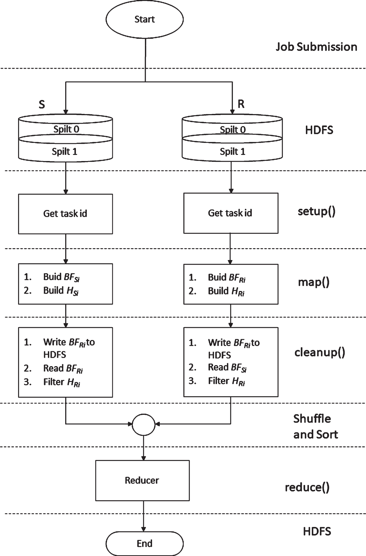
Reduce-side Bloom join in [9] requires two MapReduce jobs to implement the join operation. We introduce the Adaptive Bloom Join algorithm which creates the Bloom filter and performs the join operation within a single MapReduce job. To make this possible without any prior modifications to the Hadoop architecture, we enable the worker nodes to communicate during a running job through the Hadoop Distributed File System (HDFS) with the use of Mapper’s functionalities. Each instance of the Mapper class has four methods, setup(), map(), cleanup() and run(). The adaptive Bloom join utilizes the setup() and cleanup() methods to initialize important parameters and to write the local filters to HDFS, respectively. In addition, our approach utilizes the map() method to extract the key/value pairs and to construct the local filters. Figure 1 shows the flow diagram of a join operation between R and S using the adaptive Bloom join.

Fig. 1

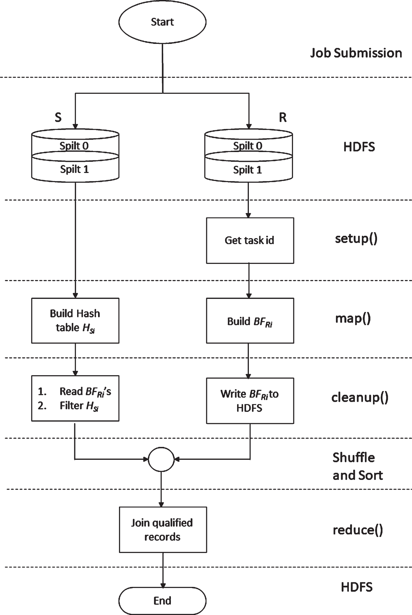
Flow diagram of adaptive Bloom join.

The following steps describe the implementation of the adaptive Bloom join algorithm.

Job submission: Once the user submits the job, the MapReduce framework creates mp₁ map tasks for S and mp₂ map tasks for R and r reduce tasks.

Map phase setup: We use the task number as a label for each local Bloom filter BF_Ri. The main benefit of uniquely labeling the local filters is to facilitate the process of storing and loading them to/from HDFS. In Fig. 1, a Bloom filter of R is constructed to eliminate redundant records in S. Therefore, the setup method of S is skipped. In the setup method of R, each mapper retrieves the map task id using the job configuration object and stores the last part of the task id.

Map phase map: In the map method of R, each mapper iterates through each record of the input split R_i of R, extracts the key/value pair, and outputs a< key, tag value>pair. Then, each mapper adds the hash value of the key to the local filter BF_Ri and writes the intermediate results to the local disk of the worker node. On the other side, each mapper of S constructs a hash table H_Si for the input split S_i of S. All mappers of S defer writing the intermediate results to the cleanup method in order to eliminate the redundant records of S.

Map phase cleanup: Each mapper of R writes its local filter BF_Ri on a predefined directory D_R in HDFS. To avoid any conflict, a unique name, Filter_X, is used to label each local filter, where X refers to the last part of the task id which is extracted in the setup phase. Then, each mapper of R creates an empty file Ack_X to acknowledge mappers of S that Filter_X has been successfully written to HDFS. In the opposite side, each mapper of S continuously probes D_R for the acknowledgment files, and once a new Ack_X is written, it reads the corresponding filter file. This process is repeated until all filter files are read. Then, each mapper of S merges the local filters into one global filter to eliminate redundant records in H_Si. Finally, the filtered intermediate results are written to the local disk of the worker node.

Shuffle and Sort: The MapReduce framework partitions the intermediate results of each mapper into r partitions and sends each partition to the corresponding reducer for aggregation and sorting.

Reduce phase: For each join key, the reduce function separates the input records based on their tag into two sets and buffers the records of each set. Then, it performs a cross-product between the buffered records and writes the join result to HDFS.

The adaptive bloom join algorithm facilitates the processes of creating the Bloom filters on one side and reading them on the other side. Figure 2 shows an example of an equijoin operation using adaptive Bloom join. In this example, the mapper of R builds a local Bloom filter ‘Filter0’ and writes it to a predefined directory D_R in HDFS, as well as an acknowledgment file Ack₀. Then, the R side mapper outputs the tagged key/value pairs. In the S side, each mapper verifies if the acknowledgment file exists in the predefined directory D_R, if so, it reads the local filter and eliminates redundant records in the input data. Finally, the intermediate records are sorted and shuffled and eventually sent to the reducers to produce the join result.

Fig. 2

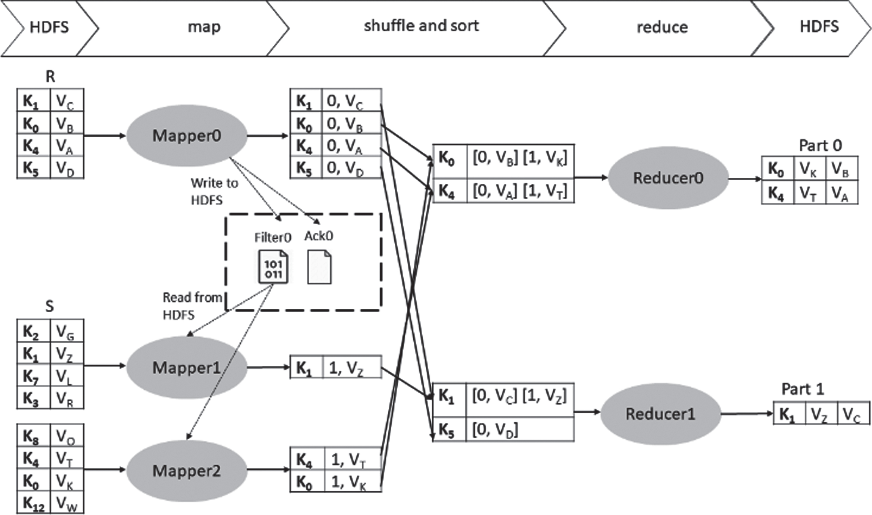
Example of adaptive Bloom join.

Compared to Bloom join in [9], the adaptive Bloom join eliminates the cost of implementing the first job that constructs the Bloom filter. And compared to join processing using Bloom filter in [13], our approach is implemented in the MapReduce framework without any prior modifications to its architecture.

3.2 Algorithm₂: Semi-adaptive intersection bloom join

The intersection Bloom join [14, 15] significantly improves the join performance by eliminating redundant records in both tables using the intersection filter. However, the preprocessing is more involved compared to other Bloom joins. Therefore, we introduce the Semi-Adaptive Intersection Bloom Join algorithm to alleviate this problem. The introduced algorithm is implemented in two MapReduce jobs. The first job runs a full MapReduce job to construct a Bloom filter BF_S for table S. Each mapper builds a local filter for the input split S_i of S. Then, the local filters are eventually fed to a reducer, which in turn merges them into one global filter BF_S. The second MapReduce job constructs a Bloom filter BF_R for table R on-the-fly and performs the join operation after eliminating redundant records in both tables. Figure 3 shows the flow diagram of the second MapReduce job.

Fig. 3

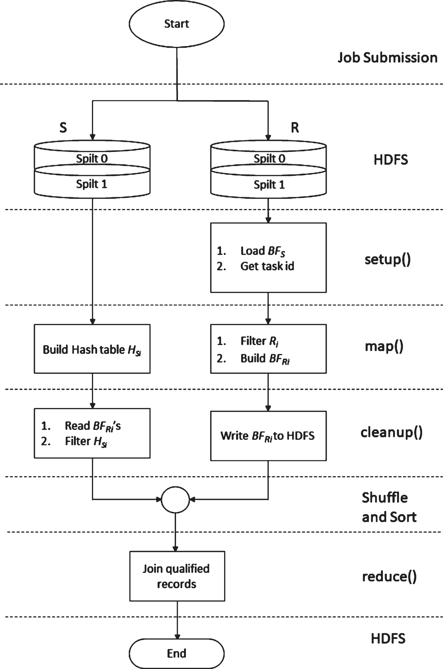
Flow diagram of semi-adaptive intersection Bloom join.

The following steps describe the implementation of the second MapReduce job.

Job submission: The MapReduce framework creates mp₁ map tasks for S and mp₂ map tasks for R and r reduce tasks. Then, it copies the configuration files of the job in addition to the Bloom filter BF_S, which is created in the first job, to all tasks.

Map phase setup: Firstly, the BF_S is loaded into the cache memory of every node executing map tasks of R. Secondly, the Bloom filter of R is constructed on-the-fly. Therefore, we need to retrieve the task id in order to uniquely label each local filter of R, as in adaptive Bloom join. On the other side, mappers of S neither construct a local filter nor load any cached filter. Therefore, the setup method of S is skipped.

Map phase map: Firstly, each mapper of R iterates through each record of the input split R_i of R and extracts the key/value pair. Then, it verifies if the extracted pair is a joinable record or not as a result of testing the membership of the extracted key in BF_S. If that is the case, then the mapper tags the extracted pair according to its source. Otherwise, the record is disregarded. Secondly, the hash values of the joinable keys are added to the local Bloom filter BF_Ri. Finally, the intermediate results are written to the local disk of the worker nodes in preparation for the reduce phase. On the other side, each mapper of S iterates through each record of the input split S_i of S and extracts the key/value pair. Then, it adds each key/value pair to an in-memory hash table H_Si.

Map phase cleanup: In the R side, the cleanup method of each mapper writes the constructed local filter BF_Ri to a predefined directory D_R in HDFS, as well as the acknowledgment files. Filter_X and Ack_X are the naming convention of the local filters and acknowledgment files, respectively. On the other side, the cleanup method of S continuously probes the directory D_R for the acknowledgment files, and once a new one is written, it reads the corresponding filter file. Once all filters are loaded, the cleanup method merges them into one global filter. Finally, it iterates through each record of the in-memory hash table H_Si and outputs a< key, tag value>pair for each joinable record.

Shuffle and Sort: The MapReduce framework partitions and sorts the intermediate results. Then, it sends each partition to the corresponding reducer.

Reduce phase: Records from both tables are joined according to their key and the join result is written to HDFS.

The semi-adaptive intersection Bloom join filters out redundant records in both tables before entering the reduce phase. Figure 4 shows an example of an equijoin operation using the introduced algorithm. In this example, firstly, the R side mapper uses the global filter of S table, which is created in an independent MapReduce job, to eliminate redundant records in R. The rest of the implementation flows exactly as in the description of Fig. 2. Compared to the intersection Bloom join [14, 15], the semi-adaptive intersection Bloom join reduces the cost of preprocessing and increases the cost of processing in the join job. However, the reduced I/O cost in the preprocessing job overcomes the cost of the extra processing in the join job.

Fig. 4

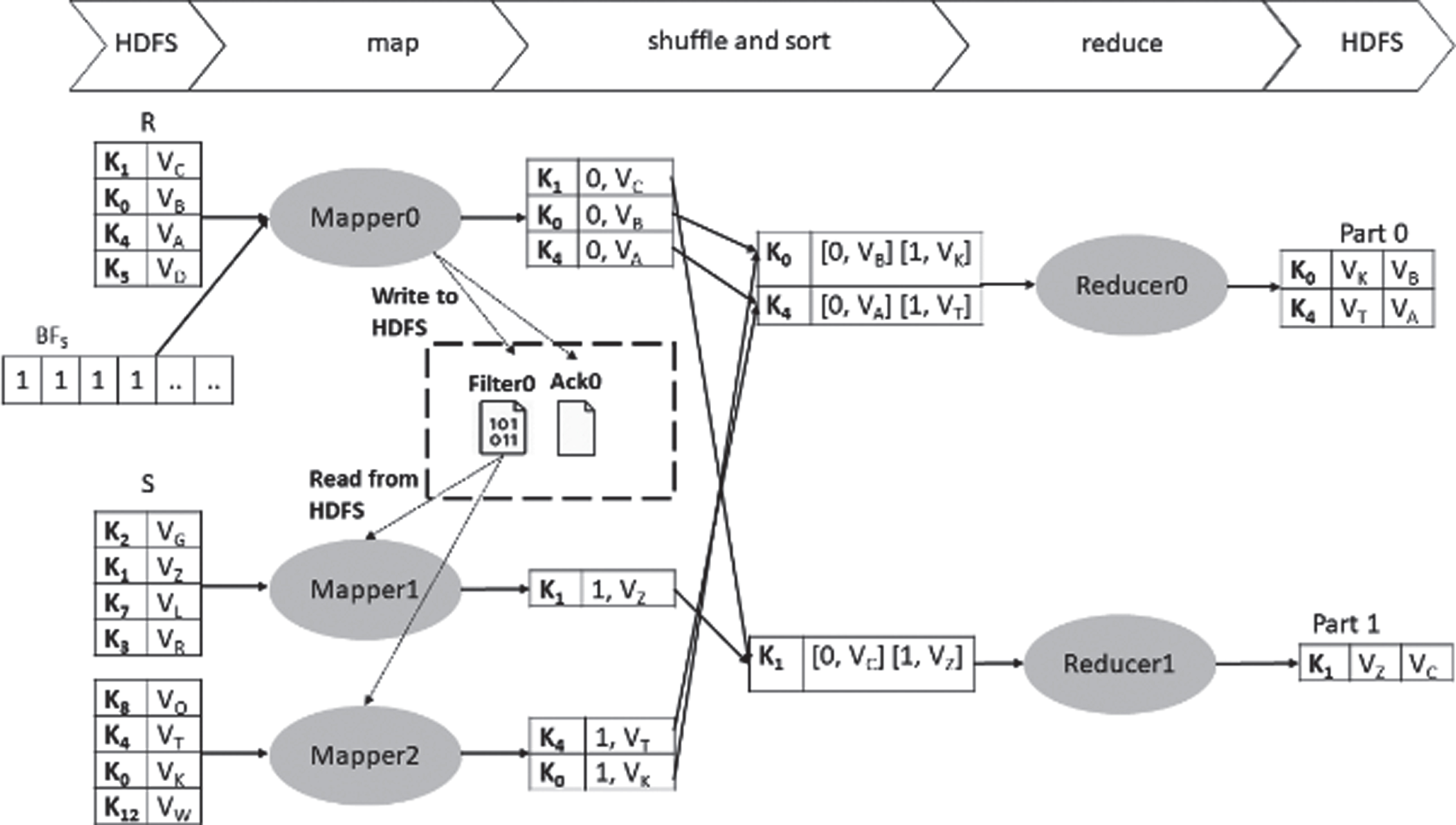
Example of semi-adaptive intersection Bloom join.

3.3 Algorithm₃: Adaptive intersection bloom join

To eliminate the cost of the preprocessing job in semi-adaptive intersection Bloom join, we introduce the Adaptive Intersection Bloom Join algorithm. It constructs Bloom filters for both tables and performs the join operation within a single MapReduce job. The local Bloom filters of both tables are constructed in the map method and interchanged in the cleanup method. Figure 5 shows the flow diagram of the introduced algorithm.

The following steps describe the implementation of the algorithm.

Job submission: The MapReduce framework creates mp₁ map tasks for S and mp₂ map tasks for R and r reduce tasks. Then, it copies the configurations files to all tasks.

Map phase setup: In both sides S and R, the setup method retrieves the tasks id and uses the last part of the task id to label the local filter.

Map phase map: Each mapper of R iterates through each record of the input split R_i of R and extracts the key/value pair. Then, it adds the hash value of the extracted key to the local filter BF_Ri and adds the hash value of the extracted key/value pair to the hash table H_Ri. The same logic is applied on the other side, the map method of S constructs a local Bloom filter BF_Si and a hash table H_Si for each input split S_i of S.

Map phase cleanup: The same logic is applied in both sides. Firstly, the cleanup method of each mapper writes the local filter, BF_Ri or BF_Si, and the corresponding acknowledgment file Ack_X to D_R or D_S in HDFS. These directories are predefined, and each side is only allowed to write to its corresponding directory. Secondly, the cleanup method continuously searches for the existence of the acknowledgment files in the opposite directory (D_R or D_S), and once a new file is written, it reads the corresponding filter file. Once all filters are read, the cleanup method merges them into one global filter, BF_R or BF_S. Finally, it iterates through each record of the hash table H_R or H_S and transfers the joinable records to the reduce phase.

Shuffle and Sort: The intermediate results are sorted and written to the local disk of the worker nodes. Then, the MapReduce framework sends them to the reducers.

Reduce phase: Records from both tables are joined according to their key and the join result is written to HDFS.

Fig. 5

Flow diagram of adaptive intersection Bloom join.

Figure 6 shows an example of an equijoin operation using the adaptive intersection Bloom join, where D_R and D_S are directories in HDFS used to store the local filters and acknowledgment files of R and S, respectively. The mapper of R side builds a local filter ‘Filter0’ for the input split and writes it to D_R, as well as the acknowledgment file Ack₀. Concurrently, mappers of S side build the local filters ‘Filter1’ and ‘Filter2’ and write them to D_S, as well as the acknowledgment files Ack₁ and Ack₂. Then, each mapper reads the local filters of the other side and use it/them to eliminate redundant records in its input spilt. Finally, the filtered intermediate records are sent to the reducers to produce the join result.

Fig. 6

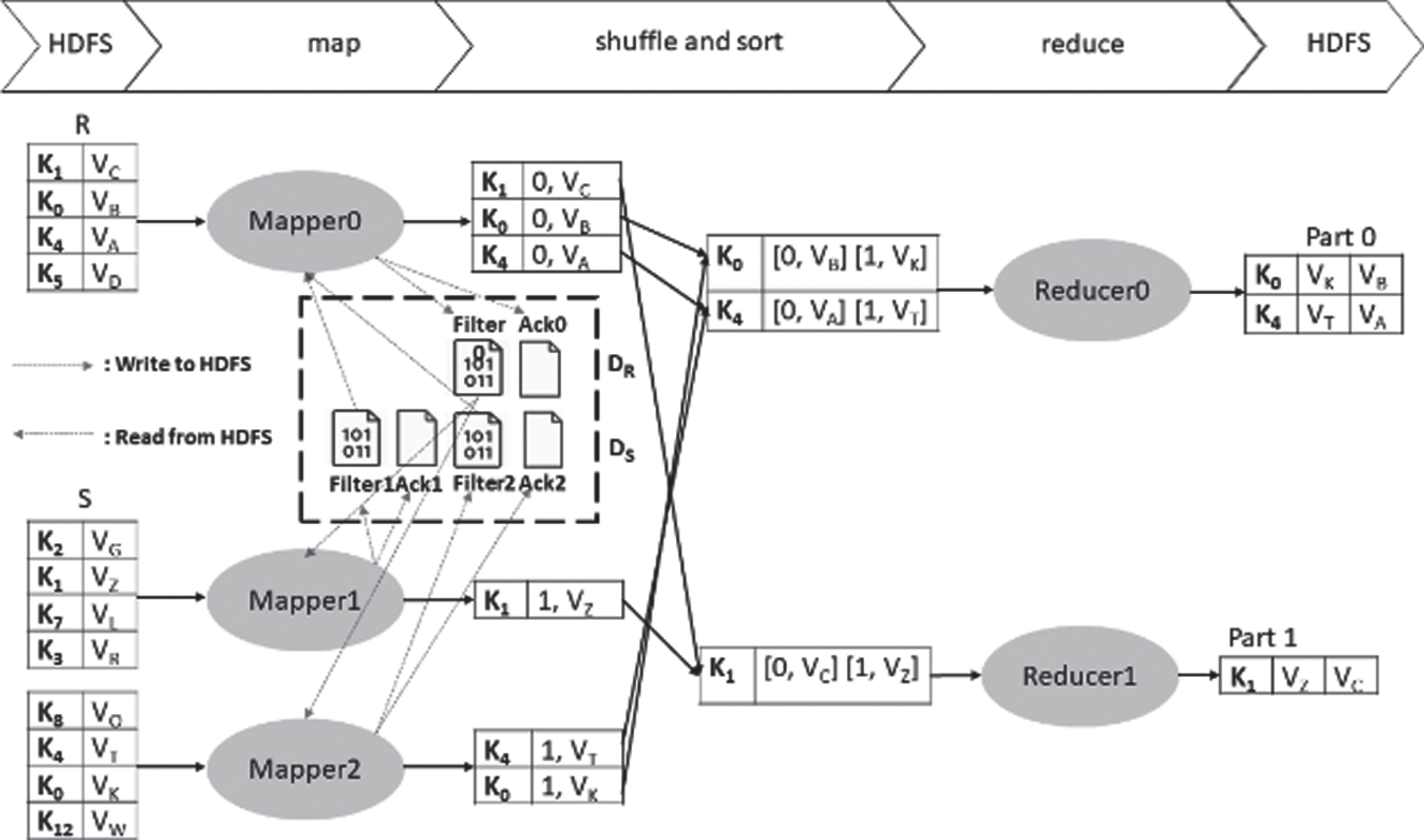
Example of adaptive intersection Bloom join.

Communicating through HDFS facilitates the processes of writing and reading the local filters within one MapReduce job. Compared to the intersection Bloom join [14, 15], the adaptive intersection Bloom join reduces the total amount of transferred data between mappers and reducers and eliminates the cost of the preprocessing job.

3.4 Bloom filters construction strategies

The introduced adaptive filter-based join algorithms utilize HDFS to distribute the local filters between mappers of the input datasets. However, a network bottleneck might occur if the size of these filters or the number of map tasks is relatively large. In this subsection, we introduce two strategies to dynamically compute and distribute the local filters and discuss their efficiencies. A cost analysis of these strategies is presented in the next section.

Given an input dataset R, we can compute the size of the Bloom filter BF_R, denoted as m_R, using Equation (1) [41], where n_total is the total number of join keys and p is the false positive probability. $\begin{matrix} m_{R} = - \frac{ln p}{(ln 2)^{2}} \times n_{total} \end{matrix}$ (1)

Strategy₁: Each mapper of R constructs a local filter and writes it to a predefined directory D_R in HDFS. On the other hand, each mapper of S reads the written filters and merges them into one global filter. The size of each local filter is constructed based on the total number of keys of R and the false probability rate, as in Equation (1). To increase the efficiency, we could alter the block size of R to be larger than that of S in order to guarantee the early assignment of R‘s map tasks. Strategy₁ is used in the description of the introduced algorithms in the previous subsections.

Strategy₂: Each mapper of R constructs a local filter and writes it to a predefined directory D_R in HDFS. Once all filters are written, the last assigned map task of R reads the written filters and merges them into one global filter. Then, it writes the global filter file along with an acknowledgment file to D_R. In the S side, each mapper continuously probes for the acknowledgment file in directory D_R, and once it is written, each mapper of S reads the global filter file. In this way, mappers of S read only one filter. The local filters and the global filter used in this strategy₂ have the same size.

By comparing strategy₂ to strategy₁, it is clear that strategy₂ reduces the total number of I/O operations. On the other hand, it requires extra time to process the global filter. There is a tradeoff between these two measures. If the size of the input datasets is relatively large, then strategy₂ becomes more efficient than strategy₁, because the decrease in the total number of I/O operations overcomes the increase in the processing time. Otherwise, strategy₁ becomes more efficient than strategy₂.

4 Cost analysis of filter-based join algorithms

Consider an equijoin operation between R and S in the MapReduce environment. This section presents the cost analysis of the state-of-the-art join algorithms: Standard Repartition Join, Bloom Join, and Intersection Bloom Join, respectively. In addition, we present the cost analysis of the introduced join algorithms: Adaptive Bloom Join, Semi-Adaptive Intersection Bloom Join, and Adaptive Intersection Bloom Join, respectively. The naming convention for representing the join algorithms is provided in Table 1.

Table 1
Abbreviations for representing the join algorithms

Abbreviation Algorithm

SRJ Standard Repartition Join

BJ Bloom Join

IBJ Intersection Bloom Join

ABJ Adaptive Bloom Join

SAIBJ Semi-Adaptive Intersection Bloom Join

AIBJ Adaptive Interaction Bloom Join

Abbreviation	Algorithm
SRJ	Standard Repartition Join
BJ	Bloom Join
IBJ	Intersection Bloom Join
ABJ	Adaptive Bloom Join
SAIBJ	Semi-Adaptive Intersection Bloom Join
AIBJ	Adaptive Interaction Bloom Join

4.1 Cost model

We adapt the cost model introduced in [42]. Table 2 summarizes the parameters of the model. The cost of the mentioned algorithms is analyzed under the same assumption of the introduced cost model, which states that the execution time is dominated by I/O operations, such as reading, writing, and copying. All costs, denoted by small c, are measured in seconds per page and the total costs, denoted by capital C, are measured in seconds. The total cost of a two-way equijoin operation using MapReduce is given in Equation (2).

$\begin{matrix} C_{Join} = C_{pre} + C_{read} + C_{sort} + C_{tr} + C_{write} \end{matrix}$ (2)

Table 2

Parameters of the cost model

Parameter	Description
\|R\|	The size of R in Bytes
\|S\|	The size of S in Bytes
\|D\|	The size of intermediate data in Bytes
\|O\|	The size of the output data in Bytes
B+1	The size of the sort buffer in pages
BF_R	The Bloom filter of R
BF_S	The Bloom filter of S
IBF	The intersection Bloom filter, IBF = BF_R ∩ BF_S
m	The size of the Bloom filter in bits (all filters, BF_R,
	BF_S, and IBF, have the same size)
mp ₁	The number of map tasks of S
mp ₂	The number of map tasks of R
mp	The total number of map tasks mp=mp₁+mp₂
n	The number of worker nodes
c_l	The cost of reading/writing data locally
c_r	The cost of reading/writing data remotely
c_t	The cost of transferring data from one node to another
C_pre	The total cost of the preprocessing jobs
C_read	The total cost of reading the input datasets

where:

C_read = c_r · |R| + c_r · |S|

C_sort = c_l · |D|·2 · (log _B|D| - log _B (mp) + log _B (mp)) as in [42].

C_tr = c_t · |D|

C_write = c_r · |O|

The additional component C_pre depends on the amount of I/O operations involved in the preprocessing job of the algorithm. For instance, the C_pre of SRJ is equal to zero. The two components C_read and C_write are fixed regardless of the join algorithm, since they only depend on the size of the input datasets, |R| and |S|, and the size of the join output |O|. The remaining components, C_sort and C_tr, strongly influence the total cost of a join algorithm, because they depend on the size of intermediate data |D|. Therefore, an optimized join algorithm should minimize the total amount of intermediate data.

4.2 Cost comparison

In this subsection, we analyze the cost of the join algorithms in terms of |D|, C_pre, and the cost of any additional phase. We set the cost of SRJ as the base cost to highlight the effect of filtering. Since ABJ is an optimization of BJ, and SAIBJ and AIBJ are optimizations of IBJ, we divide the filter-based join algorithms into two categories: BJ and ABJ in the first category and IBJ, SAIBJ, and AIBJ in the second category. We denote the following symbols for the below parameters.

δ _R : the ratio of joined records of R with S.

δ _S : the ratio of joined records of S with R.

p(R): the false positive probability of BF_R.

p(R, S): the false positive probability of the intersection Bloom filter, IBF = BF_R ∩ BF_S.

Standard Repartition Join (SRJ): The preprocessing cost of SRJ is equal to zero and the total amount of intermediate data is equal to the size of the input datasets, R and S. $\begin{matrix} C_{pre} = 0 \end{matrix}$ (3) $\begin{matrix} | D |_{SRJ} = | R | + | S | \end{matrix}$ (4)

Category₁: The I/O operations in the preprocessing job of BJ involve the following: reading the input dataset R, writing the local filters to the local disk of the worker nodes, transferring them to the reducers and writing the merged filter to HDFS. The join job eliminates the cost of transferring the redundant records of S. Equations (5) and (6) compute the total preprocessing cost and the total amount of intermediate data of BJ. $C_{{pre}_{B} J} = c_{r} \cdot | R | + c_{l} \cdot m \cdot {mp}_{1} + c_{t} \cdot m \cdot {mp}_{1} + c_{r} \cdot m$ $\begin{matrix} C_{{pre}_{BJ}} = c_{r} \cdot | R | + (c_{l} + c_{t}) \cdot m \cdot {mp}_{1} + c_{r} \cdot m \end{matrix}$ (5) $\begin{matrix} | D |_{BJ} = | R | + δ_{R} \cdot | S | + (1 - δ_{R}) \cdot p (R) \cdot | S | \end{matrix}$ (6)

ABJ eliminates the cost of preprocessing, however, it adds an extra phase to write and read the local filters of R to/from HDFS, respectively, denoted as C_f (cost of the filters). We ignore the computation of the I/O operations of strategy₁ and strategy₂ that involve writing and checking the acknowledgment files because these are empty files and the cost of their creation is almost negligible compared to the total cost. We compute C_f in the worst-case scenario, assuming that all map tasks of S read the local filters from HDFS remotely. However, in real clusters, the introduced join algorithms benefit from the file replication property of MapReduce. The I/O operations of C_f using strategy₁ involve writing the local filters of R and reading them on S side. Equation (7) computes the cost of this phase. $C_{f_ABJ_strategy 1} = c_{r} \cdot m \cdot {mp}_{2} + c_{r} \cdot m \cdot {mp}_{1} \cdot {mp}_{2}$ $\begin{matrix} C_{f_{{ABJ}_{strategy 1}}} = c_{r} \cdot m \cdot {mp}_{2} (1 + {mp}_{1}) \end{matrix}$ (7)

The I/O operations of C_f using strategy₂ involve writing the local filters of R, then, one map task of R reads them and write the global filter to HDFS. Finally, all map tasks of S read the global filter from HDFS. Equation (8) computes C_f of strategy₂. $\begin{matrix} C_{f_ABJ_strategy 2} = \\ c_{r} \cdot m \cdot {mp}_{2} + c_{r} \cdot m \cdot {mp}_{2} + c_{r} \cdot m + c_{r} \cdot m \cdot {mp}_{1} \end{matrix}$ $\begin{matrix} C_{f_ABJ_strategy 2} = c_{r} \cdot m \cdot (2 {mp}_{2} + {mp}_{1} + 1) \end{matrix}$ (8)

The size of intermediate data of ABJ is equal to that of BJ, given in (6). However, the cost of processing the filters is different. From Equations (5), (7), and (8) we can infer the following.

Lemma 1. Strategy₂ is more efficient than strategy₁ for all mp₁>2 and mp₂>2 because it minimizes the I/O operations of C_f. $\begin{matrix} C_{f_{{ABJ}_{strategy 2}}} < C_{f_{{ABJ}_{strategy 1}}} \\ {\forall {mp}_{1} > 2 and \forall {mp}_{2} > 2} \end{matrix}$ (9)

Proof. By comparing (7) and (8) we can deduce that: $\begin{matrix} 2 {mp}_{2} + {mp}_{1} + 1 < {mp}_{2} + {mp}_{1} \cdot {mp}_{2} \\ \begin{matrix} {mp}_{2} + {mp}_{1} + 1 < {mp}_{1} \cdot {mp}_{2} \\ {\forall {mp}_{1} > 2 andforall {mp}_{2} > 2} \end{matrix} \end{matrix}$ (10)

We hereby analyze the cost of the introduced join algorithms using strategy₂. To shorten the discussion and highlight the conclusion, we eliminate analyzing the cost using strategy₁.

Lemma 2. ABJ is more efficient than BJ for all m< (α * splitsize), where α<1. $\begin{matrix} C_{f_{ABJ}} < C_{{pre}_{BJ}} {\forall m < α \cdot splitsize} \end{matrix}$ (11)

Proof. By combining Equations (5) and (8), we get the following: $\begin{matrix} c_{r} \cdot m \cdot (2 {mp}_{2} + {mp}_{1} + 1) \\ < c_{r} \cdot | R | + (c_{l} + c_{t}) \cdot m \cdot {mp}_{1} + c_{r} \cdot m \end{matrix}$

By default, the split size is equal to 128MB. Therefore, |R| is approximately equal to the split size multiplied by the total number of mappers. Let g = c_t/c_l, and h=c_r/c_l. Then, by dividing the above inequality by c_l and by substituting the value of | R |, we get the following: $\begin{matrix} h \cdot m \cdot (2 {mp}_{2} + {mp}_{1} + 1) \\ < h \cdot splitzie \cdot {mp}_{2} + (1 + g) \cdot m \cdot {mp}_{1} + h \cdot m \\ m < \frac{h \cdot {mp}_{2}}{h \cdot (2 {mp}_{2} + {mp}_{1}) - (1 + g) \cdot {mp}_{1}} \cdot splitsize \\ \begin{matrix} m < α \cdot splitsize \end{matrix} \end{matrix}$ (12)

From inequalities (11) and (12), α is a constant coefficient that is less than one. It depends on the size of the input datasets and the characteristics of the cluster. However, in real clusters, the coefficient α could exceed one.

Category₂: The preprocessing of IBJ is more involved than that of BJ. On the other hand, the amount of intermediate data of IBJ is smaller than that of BJ, because IBJ filters out redundant records in both datasets. The preprocessing of IBJ involves reading R and S, writing a local filter for each input split, and transferring the local filters to the reducers. Then, the global filter is written in the reduce phase. Equations (13) and (14) compute the cost of the preprocessing job and the total amount of intermediate data of IBJ. $\begin{matrix} C_{{pre}_{I} BJ} = c_{r} \cdot | R | + c_{r} \cdot | S | + c_{l} \cdot m \cdot mp + \\ c_{t} \cdot m \cdot mp + c_{r} \cdot m \\ \begin{matrix} C_{{pre}_{IBJ}} = c_{r} \cdot | R | + c_{r} \cdot | S | \\ + (c_{l} + c_{t}) \cdot m \cdot mp + c_{r} \cdot m \end{matrix} \end{matrix}$ (13) $\begin{matrix} | D |_{IBJ} = δ_{S} \cdot | R | + (1 - δ_{S}) \cdot p (R, S) \cdot | R | \\ + δ_{R} \cdot | S | + (1 - δ_{R}) \cdot p (R, S) \cdot | S | \end{matrix}$ (14)

SAIBJ reduces the total cost of I/O operations in the preprocessing job compared to IBJ, since it only constructs the filter of R. On the other hand, it adds an extra phase C_f to construct the filter of S in the join job. Equations (15) and (16) compute the cost of the preprocessing job and the cost of the filters of SAIBJ. $\begin{matrix} \begin{matrix} C_{{pre}_{SAIBJ}} = c_{r} \cdot | R | + (c_{l} + c_{t}) \cdot m \cdot {mp}_{1} \\ + c_{r} \cdot m \end{matrix} \end{matrix}$ (15) $\begin{matrix} C_{f_{SAIBJ}} = c_{r} \cdot m \cdot (2 {mp}_{1} + {mp}_{2} + 1) \end{matrix}$ (16)

AIBJ completely eliminates the cost of preprocessing, however, it adds an extra cost C_f to the join job. The I/O operations in C_f involve creating the filters of R and S. Equation (17) computes the cost of filters of AIBJ. $\begin{matrix} C_{f_{A} IBJ} = c_{r} \cdot m \cdot (2 {mp}_{2} + {mp}_{1} + 1) \\ + c_{r} \cdot m \cdot (2 {mp}_{1} + {mp}_{2} + 1) \\ C_{f_{A} IBJ} = c_{r} \cdot m \cdot (3 {mp}_{1} + 3 {mp}_{2} + 2) \\ \begin{matrix} C_{f_{AIBJ}} = c_{r} \cdot m \cdot (3 mp + 2) \end{matrix} \end{matrix}$ (17)

The size of intermediate data of AIBJ and SAIBJ is equal to that of IBJ, which is given in Equation (14). From Equations (13 –17) we can infer the following.

Lemma 3. SAIBJ is more efficient than IBJ for all m< (α * splitsize), where α<1. $\begin{matrix} C_{{pre}_{SAIBJ}} + C_{f_{SAIBJ}} < C_{{pre}_{IBJ}} \\ {\forall m < α \cdot splitsize} \end{matrix}$ (18)Proof. By combining Equations (12), (14) and (15) and if g=c_t/c_l, and h=c_r/c_l, we get the following: $\begin{matrix} c_{r} \cdot | R | + (c_{l} + c_{t}) \cdot m \cdot {mp}_{1} + c_{r} \cdot m + c_{r} \cdot m \\ \cdot (2 {mp}_{1} + {mp}_{2} + 1) \\ < c_{r} \cdot | R | + c_{r} \cdot | S | + (c_{l} + c_{t}) \\ \cdot m \cdot mp + c_{r} \cdot m \end{matrix}$ $\begin{matrix} (c_{l} + c_{t}) \cdot m \cdot {mp}_{1} + c_{r} \cdot m \cdot (2 {mp}_{1} + {mp}_{2} + 1) \\ < c_{r} \cdot | S | + (c_{l} + c_{t}) \cdot m \cdot ({mp}_{1} + {mp}_{2}) \end{matrix}$

And by dividing the above inequality by c_l, we get the following: $\begin{matrix} h \cdot m \cdot (2 {mp}_{1} + {mp}_{2} + 1) \\ < h \cdot splitsize \cdot {mp}_{1} + (1 + g) \cdot m \cdot {mp}_{2} \\ m < \frac{h \cdot {mp}_{1}}{h \cdot (2 {mp}_{1} + {mp}_{2} + 1) - (1 + g) \cdot {mp}_{1}} \cdot splitsize \\ \begin{matrix} m < α \cdot splitsize \end{matrix} \end{matrix}$ (19)

Lemma 4. AIBJ is more efficient than IBJ for all m< (α * splitsize), where α<1. $\begin{matrix} C_{f_{AIBJ}} < C_{{pre}_{IBJ}} {\forall m < α \cdot splitsize} \end{matrix}$ (20)

Proof. By combining Equations (13) and (17) and if g = c_t/_l, and h = c_r/c_l, we get the following: $\begin{matrix} c_{r} \cdot m \cdot (3 mp + 2) < \\ c_{r} \cdot | R | + c_{r} \cdot | S | + (c_{l} + c_{t}) \cdot m \cdot mp + c_{r} \cdot m \\ c_{r} \cdot m \cdot (3 mp + 2) < \\ c_{r} \cdot splitsize \cdot mp + (c_{l} + c_{t}) \cdot m \cdot mp + c_{r} \cdot m \end{matrix}$

And by dividing the above inequality by c_l, we get the following: $\begin{matrix} m < \frac{h \cdot mp}{h \cdot (3 mp + 1) - (1 + g) \cdot mp} \cdot splitsize \\ \begin{matrix} m < α \cdot splitsize \end{matrix} \end{matrix}$ (21)

In summary, the introduced algorithms ABJ, SAIBJ, and AIBJ reduce the total cost of the join operation compared to BJ and IBJ. Theoretically, they have been proven to be more efficient than the state-of-the-art filter-based joins for all filter sizes less than a certain fraction (α) of the split size. Therefore, ABJ is a better choice than BJ, SAIBJ, and AIBJ are better choices than IBJ. However, if the join ratio is relatively high, then SRJ outperforms the filter-based joins, because the cost of constructing and distributing the filters becomes relatively significant.

5 Experimental results and discussion

In this section, we present experimental results of the state-of-the-art filter-based joins and our algorithms. We implemented four tests to capture the performance in different aspects of the join operation. Test₁ and Test₂ examined the effect of varying the input size and join ratio, respectively. Test₃ was dedicated to measure the performance of AIBJ, since the algorithm is restricted to the available resources in the cluster. Finally, Test₄ examined the effect of varying the Bloom filter size. The performance is measured in terms of the total execution time and the total amount of I/O data.

Cluster Environment. All experiments were run on a cloud-based cluster, IBM Analytics Demo Cloud. It is a high-performance cluster that demonstrates the advantages of parallelized processing of big datasets. It consists of four nodes, one master node and three worker nodes. Table 3 summarizes their characteristics. The cluster supports multiple services such as Apache Hadoop and Apache Spark and managed by Apache Ambari. The Hadoop version is 2.7.1 and the Ambari version is 2.1.0. The default configurations of the cluster were maintained, where the block size was 128MB, the block replication factor was three, the dedicated memory for sorting data was 819MB, the I/O buffer was 128KB and the JVMs heap-size was 1638MB. Furthermore, the total number of reduce tasks was set to four. Each worker node can simultaneously run up to 20 tasks.

Table 3
Cluster characteristics

Node Role Memory CPU Hard Disk

Node ₀ NameNode/ResourceManager 252GB 32vCPU –

Node ₁ DataNode/NodeManager 63GB 32vCPU 17TB

Node ₂ DataNode/NodeManager 63GB 32vCPU 17TB

Node ₃ DataNode/NodeManager 63GB 32vCPU 28TB

Node	Role	Memory	CPU	Hard Disk
Node ₀	NameNode/ResourceManager	252GB	32vCPU	–
Node ₁	DataNode/NodeManager	63GB	32vCPU	17TB
Node ₂	DataNode/NodeManager	63GB	32vCPU	17TB
Node ₃	DataNode/NodeManager	63GB	32vCPU	28TB

Datasets. The self-join datasets of the Purdue MapReduce Benchmark Suite [43] were used in the experiments. The Purdue MapReduce benchmark, called “Puma”, represents a wide variety of MapReduce applications with low/high computing requirements and low/high shuffle volumes. Two datasets, namely Dataset₁ and Dataset₂, with an equal size were used in the implementation of the join operation. The maximum number of attributes in each dataset is 39, and the string length of each attribute is equal to 19 characters. The attributes of each record are separated by a comma and each record ends with a new line. The first attribute of Dataset₁ is a foreign key that refers to the sixth attribute of Dataset₂. We used the following query in the execution of the join algorithms.

Select *

From Dataset₁(A₀,..., A₂₀) d₁,

Dataset₂(A₀,..., A₂₀) d₂

Where d₁.A₀=d₂.A₅

The above query merges the first 21 attributes of Dataset₁ and Dataset₂ based on an equijoin condition; whenever the first attribute A₀ of Dataset₁ matches with the sixth attribute A₅ of Dataset₂.

5.1 Test₁: Scalability

We used three sets of input Set₁, Set₂, and Set₃ with respective sizes 30GB, 80GB, and 120GB to examine the scalability of BJ, IBJ, ABJ, and SAIBJ. Table 4 summarizes the characteristics of the input datasets. To highlight the effect of varying the input size, the join ratio of this test was set to 0.1%.

Table 4
Test₁ input datasets

Input Dataset ₁ Dataset ₂

Set ₁ size 15GB 15GB

# of records 37,571,850 37,428,177

Set ₂ size 40 40

# of records 102,322,416 101,983,585

Set ₃ size 60GB 60GB

# of records 161,030,087 161,029,465

Input	Dataset ₁	Dataset ₂
Set ₁	size	15GB	15GB
	# of records	37,571,850	37,428,177
Set ₂	size	40	40
	# of records	102,322,416	101,983,585
Set ₃	size	60GB	60GB
	# of records	161,030,087	161,029,465

In BJ and ABJ, the Bloom filter was constructed for Dataset₂. In SAIBJ, the Bloom filters of Dataset₁ and Dataset₂ were constructed in the first and second jobs, respectively. In order to maximize the efficiency of the filtering process, we specified the sizes of the Bloom filters according to the cardinality of the join key values of the input datasets and chose the most appropriate size with the smallest false positive probability. Table 5 shows the characteristics of the Bloom filters; where m is the size of the filter, k is the number of hash functions, n is the join key cardinality, m/n is the number of bits allocated for each key, and p is the false positive probability. The hash function type used in all filters was MurmurHash, which is a widely used hash function.

Table 5

Bloom filters parameters of Test₁

Sets	m (bit)	k	n	m/n	p
Set ₁	339038	7	15128	22	0.0001
Set ₂	517162	8	17498	29	0.00001
Set ₃	770955	8	26085	29	0.00001

The following shows the comparison of the experimental results.

Total Execution Time: Figure 7 shows the total execution time of BJ, ABJ, IBJ, and SAIBJ. Looking at ABJ and BJ, the total execution time of ABJ is less than that of BJ by percentages of 28%, 27%, and 34% for Set₁, Set₂, and Set₃, respectively. As the input size increases, the difference between the total execution time of ABJ and that of BJ increases as well. This is because of the increase in the I/O cost of the preprocessing job of BJ. The same is true when comparing SAIBJ to IBJ. The total execution time of SAIBJ is less than that of IBJ by percentages of 23%, 27%, and 24% for Set₁, Set₂, and Set₃, respectively. Although SAIBJ requires a preprocessing job like IBJ, its preprocessing I/O cost is minimized compared to that of IBJ. Therefore, SAIBJ has less total execution time than IBJ. Briefly, the dynamic creation of Bloom filter in ABJ and SAIBJ outperforms the static creation of Bloom filter in BJ and IBJ by average reductions of 30% and 25%, respectively.

Fig. 7

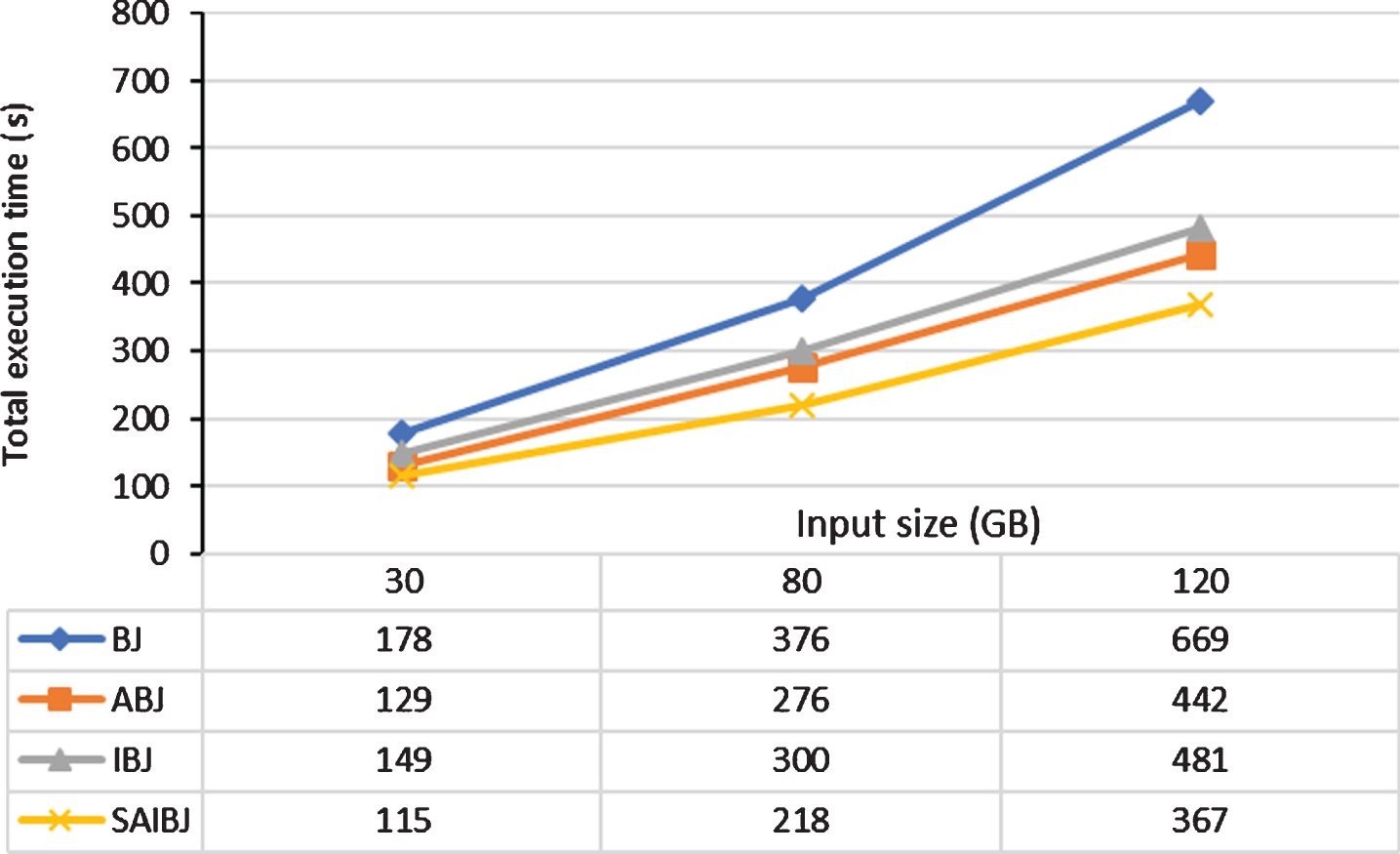
The total execution time of filter-based joins with varying the input size (Set₁, Set₂, Set₃).

Total Amount of I/O Data: The I/O operations play a major role in evaluating the performance of the join algorithms. Minimizing I/O operations improves the join performance and vice versa. We calculated the total amount of I/O data using the provided job counters, number of bytes read and number of bytes written locally or remotely. Figure 8 shows the total amount of I/O data of ABJ, BJ, SAIBJ, and IBJ. It can be noted that the differences between the total amount of I/O data of the existing approaches and that of the introduced approaches are approximately equal to the size of one input dataset for each set. For instance, in Set₂, the difference between the total amount of I/O data of BJ and that of ABJ, and the difference between the total amount of I/O data of IBJ and that of SAIBJ, are both approximately equal to 40GB. What is worth noting is that increasing the input size results in increasing the total difference between their total amount of I/O data. This will improve the performance of the introduced algorithms ABJ and SAIBJ. Concisely, by virtue of the dynamic creation of the Bloom filter in ABJ and SAIBJ, the total amount of I/O data is minimized by percentages of 18% and 25% compared to BJ and IBJ, respectively.

Fig. 8

Total amount of I/O of filter-based joins with varying the input size (Set₁, Set₂, Set₃).

5.2 Test₂: Join Ratio

In this test, we examined the effect of varying the join ratio of the input datasets on the performance of the filter-based joins. The total size of the input datasets was 30GB. We used MapReduce to tune the join ratio of the input datasets. Then, the algorithms were executed multiple times with different join ratios. Precisely, the join ratios were: 0.01%, 0.1%, 1%, and 2%. The following shows the comparison of the experimental results.

Total Execution Time: Figure 9 shows the total execution time of the filter-based joins with varying the join ratio. It is clearly noted that increasing the join ratio results in increasing the total execution time. Looking at ABJ and BJ, the difference between the total execution time of ABJ and that of BJ for each join ratio is within a range of 60 seconds. Therefore, we can deduce that increasing the join ratio mainly affects the shuffle time and the reduce time. Similarly, the difference between the total execution time of SAIBJ and that IBJ is approximately within a fixed range.

Fig. 9

Total execution time of filter-based joins with varying the join ratio.

Total amount of I/O Data: Increasing the join ratio affects the size of the intermediate data and the size of the join result. That is, large join ratios result in large amount of I/O data. Figure 10 depicts the effect of increasing the join ratio on the total amount of I/O data of the algorithms. ABJ and SAIBJ reduce the total amount of I/O data compared to BJ and IBJ, respectively, by a steady value that is approximately equal to 15GB. Therefore, we can conclude that varying the join ratio has the same effect on all join algorithms.

Fig. 10

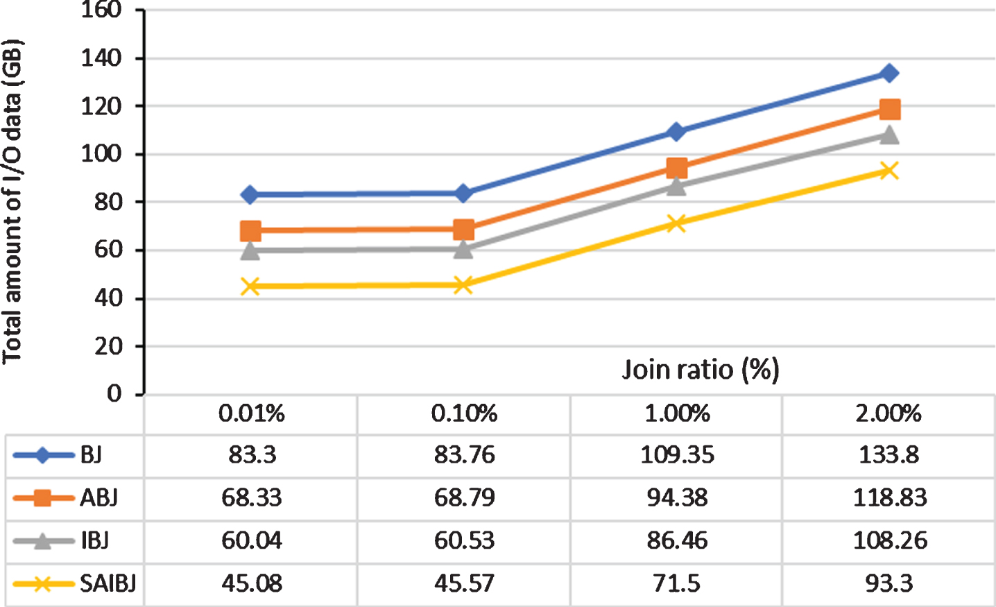
Total amount of I/O data of filter-based joins with varying the join ratio.

5.3 Test₃: Adaptive Intersection Bloom Join

AIBJ requires all map tasks to be executed at the same time. If at least one map task of AIBJ is waiting for other map tasks of the same job to release some resources, then AIBJ will not complete execution. In order to avoid this deadlock, we should consider the available resources in the cluster and the number of map tasks of a MapReduce job. Therefore, we dedicated Test₃ according to the capacity of resources in our cluster. Table 6 shows the characteristics of the input datasets used in this test. The performance of AIBJ was compared to that of IBJ according to the same metrics used in the previous tests. As in Test₁, the Bloom filter size was chosen according to the cardinality of the join key values and the false positive probability. The size of the Bloom filter was set to 16137 bits and the join ratio was set to 0.1%.

Table 6
Test₃ input datasets

Inputs Size Number of records

Dataset ₁ 2GB 5,367,350

Dataset ₂ 2GB 5,367,783

Total 4GB 10,735,133

Inputs	Size	Number of records
Dataset ₁	2GB	5,367,350
Dataset ₂	2GB	5,367,783
Total	4GB	10,735,133

The following shows the comparison of the experimental results.

Total Execution Time: Figure 11 shows the total execution time of AIBJ and IBJ. The advantage of eliminating the preprocessing job is clearly depicted in Fig. 11; the total execution time is reduced by a percentage of 34%. Although the join job of AIBJ consumes more time than that of IBJ, the payoff is evident in the preprocessing job.

Fig. 11

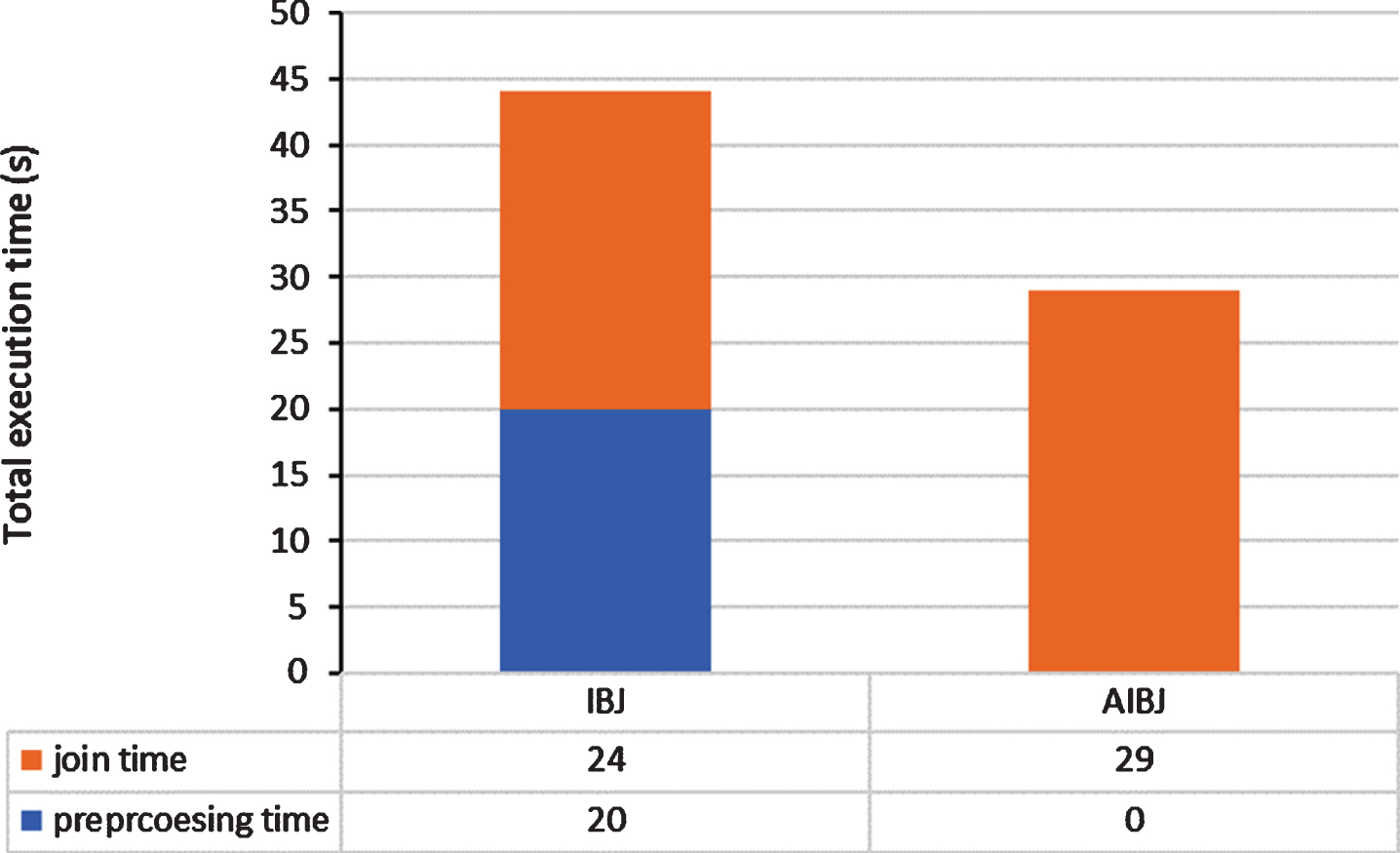
The total execution time of IBJ and AIBJ.

Total Amount of I/O Data: Figure 12 shows the total amount of I/O data of AIBJ and IBJ. The difference in the total amount of I/O data of AIBJ and that of IBJ is equal to the size of the input datasets (4GB). Since AIBJ eliminates the I/O cost of the preprocessing job, the total amount of I/O data is reduced by a percentage of 50% compared to IBJ.

Fig. 12

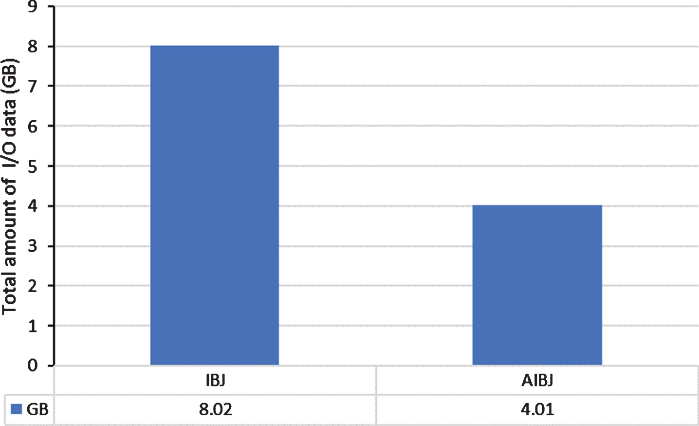
The total amount of I/O data of IBJ and AIBJ.

5.4 Test₄: Bloom filter size

The Bloom filter size plays a major role in the performance of the filter-based joins. Small filter sizes produce a high false-positive probability and, therefore, increase the number of intermediate records. In contrast, large filter sizes minimize the false positive probability, but they become inefficient in the processes of building and distributing the filters. Therefore, we should choose the optimal size that minimizes the false positive probability and can be efficiently distributed. In the previous tests, we considered these issues. However, in this test, the purpose is to examine the effect of increasing the filter size on the join performance and to find the threshold sizes of our algorithms that are analyzed in Lemma2, Lemma3, and Lemma4. In the experiments, the filter size varied from a minimum of 1MB to a maximum of 75MB. Furthermore, the input size was 30GB and the join ratio was set to 0.01%.

Figure 13 shows the total execution time of SRJ, BJ, ABJ, IBJ, and SAIBJ with varying the filter size. It can be clearly seen that increasing the filter size increases the total execution time of the algorithms, except SRJ. Looking at ABJ and BJ, ABJ exhibits a better performance than BJ for all filter sizes less than 75MB. Therefore, we can conclude that the threshold filter size of ABJ is approximately equal to 75MB. However, for filter sizes larger than 15MB, the filtering process in BJ becomes inefficient, and the same is true in ABJ for filter sizes larger than 25MB. This is because the performance of SRJ becomes better than ABJ and BJ. Turning to SAIBJ and IBJ, SAIBJ exhibits a better performance than IBJ for all filter sizes less than 15MB. Between 15MB and 50MB, both approaches exhibit a comparable performance. Then, SAIBJ begins to exhibit a better performance than IBJ for filter sizes larger than 50MB. This is because IBJ constructs an intersection filter, whereas SAIBJ constructs a pair of filters. However, for all filter sizes larger than 15MB, SRJ becomes the optimal choice.

Fig. 13

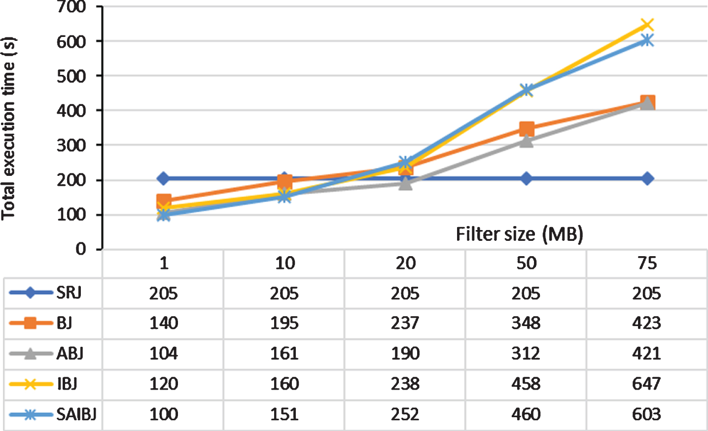
The total execution time of SRJ, BJ, ABJ, IBJ, and SAIBJ with varying the Bloom filter size.

In the evaluation of AIBJ, we used datasets with a total size of 4GB. Figure 14 shows the total execution time of AIBJ and IBJ with varying the filter size. As can be seen from Fig. 14, AIBJ exhibits a better performance than that of IBJ for all filter sizes. Therefore, the threshold filter size of AIBJ for this test is greater than 75MB.

Fig. 14

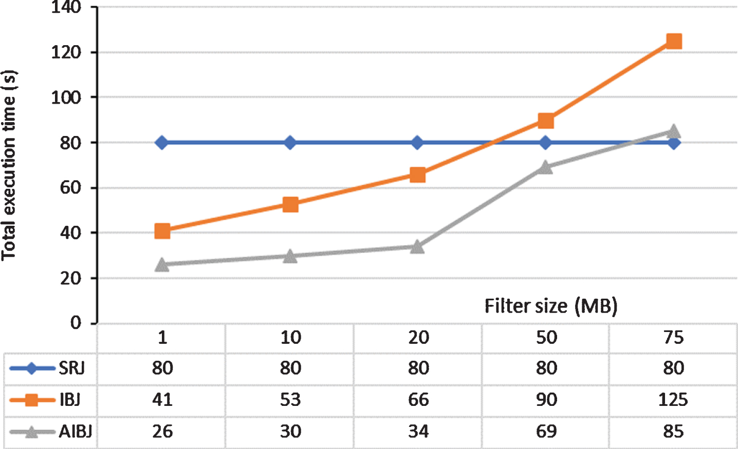
The total execution time of AIBJ and IBJ with varying the Bloom filter size.

5.5 Summary of discussion

It is quite evident from the results presented in Test₁ that ABJ and SAIBJ are scalable algorithms and outperform BJ and IBJ. Furthermore, the introduced algorithms improve the join performance as the input size increases. The results presented in Test₂ show that ABJ and SAIBJ steadily outperform BJ and IBJ with varying the join ratio. This is because increasing the join ratio only affects the shuffle time and the reduce time. On the other hand, increasing the join ratio decreases the efficiency of the filtering process. In Test₃, AIBJ outperforms IBJ, since it eliminates the I/O cost of preprocessing. The results of Test₄ show that ABJ, SAIBJ, and AIBJ are more efficient than BJ and IBJ for all filter sizes that enable the filtering process to outperform SRJ. What is worth noting is that as the filter size increases, the performance of SAIBJ and IBJ degrades faster than that of ABJ and BJ. This is because the latter approaches build a filter for only one input dataset.

In summary, the filtering process can boost the performance of a join query. SRJ sends all records from both datasets to the reduce phase. BJ and ABJ send all records from one dataset and the relevant records to the join operation from the other dataset. IBJ, SAIBJ, and AIBJ send only the relevant records to the join operation from both datasets. Table 7 shows the number of intermediate records for each join algorithm executed in Test₁ in addition to SRJ. Figure 15 shows their respective total execution time. SRJ has the largest execution time, while SAIBJ has the smallest execution time. As the input size increases, the performance of the filter-based joins becomes more efficient compared to SRJ. This is because the larger the input size the larger the number of redundant records. Concisely, the best of the state-of-the-art filter-based joins decreases the total execution time by a percentage of 45% compared to SRJ, while the best of the introduced algorithms decreases the total execution time by a percentage of 59%.

Table 7
Number of intermediate records

Approach Set₁ (30GB) Set₂ (80GB) Set₃ (120GB)

SRJ 74,956,106 204,187,414 321,998,184

BJ and ABJ 37,424,639 101,967,321 161,003,151

IBJ and SAIBJ 80,643 204,187 331,580

Approach	Set₁ (30GB)	Set₂ (80GB)	Set₃ (120GB)
SRJ	74,956,106	204,187,414	321,998,184
BJ and ABJ	37,424,639	101,967,321	161,003,151
IBJ and SAIBJ	80,643	204,187	331,580

Fig. 15

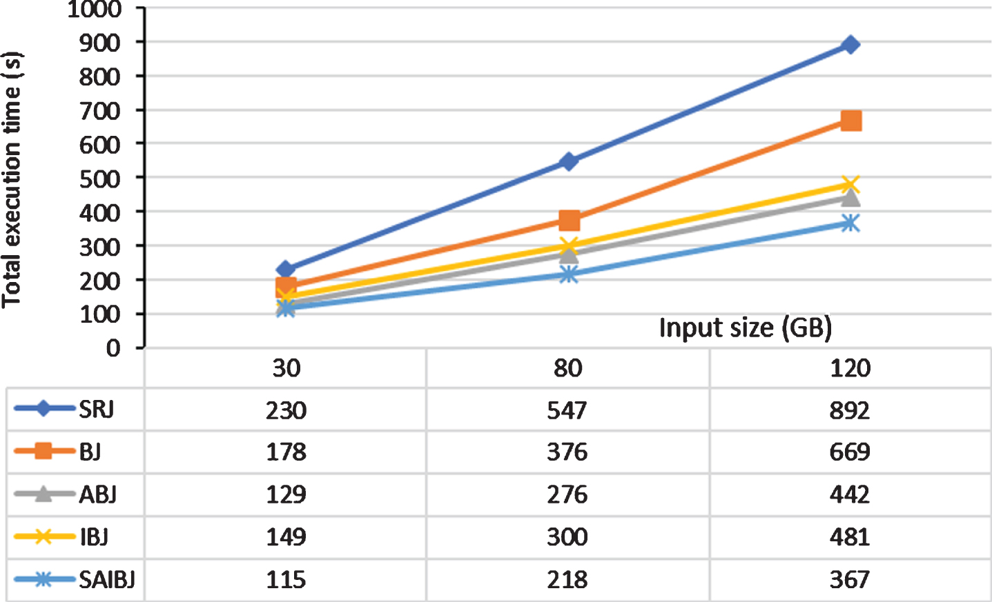
The total execution time of the join algorithms with varying input size (Set₁, Set₂, Set₃).

6 Conclusion and future work

The join operation is one of the most essential, costly, and frequently used operations for data analysis. Join processing using MapReduce is expensive and not easy to implement. In Section 2, we summarized the state-of-the-art studies that address this issue.

The implementation of the adaptive filter-based join algorithms was described in Section 3. We adapted the concept of filter creation and redundant records elimination within a single MapReduce job and without any prior modifications to the MapReduce architecture. Two strategies were presented in order to dynamically build and distribute the filters. Strategy₁ builds the global filter in a distributed manner. On the other hand, strategy₂ computes the global filter in a central manner. Theoretically, it has been proven that strategy₁ is well suited for small input sizes while strategy₂ is well suited for large input sizes. The cost analysis presented in Section 4 shows the introduced algorithms reduce the total I/O cost compared to the state-of-the-art filter-based joins, for all Bloom filter sizes less than a certain fraction (α) of the input split size.

The conducted experiments in Section 5 were divided into four tests. Test₁ and Test₂ examined the effect of varying the input size and join ratio, respectively. Test₃ evaluated the performance of the adaptive intersection Bloom join. Test₄ examined the effect of varying the Bloom filter size. The performance of the join algorithms was evaluated in terms of the total execution time and the total amount of I/O data. The experimental results show that the adaptive Bloom join, semi-adaptive intersection Bloom join and adaptive intersection Bloom join decrease the total execution time by averages of 30%, 25%, and 35%, respectively, compared to the state-of-the-art filter-based joins and reduce the total amount of I/O data by percentages of 18%, 25%, and 50%, respectively.

In future work, we plan to extend the introduced algorithms to handle data skew problems. The new approach could retrieve crucial statistical information of the input datasets using the local filters and the hash table of each input split to allow for load balancing Also, we plan to integrate our algorithms in current distributed engines such as Spark and Flink and investigate the potential of building a foundation of a query processing system that selects the most efficient join algorithm.

References

Marr

, Big Data: Using SMART Big Data, Analytics and Metrics to Make Better Decisions and Improve Performance 1st ed. UK: John Wiley & Sons. (2015).

Reinsel

, Gantz

and Rydning

, Data Age 2025: The Evolution of Data to Life-Critical. Sponsored by Seagate, International Data Corporation (IDC), (2017).

Dean

and Ghemawat

, MapReduce: Simplified Data Processing on Large Clusters, Communications of the ACM 51(1) (2008), 107–113.

Cooper

B.F.

, Ramakrishnan

, Srivastava

, Silberstein

, Bohannon

, Jacobsen

H.A.

, Puz

, Weaver

and Yerneni

, PNUTS: Yahoo!’s Hosted Data Serving Platform, Proceedings of the VLDB Endowment 1(2) (2008), 1277–1288.

Chaiken

, Jenkins

, Larson

P.Å.

, Ramsey

, Shakib

, Weaver

and Zhou

, SCOPE: Easy and Efficient Parallel Processing of Massive Data Sets, Proceedings of the VLDB Endowment 1(2) (2008), 1265–1276.

Zaharia

, Xin

R.S.

, Wendell

, Das

, Armbrust

, Dave

, Meng

, Rosen

, Venkataraman

, Franklin

M.J.

and Ghodsi

, Apache spark: A Unified Engine for Big Data Processing, Communications of the ACM 59(11) (2016), 56–65.

Sivarajah

, Kamal

M.M.

, Irani

and Weerakkody

, Critical analysis of Big Data challenges and analytical methods, Journal of Business Research 70 (2017), 263–286.

Lee

K.H.

, Lee

Y.J.

, Choi

, Chung

Y.D.

and Moon

, Parallel Data Processing with MapReduce: A Survey, ACM SIGMOD Record 40(4) (2012), 11–20.

Palla

, A Comparative Analysis of Join Algorithms using the Hadoop Map/Reduce Framework, Master of science thesis, School of Informatics, University of Edinburgh, (2009).

10.

Blanas

, Patel

J.M.

, Ercegovac

, Rao

, Shekita

E.J.

and Tian

, A Comparison of Join Algorithms for Log Processing in MapReduce, In Proceedings of the 2010 ACM SIGMOD International Conference on Management of data. ACM, (2010), 975–986.

11.

Lee

, Bae

H.C.

and Kim

H.J.

, Join Processing with Threshold-Based Filtering in MapReduce, The Journal of Supercomputing 69(2) (2014), 793–813.

12.

Lee

, Kim

and Kim

H.J.

, Exploiting Bloom Filters for Efficient Joins in MapReduce, International Information Institute (Tokyo) Information 16(8) (2013), 5869–5885.

13.

Lee

, Kim

and Kim

H.J.

, Join Processing using Bloom Filter in MapReduce, In Proceedings of the 2012 ACM Research in Applied Computation Symposium. ACM, (2012), 100–105.

14.

Phan

T.C.

, d’Orazio

and Rigaux

, A Theoretical and Experimental Comparison of Filter-Based Equijoins in MapReduce, Transactions on Large-Scale Data-and Knowledge-Centered Systems XXV 9620 (2016), 33–70.

15.

Phan

T.C.

, d’Orazio

and Rigaux

, Toward Intersection Filter-Based Optimization for Joins in MapReduce, In Proceedings of the 2nd International Workshop on Cloud. ACM, (2013), Article No. 2.

16.

Matono

, Ogawa

and Kojima

, Improvement of Join Algorithms for Low Selectivity Joins on MapReduce, In Australasian Database Conference. Springer, (2015), 117–128.

17.

Zhang

, Wu

and Li

, Optimizing Distributed Joins with Bloom Filters Using MapReduce, In Computer Applications for Graphics, Grid Computing, and Industrial Environment. Springer, (2012), 88–95.

18.

Gavagsaz

, Rezaee

and Javadi

H.H.S.

, Load Balancing in Join Algorithms for Skewed Data in MapReduce Systems, The Journal of Supercomputing 75(1) (2019), 228–254.

19.

Fier

, Augsten

, Bouros

, Leser

and Freytag

J.C.

, Set Similarity Joins on MapReduce: An Experimental Survey, Proceedings of the VLDB Endowment 11(10) (2018), 1110–1122.

20.

Afrati

F.N.

and Ullman

J.D.

, Optimizing Joins in a Map-Reduce Environment, In Proceedings of the 13th International Conference on Extending Database Technology. ACM, (2010), 99–110.

21.

Bruno

, Kwon

and Wu

M.C.

, Advanced Join Strategies for Large-Scale Distributed Computation, Proceedings of the VLDB Endowment 7(13) (2014), 1484–1495.

22.

Al-Badarneh

A.F.

and Rababa

S.A.

, An Analysis of Two-Way Equi-Join Algorithms Under MapReduce, Journal of King Saud University –Computer and Information Sciences (2020), https://doi.org/10.1016/j.jksuci.2020.05.004.

23.

Potluri

, Bhattu

S.N.

, Kumar

N.N.

and Subramanyam

R.B.V.

, Design Strategies for Handling Data Skew in MapReduce Framework, In Proceedings of International Conference on Inventive Computation Technologies. Springer, (2020), 240–247.

24.

Atta

, Viglas

S.D.

and Niazi

, SAND Join—A Skew Handling Join Algorithm for Google’s MapReduce Framework, In Proceedings of the 14th International Multitopic Conference (INMIC). IEEE, (2011), 170–175.

25.

Afrati

F.N.

, Stasinopoulos

, Ullman

J.D.

and Vassilakopoulos

, SharesSkew: An Algorithm to Handle Skew for Joins in MapReduce, Information Systems 77 (2018), 129–150.

26.

Myung

, Shim

, Yeon

and Lee

S.G.

, Handling Data Skew in Join Algorithms Using MapReduce, Expert Systems with Applications 51 (2016), 286–299.

27.

Hassan

M.A.H.

and Bamha

, Towards Scalability and Data Skew Handling in GroupBy-Joins using MapReduce Model, Procedia Computer Science 51 (2015), 70–79.

28.

Jiang

, Tung

A.K.

and Chen

, MAP-JOIN-REDUCE: Toward Scalable and Efficient Data Analysis on Large Clusters, IEEE Transactions on knowledge and Data Engineering 23(9) (2011), 1299–1311.

29.

Yang

H.C.

, Dasdan

, Hsiao

R.L.

and Parker

D.S.

, MAP-REDUCE-MERGE: Simplified Relational Data Processing on Large Clusters. In Proceedings of the 2007 ACM SIG-MOD International Conference on Management of Data. ACM, (2007), 1029–1040.

30.

Pigul

, Comparative Study Parallel Join Algorithms for MapReduce Environment, Proceedings of the Institute for System Programming 23 (2012), 285–306.

31.

Atta

, Implementation and Analysis of Join Algorithms to Handle Skew for the Hadoop Map/Reduce Framework, Master of science thesis, School of Informatics, University of Edinburgh, (2010).

32.

White

, Hadoop: The Definitive Guide. 4th ed. USA: O’Reilly Media, Inc. (2015).

33.

Sundarrajan

and Shivalingamurthy

, Method and system for optimizing reduce-side join operation in a map-reduce framework, U.S. Patent No. 10,185,743. (2019).

34.

Mackert

L.F.

and Lohman

G.M.

, R* Optimizer Validation and Performance Evaluation for Distributed Queries, In Proceedings of the 12th International Conference on Very Large Data Bases. ACM, (1986), 219–229.

35.

Bloom

B.H.

, Space/Time Trade-offs in Hash Coding with Allowable Errors, Communications of the ACM 13(7) (1970), 422–426.

36.

Lam

, Hadoop in Action, 1st ed. USA: Manning Publications Co. (2010).

37.

Zhang

, Wu

and Li

, Efficient Processing Distributed Joins with Bloom Filter using MapReduce, International Journal of Grid Distributed Computing 6(3) (2013), 43–58.

38.

Koutris

, Bloom Filters in Distributed Query Execution. University of Washington, USA. [Online] Available at: https://courses.cs.washington.edu/courses/cse544/11wi/projects/koutris.pdf, (2011), [Accessed on 7 January 2019].

39.

Tran

, Phan

, Laurent

and D’Orazio.

, Improving Hamming distance-based fuzzy join in MapReduce using Bloom Filters, In 2018 IEEE International Conference on Fuzzy Systems (FUZZ-IEEE), IEEE, (2018), 1–7.

40.

Tran

, Phan

, Laurent

and D’Orazio.

, Optimization for Large-Scale Fuzzy Joins Using Fuzzy Filters in MapReduce, In 2020 IEEE International Conference on Fuzzy Systems (FUZZ-IEEE). IEEE, (2020), 1–8.

41.

Broder

and Mitzenmacher

, Network Applications of Bloom Filters: A Survey, Internet Mathematics 1(4) (2004), 485–509.

42.

Nykiel

, Potamias

, Mishra

, Kollios

and Koudas

, MRShare: Sharing Across Multiple Queries in MapReduce, Proceedings of the VLDB Endowment 3(1-2) (2010), 494–505.

43.

Ahmad

, PUMA Benchmarks and Dataset Downloads, [Online] Available at: https://engineering.purdue.edu/ puma/datasets.htm., (2012), [Accessed on 14 November 2019].

Optimizations for filter-based join algorithms in MapReduce

Abstract

Keywords

1 Introduction

2 Related work

3 Implementation of adaptive filter-based join algorithms

3.1 Algorithm1: Adaptive Bloom Join

Table 1 Abbreviations for representing the join algorithms Abbreviation Algorithm SRJ Standard Repartition Join BJ Bloom Join IBJ Intersection Bloom Join ABJ Adaptive Bloom Join SAIBJ Semi-Adaptive Intersection Bloom Join AIBJ Adaptive Interaction Bloom Join

Table 3 Cluster characteristics Node Role Memory CPU Hard Disk Node 0 NameNode/ResourceManager 252GB 32vCPU – Node 1 DataNode/NodeManager 63GB 32vCPU 17TB Node 2 DataNode/NodeManager 63GB 32vCPU 17TB Node 3 DataNode/NodeManager 63GB 32vCPU 28TB

Table 4 Test1 input datasets Input Dataset 1 Dataset 2 Set 1 size 15GB 15GB # of records 37,571,850 37,428,177 Set 2 size 40 40 # of records 102,322,416 101,983,585 Set 3 size 60GB 60GB # of records 161,030,087 161,029,465

Table 6 Test3 input datasets Inputs Size Number of records Dataset 1 2GB 5,367,350 Dataset 2 2GB 5,367,783 Total 4GB 10,735,133

Table 7 Number of intermediate records Approach Set1 (30GB) Set2 (80GB) Set3 (120GB) SRJ 74,956,106 204,187,414 321,998,184 BJ and ABJ 37,424,639 101,967,321 161,003,151 IBJ and SAIBJ 80,643 204,187 331,580

References

3.1 Algorithm₁: Adaptive Bloom Join

Table 1
Abbreviations for representing the join algorithms

Abbreviation Algorithm

SRJ Standard Repartition Join

BJ Bloom Join

IBJ Intersection Bloom Join

ABJ Adaptive Bloom Join

SAIBJ Semi-Adaptive Intersection Bloom Join

AIBJ Adaptive Interaction Bloom Join

Table 3
Cluster characteristics

Node Role Memory CPU Hard Disk

Node ₀ NameNode/ResourceManager 252GB 32vCPU –

Node ₁ DataNode/NodeManager 63GB 32vCPU 17TB

Node ₂ DataNode/NodeManager 63GB 32vCPU 17TB

Node ₃ DataNode/NodeManager 63GB 32vCPU 28TB

Table 4
Test₁ input datasets

Input Dataset ₁ Dataset ₂

Set ₁ size 15GB 15GB

# of records 37,571,850 37,428,177

Set ₂ size 40 40

# of records 102,322,416 101,983,585

Set ₃ size 60GB 60GB

# of records 161,030,087 161,029,465

Table 6
Test₃ input datasets

Inputs Size Number of records

Dataset ₁ 2GB 5,367,350

Dataset ₂ 2GB 5,367,783

Total 4GB 10,735,133

Table 7
Number of intermediate records

Approach Set₁ (30GB) Set₂ (80GB) Set₃ (120GB)

SRJ 74,956,106 204,187,414 321,998,184

BJ and ABJ 37,424,639 101,967,321 161,003,151

IBJ and SAIBJ 80,643 204,187 331,580