Spatio-temporal K-NN prediction of traffic state based on statistical features in neighbouring roads

Abstract

Traffic congestion on a road results in a ripple effect to other neighbouring roads. Previous research revealed existence of spatial correlation on neighbouring roads. Similar traffic patterns with regards to day and time can be seen amongst roads in a neighbouring area. Presently, nonlinear models of neural network are applied on historical data to predict traffic congestion. Even though neural network has successfully modelled complex relationships, more time is needed to train the network. A non-parametric approach, the k-nearest neighbour (K-NN) is another method for forecasting traffic condition which can capture the nonlinear characteristics of traffic flow. An earlier study has been done to predict traffic flow using K-NN based on connected roads (both downstream and upstream). However, impact of road congestion is not only to connected roads, but also to roads surrounding it. Surrounding roads that are impacted by road congestion are those having ‘high relationship’ with neighbouring roads. Thus, this study aims to predict traffic state using K-NN by determining high relationship roads within neighbouring roads. We determine the highest relationship neighbouring roads by clustering the surrounding roads by combining grey level co-occurrence matrix (GLCM) with k-means. Our experiments showed that prediction of traffic state using K-NN based on high relationship roads using both GLCM and k-means produced better accuracy than using k-means only.

Keywords

Classification algorithm clustering algorithm machine learning algorithm nearest neighbour search intelligent transportation system

1 Introduction

Growing population as well as surge in the number of vehicles in urban areas have led to worsening of traffic congestion, causing stress [1] and economic losses, as well as increase in pollution that hampers the environment [2]. Thus, if drivers are provided with traffic information, it would help them with their driving plans, including changing their driving habits as well as choosing driving paths [3]. Furthermore, if traffic information is available, it could result in a chain of movement in traffic state both in downstream and upstream of road segments in the same area.

Traffic jam or congestion is regarded as a situation in which the number of road users surpasses the capacity of the road. Some inherent characteristics of road congestion include long queue, long travelling time, and slow speed of vehicles on the road. Thus, it is important to develop effective algorithm or models to identify congested roads, to analyse congestion distribution in the network and to determine relationship between increasing traffic flow and occurrence of congestion. Some of the research works have employed neural network to predict traffic flow, by considering all day’s data of traffic flow of neighbouring road [4] as well as predicting the traffic flow on road intersections using data on all day’s data [5].

Other studies have shown that adjacent roads demonstrated a similar traffic pattern on the same time interval and day [6, 7]. Studying traffic patterns in adjacent roads can lead to discovery of relationships amongst roads in a neighbouring area. This information is important in studies of traffic state as the results can be used to assist drivers in avoiding congested roads and nearby roads which are affected by the congestion. Moreover, identifying relationships amongst roads in a neighbouring area can produce higher accuracy of traffic state prediction. Based on Fig. 1, we can expect that traffic flow on road I, will also impact the traffic flow on surrounding roads like road II, road III and road IV. In other words, traffic flow on road III would be impacted by traffic flows of neighbouring roads.

Fig. 1

Illustrations for high relationship roads impacting traffic flow.

There exists correlation between connected road segments in either downstream, upstream or both [4, 8]. Other research studies also determined the existence of congestion correlation for two road segments [9], between two road segments I and II at a given distance d. This means that if there is congestion in road I at time t and at time t + T, then it results in congestion even in road II. In a different research study, data extracted from sensors was used to determine the relationships amongst road segments using correlation method [10, 11].

Traffic condition is regarded to be nonlinear, uncertain and complex. Thus, it becomes difficult to accurately predict the traffic condition by making use of prediction methods based on regular mathematics models [12]. Previously, the neural network was used by considering the historical data to develop complex relationship models pertaining to traffic flow. However, training the network takes a long time [13]. Thus, the K-nearest neighbour (K-NN), a non-parametric method is a better approach to forecast short-term traffic condition. Various studies have used K-NN to predict short-term traffic flow [13, 14], using three-layer K-NN [15], using with or without weight [12] and using similar data [16].

The research using K-NN to predict traffic state that is closest with our work is [8, 17]. They used connected roads both upstream and downstream [8] and surrounding roads as spatial relationship [17]. However, impact of road congestion is not only to connected and surrounding roads. Road congestion is also impacted by roads having ‘relationship’ with the congested road. Other research that related with our study is [18]. They reduce spatial temporal feature using tensor algebra. Another study by [19, 20] use k-means cluster of similarity traffic in neighbouring roads.

In this study, we proposed spatio-temporal K-NN model to predict traffic state. The acquired spatial information is based on the similarity of traffic flow features among roads. The features of traffic flow are extracted using grey level co-occurrence matrix (GLCM). The extracted features are then clustered using k-means to obtain roads that are related to each other, or in other words having ‘relationship’. Roads with high relationship are then used as spatial relationship for prediction using K-NN. Our study shows that combining GLCM with k-means clustering produced better prediction of traffic state in comparison with prediction based on k-means without GLCM.

The rest of the paper is structured as follows. Section II introduces our method to construct a nonparametric k-nearest model. Section III discusses results of our experiment. Lastly, we present our conclusion of our work.

2 Methodology

2.1 Congestion index and congestion determination

In order to determine the level of road congestion, various definitions and variables of traffic congestion were formed. Traffic congestion rank was defined by Rothenberg [21] as the condition in which the number of vehicles on the road surpasses the carrying capacity of the standard road service level. Another study used congestion index by considering the saturation degree, travelling speed and a combination of both [22]. A different study accounted for the speed performance index by segmenting congestion level as four, three or two as needed [23]. In this study, the congestion index for a given time interval was determined to calculate similarity between roads to obtain the congestion level.

Congestion index was calculated based on the travelling speed [22], with some adjustments. Instead of hourly calculation, congestion index was calculated at every 20 minutes using the formula given in (1). For example, for road 158324, congestion index was calculated at every 20 minutes from 05:00 to 09:20 AM as presented in Table 1. For neighbouring roads, congestion index was calculated every day from February 2014 until September 2014.

$CI = \frac{NDT - {Vavg}_{interval time}}{NDT - {Vmin}_{interval time}} \times \frac{{Volume}_{interval time}}{{Volume}_{day}} \times 100$ (1)

Table 1

Details of data from sensor 173011

Time (Start End)	Coordinates (Start End)	Normal Driving Time
10/1/2014 1:45:00 AM	Latitude: 56.215 Longitude: 10.139 City: Aarhus Street: SÃ¸ftenvej Postal Code: 8382	NDT: 51km/h Distance: 2061 (m) Duration: 100s Type: STREET
11/13/2014 10:40:00 AM	Latitude: 56.213 Longitude: 10.116 City: Hinnerup Street: Rhusvej Postal Code: 8200

NDT: normal driving time in kilometre per hour or speed limit, as shown in Table 1.

Vavg_{interval time}: average speed in interval hours

Vmin_{interval time}: minimum speed in interval hours

Volume_{interval time}: number of vehicles in interval hours

Volume_day: number of vehicles in a day

As observed in Fig. 2, the road congestion occurred between 06:10 AM until 08:10 AM. From Table 2 show that, the congestion index was found between three (3.03) to five (5.41). In Denmark, the average speed of normal traffic in town is 50km/hour [24]. Based on this information, we defined traffic congestion as the situation when average speed is below 50km/h. As we can observed from Table 2, when the average speed is 50km/hour, the congestion index value is around 3. Thus, for this study, we consider that a road is congested when the congestion index is above or equals 3.

Fig. 2

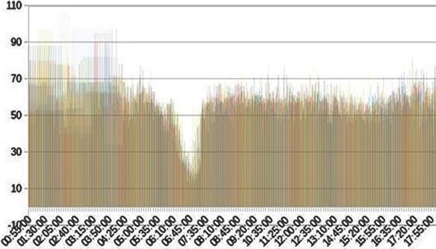
The average speed on road 158324 every five minutes.

Table 2

Congestion on Road 158324 from 06.00-08.20 AM

Time	Congestion Index	Average				Volume
5:40-6:00	2.73	63	62	57	57	4	6	14	17
6:00-6:20	3.03	57	55	50	50	12	12	15	13
6:20-6:40	3.83	41	41	47	45	16	20	11	11
6:40-7:00	4.52	45	47	39	28	12	12	20	23
7:00-7:20	4.25	23	25	25	14	24	21	15	17
7:20-7:40	5.41	13	13	14	15	22	20	17	15
7:40-8:00	3.98	21	23	26	48	18	30	22	16
8:00-8:20	3.71	53	56	56	57	11	20	18	13
8:20-8:40	2.6	58	57	52	59	13	8	14	10
8:40-9:00	2.69	68	58	51	52	7	10	12	9
9:00-9:20	2.81	57	60	61	58	5	5	9	12

2.2 Spatial relationship with grey level co-occurrence matrix

In this study, we use grey level co-occurrence matrix (GLCM) fusion with k-means to find the relationship between roads. GLCM refers to a method for describing texture by studying the spatial correlation characteristics of grayscale. Since traffic flow pattern is formed by the repeated occurrence of the congestion distribution in the spatial position, there will be a certain traffic state relationship between two matrix values at a certain distance in the traffic state space. This is the spatial correlation characteristics of traffic state. Traffic congestion has same pattern in interval time and interval day as shown in Table 3. Based on this pattern, we set our GLCM matrix with a horizontal offset of 2 to the right and vertical offset of 2 downwards. By referring to Fig. 2, 0 indicates clear state and 1 indicates congestion state.

Table 3
Traffic congestion pattern in time and day on road 158324, road 158386, and road 158536

Contrast is a measure of intensity between a matrix value and its neighbour over the whole matrix [25 –27]. Contrast is calculated using equation (2) and correlation of a matrix value to its neighbour is given by the equation (3). Homogeneity is a value that measures the closeness of the distribution of elements in the GLCM to the GLCM diagonal. It is given by equation (5). Energy is the sum of squared elements in normalized GLCM. It is given by equation (4). $Contrast = \sum_{i, j} {| i - j |}^{2} p {(i, j)}^{2}$ (2) $Correlation = \frac{(i - μ i) (j - μ j) p (i, j)}{σ_{i} σ_{j}}$ (3) $Energy = \sum_{i, j} p {(i, j)}^{2}$ (4) $Homogeneity = \sum_{i, j} \frac{(j - μ j) p (i, j)}{1 + | i - j |}$ (5)

K-means is a data grouping algorithm that will divide data into several k groups. It is a very famous algorithm because of its simplicity [28]. This algorithm tries to divide the data into k groups. Where data from a group will have the same character between each of its members. On the other hand, the data in a group will have different character from other group members. This algorithm tries to find variations that are very minimal between the same groups and will look for variations that are maximum with other groups [29]. The algorithm used is as follows:

Specify k=six (6). This value is obtained by observing the elbow curves in Fig. 3. From Fig. 3, it can be seen that all roads have similar pattern. The elbow points are around 6.

Randomly select k distinct data points as initial cluster means.

Then, compute the Euclidean distance between each mean cluster and all other points.

Assign each point to the cluster having the closest mean.

Move the centroid. Recalculate the cluster centroid (means) for each of the k clusters by computing the new mean value of all the data points in the cluster.

Do steps 3 to 5 repeatedly, until the centroids stop moving. or they reach the maximum number of repetitions.

Fig. 3

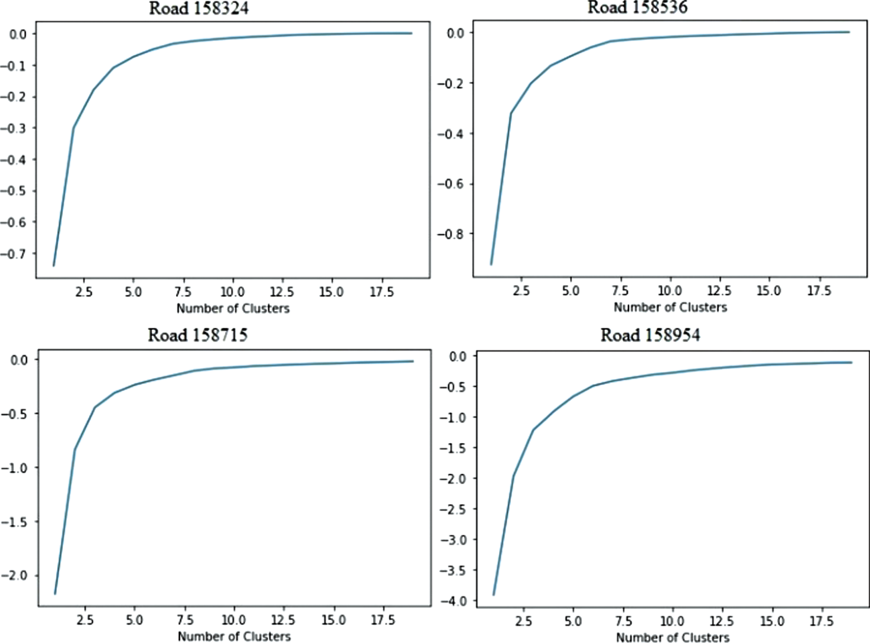
Elbow curves for road 158536, road 178600, road 210173 and road 195817.

The total within the sum of squares or the total within-cluster variation is defined as: $\sum_{k = 1}^{4} W (C_{k}) = \sum_{k = 1}^{4} \sum_{x_{i} \in C_{k}} {(x_{i} - μ_{k})}^{2}$ (6)

Where:

x_i is data point member of the cluster C_k

μ_k is the mean value of the points defined to the cluster C_k.

2.3 Spatio-temporal K-NN model

The k-Nearest Neighbour (K-NN) is a straightforward machine-learning non-parametric technique, that is, without model and without any parameter. The primary principle of this technique is that if k number of most similar samples in the feature space are of one group in the dataset, then the sample belongs to that group. The concept of K-NN is given in Fig. 4. Assume that the elements in the data set are represented by triangles and squares as shown in the figure. Supposedly, we need to find out the category to which the brown circle belongs to. It depends on the value of k. If k=3, then the 3 nearest neighbours to the brown circle are 2 squares and one triangle. Then, this brown circle is regarded as belonging to the square category on the basis of the statistics. If k=6, then the six nearest neighbours to the brown circle are 4 triangles and 2 squares. Thus, this brown circle is regarded as belonging to the triangle category as can be seen from the statistics.

Fig. 4

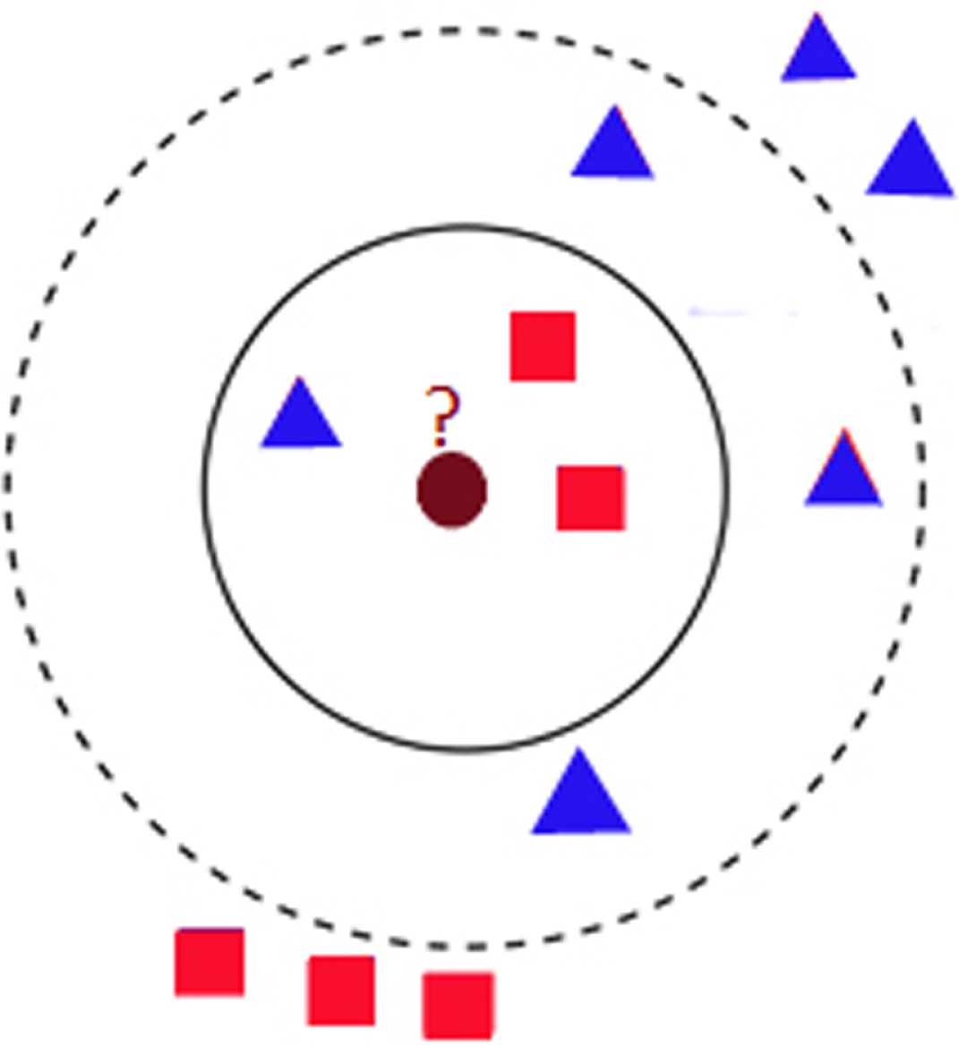
Example of k-NN concept.

In this study, the K-NN technique is applied to estimate short-term traffic condition. The technique searches for the nearest matching neighbours between previous data according to similarity of time and data value based on distance between historical data and current data. There is no need to specify in advance the mathematical model or the parameters. Detailed explanation for the K-NN technique is explained in [8, 12]. Distance, state vector, number of nearest neighbours and prediction algorithm are included in the K-NN technique. The distance and prediction algorithms are explained in more depth as follow:

The distance is required for comparing the value among the test data and sample data. Data having the nearest distance between historical data and sample data are then chosen to be used in the K-NN model. This data is then used in the prediction algorithm. We consider Euclidean distance as distance in this study. See Equation (7).

Traffic congestion index on a road changes according to day of the week and duration of time. So different days and different time intervals affect the future of traffic conditions. For the same time (time and day) in both historical and forecast data, distance between time in forecasting and state vector should be as small as possible. $d_{i} = \sqrt{\sum_{j} {(T_{j} - t_{ji})}^{2} + {(V_{j} - v_{ji})}^{2}}$ (7)

where

d_i=distance of group i between forecast data and historical data;

Vj=congestion index value of vector j in forecast data;

v_ji=congestion index value of state vector j in historical data i.

Typically the K Number chosen is the square root of the N training data [30]. In this study, the neighbouring results are obtained from clustering (GLCM with k-means). The K-NN estimations are based on a voting process, statistically.

For our study, we proposed the spatio-temporal K-NN algorithm, as shown in Fig. 5. For state vector, we consider historical data (t) of the traffic congestion index on the destination road and neighbouring roads of the same cluster (GLCM with KNN). K-NN model is then used to predict traffic condition on destination road (t+1).

Fig. 5

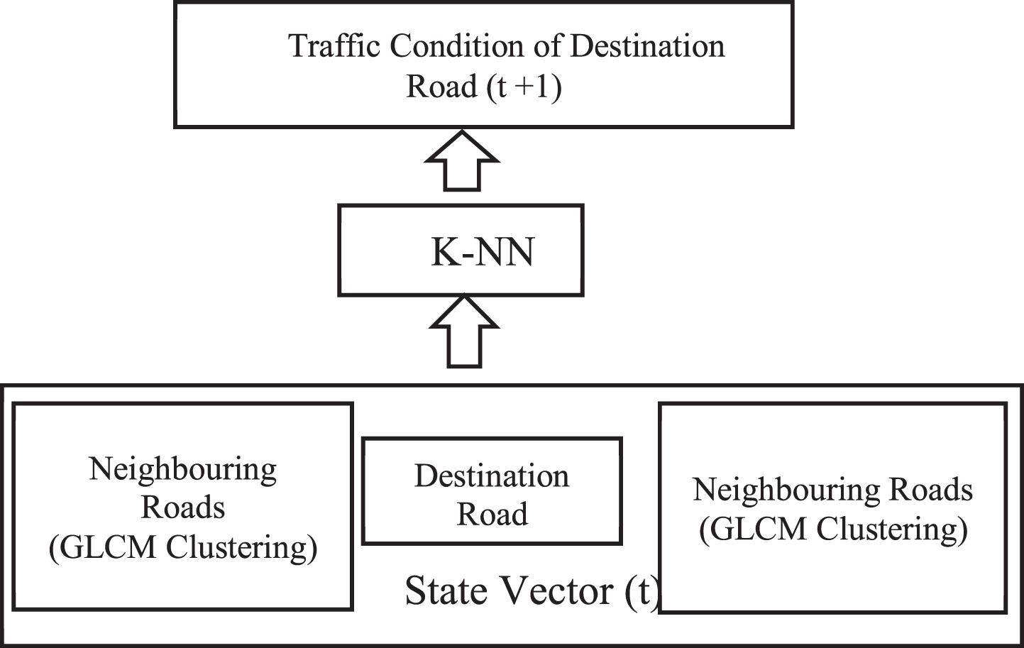
Spatio temporal K-NN model for predicting traffic state.

2.4 Similarity traffic condition

Some studies discovered that there is a difference in traffic flow pattern on weekends and on weekdays [6, 31]. We considered the road 158324 for studying traffic flow pattern and found that there exists a similar pattern of the traffic flow on weekdays. The weekdays’ data is traffic data from Monday to Thursday while the weekends data is traffic data from Friday to Sunday as seen in Fig. 6.

Fig. 6

Traffic pattern on road 158324, (a) pattern on weekdays, (b) pattern on weekends.

3 Result and discussion

3.1 Dataset

In this study, we used the dataset obtained from the IoT traffic sensors located in Aarhus, Denmark [32 –34]. The approximate number of sensors at this place is 449 as displayed in Fig. 7.

Fig. 7

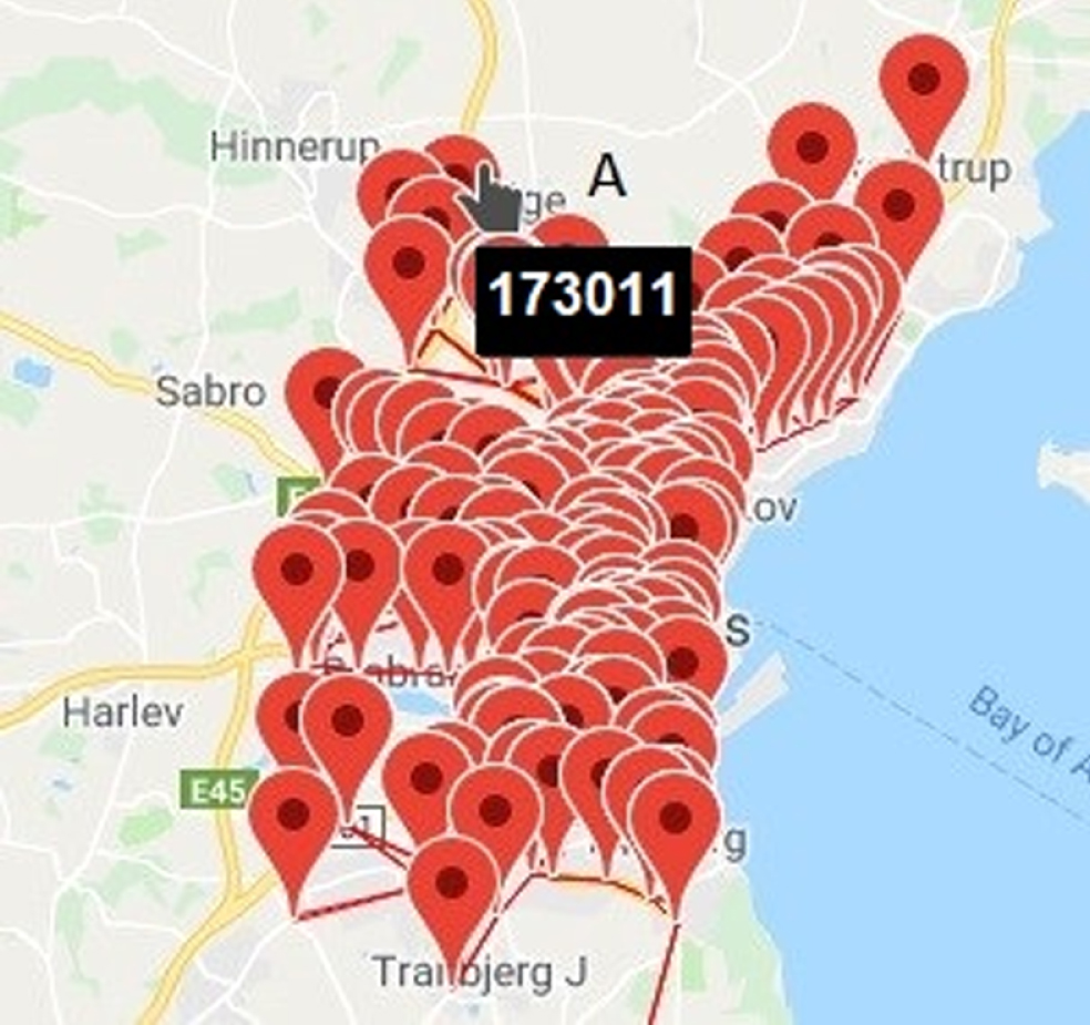
Map of location of 449 IoT traffic sensors in the city of Aarhus, Denmark.

For instance, the sensor at location A is identified by 173011. This sensor is placed at SÃ¸ftenvej Street, Aarhus city and at rhusvej Street, Hinnerup city, Denmark. The distance between both the sensors is 2061 metres. We conducted the experiment using vehicle count, average speed and time to calculate the congestion index. Example of data taken from sensor 173011 are presented in Table 4.

Table 4

Example of traffic data taken from sensor 173011

Average Time	Average Speed	Time Median	Time Time	Vehicle Count
226	51	226	15:40:00	1
211	55	211	2014-02-13	2
211	55	211	15:45:00	2
			2014-02-13
			15:50:00
			2014-02-13

3.2 Results

In this paper, we present results of traffic flow prediction at 10 different neighbouring areas which cover the road 158536, road 178600, road 210173, road 195817, road 185131, road 178767, road 195286, road 188225, road 201855, and road 206316 as seen in Fig. 8. We define neighbouring roads as roads within the radius of four (4) kilometres or less from a target location.

Fig. 8

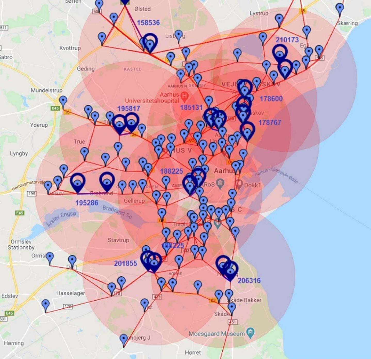
Map of 10 neighbouring areas in the city of Aarhus, Denmark considered in experiment.

We compare K-NN results obtained from k-means clustering against K-NN result obtained from GLCM-k-means clustering method. Since we are interested to predict traffic flow for the weekdays, we compute the similarity of the congestion index on weekdays starting from 15 Feb 2014 to 31 May 2014. Detailed explanations are provided in section 2.1. We split 20 percent of our dataset for testing the proposed K-NN model.

We observed that clustering using k-means obtained higher number of roads if compared with clustering using GLCM and kmeans. The combination of GLCM with kmeans filtered more roads which have relationship with target road. We also compared our results with roads obtained by Pearson correlation. Using this method, we filter only roads that have correlation value above 0.5. Therefore, we only visualized location of the three roads with correlation value above 0.5 namely road 158536, road 195286 and road 201855.

The results of clustering on location 158536 are shown in Fig. 9. The combination of GLCM with k-means filtered more roads that have relationship with road 158536. When using Pearson correlation, we obtained 18 roads which is three roads more than using k-means method.

Fig. 9

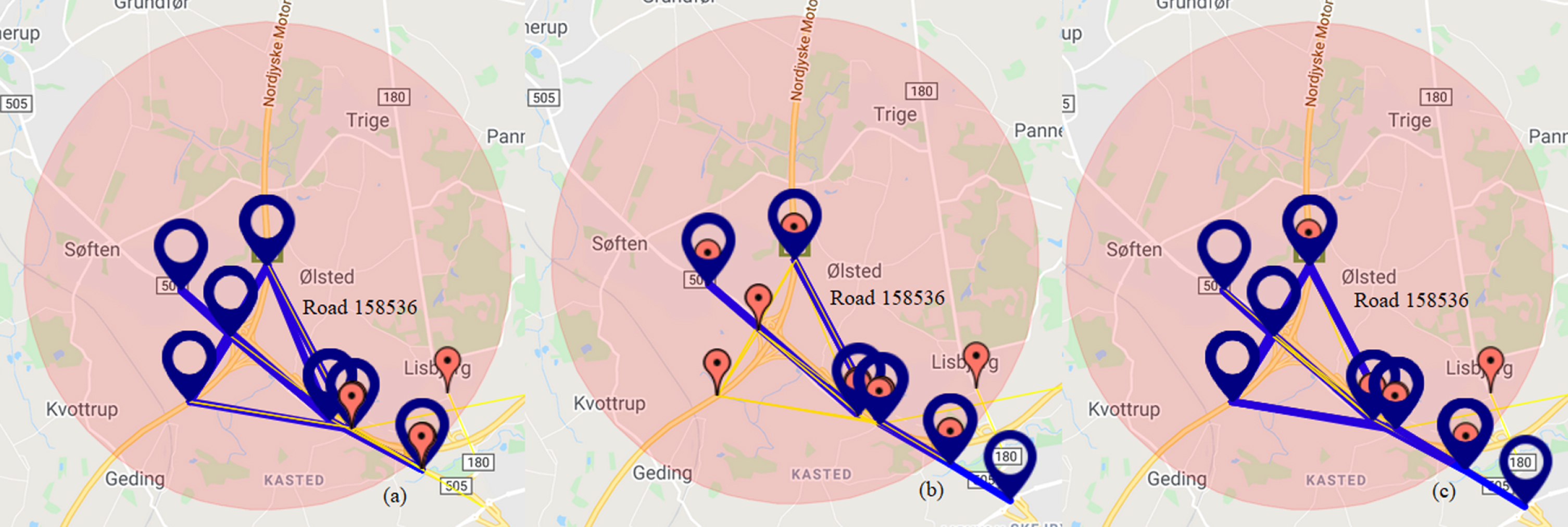
Traffic pattern on road 158536, (a) clustering with k-means, (b) clustering with GLCM and k-means, (c) high Pearson correlation value.

Figure 10 shows the results of clustering for location 195286. It can be seen from Fig. 10 that when using k-means we obtained more roads than when using GLCM. Clustering using combination of GLCM and k-means filtered more roads that have relationship with road 195286. When using Pearson correlation, we obtained three roads that have correlation value above 0.5 with road 195286. However, all methods obtained roads with distance outside 3.5km from road 195286.

Fig. 10

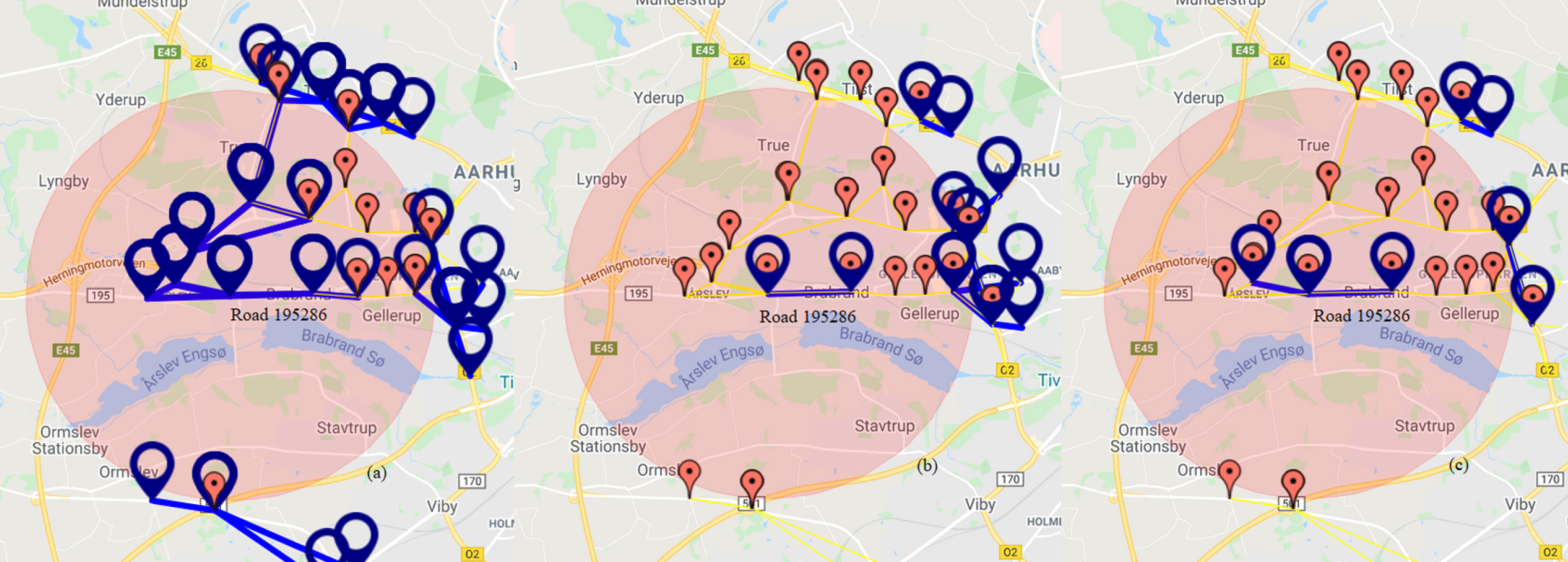
Traffic pattern on road 195286, (a) clustering with k-means, (b) clustering with GLCM and k-means, (c) high Pearson correlation value.

Figure 11 shows the results of clustering for location 201855. From Fig. 11, we observed that clustering using k-means obtained more roads when compared to clustering using GLCM. Clustering results of GLCM with k-means filtered more roads which have relationship with road 201855. Using Pearson correlation, we obtained one road that has correlation value above 0.5. All methods obtained roads outside 3.5km from road 201855, except when using Pearson correlation. However, the prediction accuracy (classification and regression) at location 201855 using clustering method is better when compared with Pearson correlation value.

Fig. 11

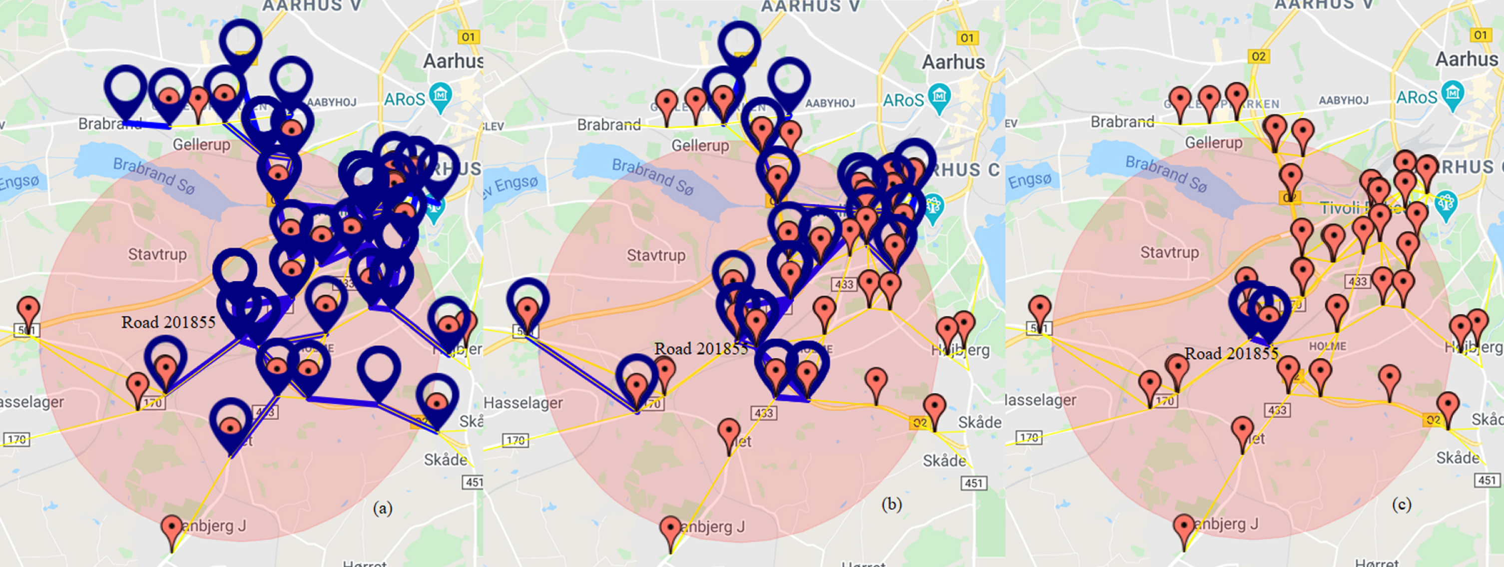
Traffic pattern on road 201855, (a) clustering with k-means, (b) clustering with GLCM and k-means, (c) high Pearson correlation value.

The neighbouring roads obtained by clustering method are then used for prediction of traffic state using K-NN. The prediction results of traffic state at location 158536 are presented in Table 5. The summary of traffic state predictions and prediction of average speed (regression) for all location are presented in Table 6.

Table 5

The result of prediction of road 158536, prediction of traffic state (classification) and prediction of average speed (regression)

K-Means (Accuracy)				GLCM K-Means (Accuracy)				Correlation (Pearson) (Accuracy)
Road	KNN Classification	KNN Regression	Linear Regression	Road	KNN Classification	KNN Regression	Linear Regression	Road	KNN Classification	KNN Regression	Linear Regression
158536	0.95	0.92	0.94	158536	0.95	0.92	0.94	158536	0.94	0.92	0.94
158475	0.95	0.88	0.91	173225	0.91	0.98	0.98	158475	0.91	0.88	0.91
172329	0.89	0.88	0.91	158386	0.96	0.90	0.92	173225	0.95	0.98	0.98
173225	0.92	0.98	0.98	158415	0.95	0.91	0.94	158355	0.94	0.87	0.89
158355	0.92	0.87	0.89	172602	0.92	0.95	0.97	171572	0.95	0.91	0.97
171572	0.85	0.91	0.97	158983	0.95	0.88	0.92	158324	0.95	0.90	0.93
158324	0.94	0.90	0.93					158386	0.92	0.90	0.92
158386	0.96	0.90	0.92					158446	0.93	0.89	0.91
158446	0.97	0.89	0.91					158595	0.96	0.91	0.93
158595	0.94	0.91	0.93					158895	0.84	0.90	0.92
158415	0.94	0.91	0.94					173118	0.92	0.96	0.98
158505	0.91	0.81	0.88					158565	0.85	0.89	0.93
173011	0.88	0.79	0.96					158624	0.97	0.89	0.93
158895	0.81	0.90	0.92					171969	0.94	0.89	0.93
173118	0.84	0.96	0.98					158715	0.81	0.90	0.92
								158744	0.95	0.91	0.93
								172602	0.94	0.95	0.97
								158983	0.94	0.88	0.92
Average	0.912	0.895	0.932	Average	0.940	0.922	0.947	Average	0.924	0.908	0.934

Table 6

The results of prediction for all location, prediction of traffic state (classification) and prediction of average speed (regression)

K-Means				GLCM K-Means			Correlation (Pearson)
Neighboring Area	Roads	KNN Classification	KNN Regression	Linear Regression	Roads	KNN Classification	KNN Regression	Linear Regression	Roads	KNN Classification	KNN Regression	Linear Regression
158536	15	0.911	0.895	0.932	7	0.944	0.922	0.947	18	0.923	0.908	0.934
195286	32	0.837	0.883	0.935	7	0.925	0.894	0.926	4	0.890	0.906	0.933
201855	55	0.864	0.832	0.943	24	0.915	0.816	0.942	2	0.907	0.694	0.940
178600	84	0.862	0.857	0.929	21	0.909	0.873	0.934
210173	32	0.807	0.851	0.932	14	0.851	0.843	0.944
195817	53	0.868	0.860	0.929	23	0.903	0.847	0.931
185131	94	0.882	0.861	0.924	71	0.916	0.873	0.930
178767	86	0.877	0.842	0.926	57	0.918	0.870	0.931	‘
188225	120	0.865	0.849	0.926	83	0.916	0.868	0.930
206316	53	0.868	0.814	0.938	35	0.872	0.821	0.951

3.3 Discussion

The results of experiment for all locations show that clustering using combination of GLCM and k-means produce fewer neighbouring roads than clustering using k-means. See Fig. 12. From Fig. 12, it can be seen that the Pearson correlation failed to obtain 7 high correlation roads out of 10. This is because traffic flow is nonlinear. Thus, pattern recognition is needed to obtain the relationship between roads.

Fig. 12

Number of high relationship roads among neighbouring roads obtained by different clustering method.

The average accuracy of prediction for traffic state (classification) of all roads using K-NN show that GLCM and k-means method performed the best when compared with k-means and Pearson correlation. This is shown in Fig. 13.

Fig. 13

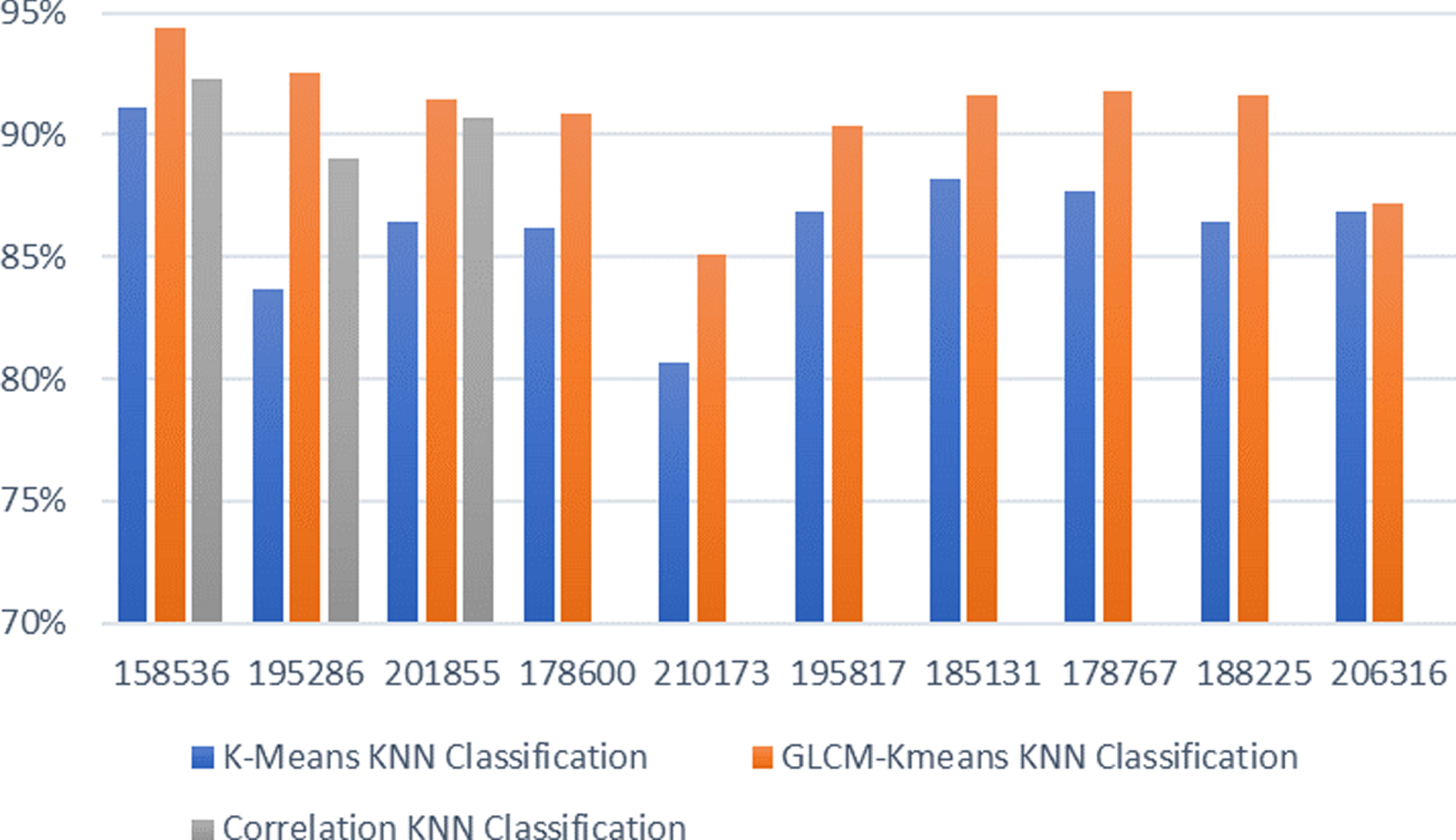
Comparison of traffic state prediction accuracy using the 3 methods for all locations.

To evaluate our findings, we calculate the prediction of average speed (regression). The results show that our proposed GLCM with k-means has better performance in predicting average speed using linear regression or KNN regression. This is shown in Fig. 14 and Fig. 15.

Fig. 14

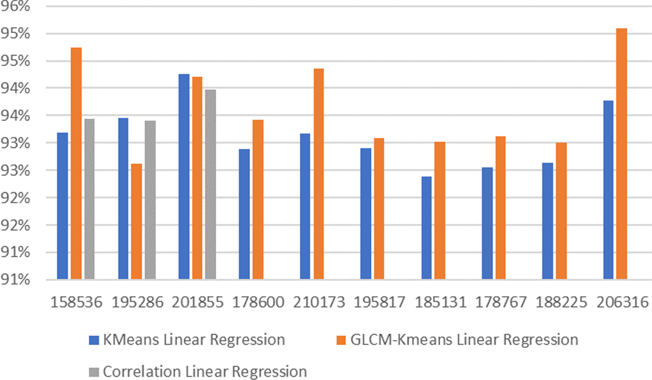
Comparison of average speed prediction accuracy using linear regression for all locations.

Fig. 15

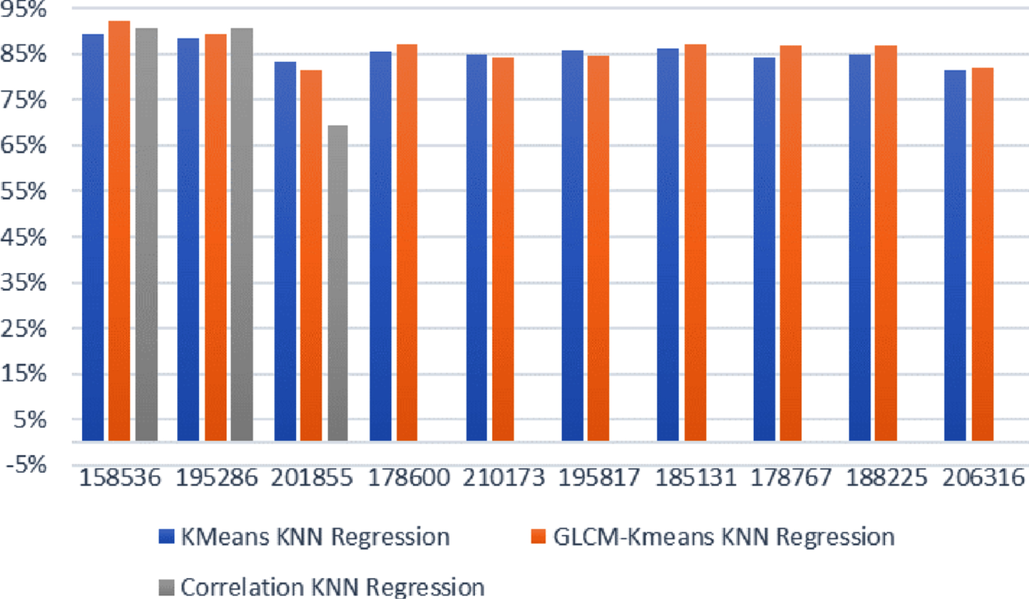
Comparison of the average speed prediction accuracy using knn regression for all locations.

Furthermore, the experimental results show that the high relationship roads obtained from GLCM with k-means improve prediction results for both traffic state (classification) and average speed (regression).

4 Conclusion

The main aim of our experiments in this study is to predict traffic state using K-NN based on highest relationship neighbouring roads. Highest relationship road is identified by obtaining the pattern of traffic congestion during day and time at a neighbouring area. We used the grey level co-occurrence matrix (GLCM) to extract the pattern of traffic congestion. GLCM is a method that has been widely used for pattern recognition. By combining GLCM with k-means, it improves the results in obtaining high relationship roads. Thus, prediction of traffic state based on combining GLCM with k-means produce better results when compared with the predictions based on Pearson correlation and k-means. Our experiments show that finding roads with high relationship is important to increase the accuracy of traffic flow prediction. The higher the relationship between roads, the higher the average prediction accuracy. In the future, we will investigate three dimensional GLCM in finding the highest relationship between roads in a neighbouring area.

Footnotes

Acknowledgments

The authors would like to thank the Ministry of Higher Education (Malaysia) for funding this research work through Fundamental Research Grant Scheme (Project Code: FRGS/1/2018/ICT02/UKM/02/8). The authors would also like to extend the acknowledgement for the use of service and facilities of the Intelligent Visual Data Analytics Lab at IIR4.0, Universiti Kebangsaan Malaysia.

References

Petrovska

and Stevanovic

, Traffic Congestion Analysis Visualisation Tool, IEEE Conf Intell Transp Syst Proceedings, ITSC, vol. 2015-Octob, pp. 1489–1494, 2015, doi: 10.1109/ITSC.2015.243

Jiang

, Kang

, Li

, Guo

and Havlin

, Spatio-temporal propagation of traffic jams in urban traffic networks, Phys Soc, 2017, [Online]. Available: http://arxiv.org/abs/1705.08269.

Zhu

, Song

, Zhang

and Wang

, A traffic flow state transition model for urban road network based on Hidden Markov Model, Neurocomputing 214 (2016), pp. 567–574, doi: 10.1016/j.neucom.2016.06.044

Lee

E.-M.

, Kim

J.-H.

and Yoon

W.-S.

, Traffic Speed Prediction UnderWeekday, Time, and Neighboring Links’ Speed: Back Propagation Neural Network Approach, in Advanced Intelligent Computing Theories and Applications. With Aspects of Theoretical and Methodological Issues, 2007, no. Mic, pp. 626–635, doi: 10.1007/978-3-540-74171-8_62

Zhou

and Huang

, Study of Traffic Flow Prediction Model at Intersection Based on R-FNN, ISBIM 2008 Int. Semin. Bus. INFORMATION\nMANAGEMENT, VOL 1, (2009), pp. 531–534, doi: 10.1109/ISBIM.2008.262

Lee

, Hong

, Jeong

and Lee

, Congestion pattern model for predicting short-term traffic decongestion times, in 2014 17th IEEE International Conference on Intelligent Transportation Systems, ITSC 2014, (2014), pp. 2828–2833, doi: 10.1109/ITSC.2014.6958143

, Ahn

and Kim

E.Y.

, 3D markov process for traffic flow prediction in real-time, Sensors (Switzerland) 16(2) (2016), doi: 10.3390/s16020147

, Song

, Guan

, Yang

and Yao

, k-Nearest Neighbor Model for Multiple-Time-Step Prediction of Short-Term Traffic Condition, J Transp Eng 142(6) (2016), pp. 04016018, doi: 10.1061/(ASCE)TE.1943-5436.0000816

Wang

, Cao

, Li

and Gu

, Mining Traffic Congestion Correlation between Road Segments on GPS Trajectories, 2016 IEEE Int. Conf. Smart Comput. SMARTCOMP 2016, 2016, doi: 10.1109/SMARTCOMP.2016.7501704

10.

Priambodo

and Ahmad

, Predicting traffic flow based on average speed of neighbouring road using multiple regression, in Lecture Notes in Computer Science (including subseries Lecture Notes in Artificial Intelligence and Lecture Notes in Bioinformatics), vol. 10645 LNCS, (2017), pp. 309–318, doi: 10.1007/978-3-319-70010-6_29

11.

Priambodo

and Ahmad

, Traffic flow prediction model based on neighbouring roads using neural network and multiple regression, J Inf Commun Technol 17(4) (2018), 513–535.

12.

Zhang

, Liu

, Yang

, Wei

and Dong

, An Improved K-nearest Neighbor Model for Short-term Traffic Flow Prediction, Procedia - Soc Behav Sci 96(Cictp) (2013), pp. 653–662, doi: 10.1016/j.sbspro.2013.08.076

13.

Kindzerske

M.D.

and Ni

, Composite Nearest Neighbor Nonparametric Regression to Improve Traffic Prediction, Transp Res Rec, no. 1993, (2007), pp. 30-35, doi: 10.3141/1993-05.

14.

Hong

, et al., Hybrid Multi-metric K-Nearest Neighbor Regression for Traffic Flow Prediction, IEEE Conf Intell Transp Syst Proceedings, ITSC, vol. 2015-Octob (2015), pp. 2262–2267, doi: 10.1109/ITSC.2015.365

15.

Pang

, Wang

and Huang

, A Short-Term Traffic Flow Forecasting Method Based on a Three-Layer K-Nearest Neighbor Non-Parametric Regression Algorithm, J Transp Technol 6(4) (2016), 200–206.

16.

Priambodo

and Jumaryadi

, Time Series Traffic Speed Prediction Using k-Nearest Neighbour Based on Similar Traffic Data, MATEC Web Conf 218 (2018), pp. 03021, doi: 10.1051/matecconf/201821803021

17.

Cheng

and Lu

, Short-term traffic forecasting: A dynamic ST-KNN model considering spatial heterogeneity and temporal non-stationarity, CEUR Workshop Proc 2083 (2018), pp. 133–140.

18.

, Tan

, Jin

, Shen

and Ran

, Short-Term Traffic Flow Prediction Based on Multilinear Analysis and k-Nearest Neighbor Regression, in 15th International Conference on Transportation Professionals (CICTP-2015), 2015, pp. 557–569, doi: 10.1061/9780784479292.051

19.

Zaki

J.F.

, Ali-Eldin

, Hussein

S.E.

, Saraya

S.F.

and Areed

F.F.

, Traffic congestion prediction based on Hidden Markov Models and contrast measure, Ain Shams Eng. J., no. xxxx, 2019, doi: 10.1016/j.asej.2019.10.006

20.

John

F.F.A.

, Zaki

F.W.

, Ali Eldin

, Hussein

Sherif E.

and Saranya

Sabry F.

, Framework for Traffic Congestion Prediction, J Sci Eng Res 7(5) (2016), 1205–1210.

21.

Zhang

, Ye

, Wang

and Malekian

, A Method for Traffic Congestion Clustering Judgment Based on Grey Relational Analysis, ISPRS Int J Geo-Information 5(5) (2016), pp. 71, doi: 10.3390/ijgi5050071

22.

Wang

W.X.

, Guo

R.J.

and Yu

, Research on road traffic congestion index based on comprehensive parameters: Taking Dalian city as an example, Adv Mech Eng 10(6) (2018), 1–8, 2018, doi: 10.1177/1687814018781482

23.

, Yan

, Liu

and Ma

, A Traffic Congestion Assessment Method for Urban Road Networks Based on Speed Performance Index, in Green Intelligent Transportation System and Safety 137 (2016), pp. 425–433, doi: 10.1016/j.proeng.2016.01.277

24.

Hels

, Lyckegaard

, Pilegaard

, Evaluering af trafiksikkerhedstiltag - en vejledning. 2011.

25.

Suresh

and Shunmuganathan

K.L.

, Image texture classification using gray level co-occurrence matrix based statistical features,pp, Eur J Sci Res 75(4) (2012), 591–597.

26.

Fatonah

N.S.

, Tjandrasa

and Fatichah

, Identification of acute lymphoblastic leukemia subtypes in touching cells based on enhanced edge detection, Int J Intell Eng Syst 13(4) (2020), 204–215, 2020, doi: 10.22266/IJIES2020.0831.18

27.

Nurhaida

, Wei

, Zen

R.A.M.

, Manurung

and Arymurthy

A.M.

, Texture fusion for batik motif retrieval system, Int J Electr Comput Eng 6(6) (2016), pp. 3174–3187, doi: 10.11591/ijece.v6i6.12049

28.

Priambodo

, Ahmad

and Kadir

R.A.

, Investigating Relationships Between Roads Based on Speed Performance Index of Road on Weekdays, in Advances in Visual Informatics - 6th International Visual Informatics Conference, IVIC 2019, Bangi, Malaysia, November 19-21, 2019, Proceedings 11870 (2019), pp. 582–591, doi: 10.1007/978-3-030-34032-2_51

29.

Kesumawati

and Setianingsih

, A segmentation group by Kohonen Self Organizing Maps (SOM) and K -means algorithms (case study: Malnutrition cases in Central Java of Indonesia), Int J Adv Soft Comput its Appl 8(3) (2016), 110–115.

30.

Nadkarni

, Core Technologies: Data Mining and ‘Big Data,’ Clin Res Comput (2016), 187–204, doi: 10.1016/b978-0-12-803130-8.00010-5

31.

Wang

, Peng

, Chi

, Li

, Yao

and Shao

, A hidden markov model for urban-scale traffic estimation using floating car data, PLoS One 10(12) (2015), pp. 1–20, doi: 10.1371/journal.pone.0145348

32.

Bischof

, Karapantelakis

C.-S.

, Nechifor

Athanasios

, Sheth

, Mileo

and Barnaghi

, Real Time IoT Stream Processing and Large-scale Data Analytics for Smart City Applications, 2014.

33.

Kolozali

, Bermudez-Edo

, Puschmann

, Ganz

and Barnaghi

, A knowledge-based approach for real-time IoT data stream annotation and processing, in Proceedings - 2014 IEEE International Conference on Internet of Things, iThings 2014, 2014 IEEE International Conference on Green Computing and Communications, GreenCom 2014 and 2014 IEEE International Conference on CyberPhysical-Social Computing, CPS 20, 2014, no. iThings, pp. 215–222, doi: 10.1109/iThings.2014.39

34.

Bischof

, Karapantelakis

, Sheth

and Mileo

, Semantic Modelling of Smart City Data Description of Smart City Data, in W3C Workshop on the Web of Things Enablers and services for an open Web of Devices, 2014, pp. 1–5, [Online]. Available: http://www.w3.org/2014/02/wot/papers/karapantelakis.pdf.

Spatio-temporal K-NN prediction of traffic state based on statistical features in neighbouring roads

Abstract

Keywords

1 Introduction

2.1 Congestion index and congestion determination

Table 3 Traffic congestion pattern in time and day on road 158324, road 158386, and road 158536

3.1 Dataset

Footnotes

Acknowledgments

References

Table 3
Traffic congestion pattern in time and day on road 158324, road 158386, and road 158536