Combining user-end and item-end knowledge graph learning for personalized recommendation

Abstract

How to accurately model user preferences based on historical user behaviour and auxiliary information is of great importance in personalized recommendation tasks. Among all types of auxiliary information, knowledge graphs (KGs) are an emerging type of auxiliary information with nodes and edges that contain rich structural information and semantic information. Many studies prove that incorporating KG into personalized recommendation tasks can effectively improve the performance, rationality and interpretability of recommendations. However, existing methods either explore the independent meta-paths for user-item pairs in KGs or use a graph convolution network on all KGs to obtain embeddings for users and items separately. Although both types of methods have respective effects, the former cannot fully capture the structural information of user-item pairs in KGs, while the latter ignores the mutual effect between the target user and item during the embedding learning process. To alleviate the shortcomings of these methods, we design a graph convolution-based recommendation model called Combining User-end and Item-end Knowledge Graph Learning (CUIKG), which aims to capture the relevance between users’ personalized preferences and items by jointly mining the associated attribute information in their respective KG. Specifically, we describe user embedding from a user KG and then introduce user embedding, which contains the user profile into the item KG, to describe item embedding with the method of Graph Convolution Network. Finally, we predict user preference probability for a given item via multilayer perception. CUIKG describes the connection between user-end KG and item-end KG, and mines the structural and semantic information present in KG. Experimental results with two real-world datasets demonstrate the superiority of the proposed method over existing methods.

Keywords

Personalized recommendation property knowledge graph graph convolution network

1 Introduction

As one of the most effective technologies to solve information overload, personalized recommendation systems (RSs) are a practical internet product [39] for users. In a personalized recommendation system, user preferences for items (e.g., restaurants, movies, commodities) are modelled. Prior efforts in the field of recommendation systems (e.g., collaborative filtering-based (CF-based) [1, 43] methods and matrix factorization machines [2]) use historical interaction information (explicit or implicit feedback) between users and items as input; however, these methods are simple and only achieve limited effectiveness. However, because the interaction information between users and items is typically sparse, the risk of overfitting is typically high and leads to the cold start problem. Later, with the rapid development of social media, methods [3, 4] aimed to integrate various auxiliary information into the recommendation process to address these two issues and improve overall performance.

Many recent studies have introduced knowledge graphs [5 –7] as auxiliary information to model user preference. A knowledge graph contains rich semantic associations between entities (items or item attributes) that provide auxiliary information for recommendation systems, which can successfully mitigate the problem of data sparsity. Different from other types of auxiliary information, a knowledge graph can reinforce recommendation results in the following ways: accuracy, diversity and interpretability. First, a knowledge graph introduces more semantic relationships for users and items and can deeply dig users’ preferences. Second, a knowledge graph provides different types of connections, which is conducive to the divergence of recommendation results and avoids limiting the recommendation results to a single type. Third, a knowledge graph can connect the users’ history and recommendation results to improve the users’ acceptance and satisfaction of the recommendation results and enhance the users’ trust in the recommendation system. Therefore, many approaches in the era of KG-based recommendation have been proposed to enrich representations of users and items to improve recommendation performance. Typically, these approaches can be divided into two groups: path-based and graph convolution network (GCN)-based methods.

While powerful, these methods also have limitations. The first group uses knowledge reasoning, which treats KG as a heterogeneous information network and introduces meta-paths to refine the similarities between users and items such as personalized entity recommendation (PER) [8] and factorization machine with group lasso (FMG) [9]. More recently, a study [38] proposed exploiting reinforcement learning to explore useful paths for recommendation. However, we argue that meta-paths are inefficient because they fail to automatically predict unseen connectivity patterns because mate paths require domain knowledge to be predefined. Most importantly, these path-based methods ignore rich structural information in KG. Another group of studies uses GCN to learn high-quality user and item embedding. Many GCN-based methods [20 –25] yield the best results in feature learning with knowledge graphs. These methods use GCNs to learn the embedding of target users and items in their own original KG. Monti et al. proposed the first GCN-based method for recommendation systems [38]. In their approach, a GCN was used to aggregate information from two auxiliary user-user and item-item graphs, and thus failed to capture their mutual influence during the information aggregation procedure. RippleNet [26] takes advantage of the information propagation in KG to simulate the propagation of users’ potential preferences in KG and explore the level of users’ interests relative to KG. KGCN-LS [27] and KGAT [28] learn the embedding of the items by superimposing multiple GCN layers and use the randomly initialized user embedding to calculate the users’ weight on the relationships between item entities. The user profile is not considered when aggregating item neighbours in KG. Although this type of method improves the performance to certain extent, the relevance between the target user behaviour and the item is not considered in the embedding learning process; thus, it is easy to introduce invalid information when learning the embedding of the target item, which may impact recommendation performance.

In this study, inspired by graph convolutional networks, we extract the spatial features of topological graphs to mitigate the shortcomings of existing methods. We develop a new framework called CUIKG to jointly learn user embeddings and item embeddings from user-end KG and item-end KG. In terms of user embedding learning, we apply non-spectral domain graph convolution neural networks to aggregate neighbourhood information. Then, the generated user embedding is used to learn the corresponding user, item and relationship representations with the item-end KG. In terms of item embedding learning, we use a bias in aggregating neighbour information of a given item entity when calculating the representation of the item entity in the item-end KG. This bias is determined by the degree of preference in the user embedding to the relationship between item entities and their relative attribute entities. Our model fully considers the relationship between user attributes and item attributes, which describes why users consume items. As an example, when high-income people choose a hotel, they think more about the “star” level of the hotel, while low-income people consider the “price” more; this topic is discussed in more detail in Section 3. Compared to existing recommendation methods, the primary innovations of this study are summarized as follows:

We design a recommendation model that combines user-end and item-end KG learning.

The proposed model emphasizes the importance of aggregating neighbours by extending the respective field of each entity in the KG. We manage target item features with different neighbours by introducing user information that contains users’ profiles learned from user-end KG to consider the mutual influence between the target user and item.

We perform extensive experiments on the public datasets MovieLens-20 M and Yelp to demonstrate the effectiveness of CUIKG and comprehensively analyse the influence of changes in the operation parameters on the proposed model.

The remainder of the paper is organized as follows. Section 2 introduces related work, including research methods based on GCNs and knowledge-aware recommendations. Section 3 elaborates on the details of the proposed model. First, in Section 3.1, we define the symbol set used in this paper and the rules for constructing the knowledge graph. Then, we describe the overall framework of the model in Section 3.2. Sections 3.3 and Section 3.4 explain the two most important components of the model, the combined layer and MLP layer, respectively. Section 4 describes the experiments performed, including dataset processing, experimental settings, baselines, evaluation metrics, experimental results and analysis. Finally, conclusions and recommendations for future work are discussed in Section 5.

2 Related work

In this section, we review two research topics that are related to this study: recommendation with GCNs and knowledge-aware recommendation. Then, we discuss the research gap between early and existing approaches.

2.1 Recommendation with GCNs

Because GCNs exhibit good performance in learning the representation of target nodes in higher-order graphs, many studies have investigated recommendation with GCNs. GCNs generalize the definition of convolution from a regular grid to an irregular grid, such as graph structures. The GCN framework generates node representations by a localized parameter-sharing operator, known as a graph aggregator. In general, there are two popular methods to extract spatial features from topological graphs: a spatial domain and a special domain. First, the spatial domain is intuitive and extracts spatial features from a topology graph; however, we must determine the neighbours of each vertex. Hamilton et al. [32] treat each neighbours equally with a mean-pooling operation when aggregating neighbours’ messages and performs well. Velickovic et al. [33] differentiate the importance of neighbours with an attention mechanism to improve recommendation performance. Wang et al. [27] uniformly sample a fixed size of neighbours for each entity as their receptive field instead of applying any simplification to the knowledge graph structure. Second, the spectral domain is the theoretical basis of GCN. A simple generalization is to study the properties of graphs using the eigenvalues and eigenvectors of Laplacian matrices of graphs [30], which describes the convolution operation on topological graphs with the help of graph theory. Because the operation of eigen decomposition yields a high computational cost, researchers use Chebyshev polynomials to calculate this approximation [31]. First, scholars in graph signal processing (GSP) defined the Fourier transformation on graphs and then defined the graph convolution. Finally, GCN was proposed in combination with deep learning. Due to GCN’s power to learn high-quality user and item embedding, the work in this paper is shown as a spatial domain approach to a particular type of graph (i.e., knowledge graph).

2.2 Knowledge-aware recommendation

Knowledge-aware recommendations are a novel research topic. An existing research topic investigates meta-paths to connect users and items on KG; however, we believe that this method is inefficient for modelling user-item interactions. Another research topic investigates embedding fashion. With the surge of Neural Network (NN) [10 –12] models and inspired by Natural Language Processing (NLP) models, DeepWalk [13] was proposed as the first network embedding method that uses representation (or deep) learning. DeepWalk bridges the gap between network embeddings and word embeddings by treating nodes as words and generating short random walks as sentences. Then, neural language models such as Skip-gram [14] could be used on these random walks to obtain network embedding. Then, a host of models (e.g., LINE [15], node2vec [16], and doc2vec [17]), which extend from DeepWalk, have been proposed. However, these methods focus on local structure and thus ignore long-distance global relationships and fail to consider the importance of entity relations in transferring knowledge from KG. Knowledge graph embedding (KGE) is a subfield of network embedding. Because knowledge graphs contain special semantic information, feature learning of knowledge graphs must design a more detailed and targeted model than general network feature learning. KGE methods are primarily classified into two categories: translational distance models and semantic-based matching models. Regarding the former, Bordes and Liu leverage KGE techniques such as TransE [18] and TransR [19]. This type of model uses the distance-based scoring function $f_{r} (h, t) = ∥ h + r - t ∥_{2}^{2}$ to evaluate the probability of triples. Its basic principle assumes head+relation ≈ tail if there is a triple in KG. Because the objective function of this type of model optimization is simple, it markedly simplifies model training and is conducive to collaborative learning of users’ preferences. Despite its significant effectiveness, we argue that translation-based methods only consider direct relations between entities, rather than the multiple hops relationship. Semantic-based matching models use a score function based on similarity to evaluate the probability of triples and maps entities and relationships to the cryptic space for similarity measurement. These methods [29] are represented by the semantic matching energy model (SME), neural tensor network model (NTN), multilayer perceptron (MLP), neural association model (NAM), etc. However, these KGE methods are more suitable for link completion or prediction in knowledge graphs and do not work well when using these methods alone in recommendation systems.

Because the interaction information between users and items can be considered to be a bipartite graph structure in essence, auxiliary information such as knowledge graphs and social networks naturally belongs to the graph structure. Therefore, various graph learning methods have been used to learn user and item embeddings. Among graph learning methods, GCN is currently popular. Recently, GCNs have yielded better performance than traditional graph learning methods (e.g., random walk and knowledge graph embedding). Although GCN-based methods [40 –42] have achieved good results in KG learning, there are still drawbacks to these methods: (1) user and item embeddings are learned from two graphs separately and do not consider mutual influence between the target user and item during information aggregation; (2) many methods only capture item-item relatedness over KG and cannot integrate users well, even when reconstructing user-user graphs and item-item graphs into one graph, yielding noise and/or a complex structure in the unified graph; and (3) most previous studies of KG learning did not build user profiles based on user attributes.

3 Proposed method

3.1 Preliminaries

Based on the user-item interaction (e.g., rating, clicking or purchasing) data used in representative recommended scenarios, we use $U = {u_{t}}_{t = 0}^{M}$ for the user set and $I = {i_{t}}_{t = 0}^{N}$ for the item set. The numbers of users and items are M = |U| and N = |I|, respectively. A user-consumed item is represented by a set C = {(u_l, i₁) , (u_l, i₂) , . . . , (u_l, i_{|u_l|})} , l∈ { 0, 1, 2, . . . , M }, where |u_l| << N denotes the number of interactions in the user’s behaviour sequence. Let X ∈ R^M*N denote the user-item interaction matrix. For each pair (u_l, i_j)∈ X, l ∈ { 0, 1, 2, . . . , M } , j ∈ { 0, 1, 2, . . . , N }, u_l ∈ U and i_j ∈ I, we typically use implicit feedback as the protocol so that if there is an interaction between users and items, we define x_{u
_l
i
_j} = 1; otherwise, x_{u
_l
i
_j} = 0.

A knowledge graph is a large directed semantic network whose nodes are entities ɛ and edges R denote their relations, which aims to describe the concept entity events of the objective world and the relationship between them. Formally, we define KG as kg = {(e_h, e_t, r) |e_h, e_t ∈ ɛ, r ∈ R}, and each triplet indicates that there is a relationship r from head entity e _h to tail entity e_t. For example, the triple (Sugar Factory, located, Chicago) indicates that the famous restaurant called “Sugar Factory” is located in the city of Chicago. In this study, we separately construct user-end associated attribute KG kg_U = {(e_h, e_t, r_u) |e_h, e_t ∈ ɛ_u, r_u ∈ R_u} and item-end associated attribute KG kg_I = {(e_h, e_t, r_i) |e_h, e_t ∈ ɛ_i, r_i ∈ R_i}. Each user u ∈ U or item i ∈ I corresponds to one entity e_u ∈ ɛ_u or e_i ∈ ɛ_i. Considering the same example, “Sugar Factory” will only appear in kg_I as an entity with the same name, and the same process is performed for each user. In the movie dataset, r_u represents the relationships (attributes) between entities in user KG with a total of 4 relationships: age, gender, occupation, location postcode, r_i represents the relationships (attributes) between entities in item KG, with a total of 32 relationships: director, leading actor, subject, type, release time, etc. In the Yelp datasets, r_u includes review_count, yelp_since_year, fans, and average_stars, while the relations r_i of item entities are composed of 4 attributes: state, stars, WIFI, and Restaurants Price Range 2. All these description symbols are summarized in Table 1.

Table 1
Set of symbols used in this paper

Notations Description

U, I the set of users and items, respectively

M, N the number of users and items

C a collection of interaction sequences for a single user

|u_l| the number of items interacted by a single user

X user-item interaction matrix

(u_l, i_j) user-item interaction pair

x _{u
_l
i
_j} elements in matrix X

kg_U, kg_I the knowledge graph of users and items, respectively

(e_h, e_t, r) the specific triple in knowledge graph

e_u, e_i the entity of users and items, respectively

r_u, r_i the relation of users and items, respectively

E_U, E_I embedding lookup matrices of users and items, respectively

Notations	Description
U, I	the set of users and items, respectively
M, N	the number of users and items
C	a collection of interaction sequences for a single user
\|u_l\|	the number of items interacted by a single user
X	user-item interaction matrix
(u_l, i_j)	user-item interaction pair
x _{u _l i _j}	elements in matrix X
kg_U, kg_I	the knowledge graph of users and items, respectively
(e_h, e_t, r)	the specific triple in knowledge graph
e_u, e_i	the entity of users and items, respectively
r_u, r_i	the relation of users and items, respectively
E_U, E_I	embedding lookup matrices of users and items, respectively

3.2 Overall framework

Input. In many recommendation systems, the basic input is commonly a sparse 0–1 matrix of user-item check-ins; however, the dimension of user’s (item) embeddings is high as their quantity increases in proportion. In the proposed model, we naively replace the one-hot vectors matrix with two low-dimensional embedding lookup matrices E_U ∈ R^d_u*M and E_I ∈ R^d_i*N to maintain track of the total M users and N items, where d_u << |M| (d_i << |N|) is a hyperparameter that represents the dimension of each user’s (item) embedding, and E_U and E_I are trained end-to-end along with the model and the start conditions are randomly initialized with Gaussian distribution. Because each user (item) has a unique identifier, we can find their corresponding embeddings easily based on the embedding lookup matrix. For the simplest case, if a user’s identifier is l, an item’s identifier is j, then the column l in matrix E_U and column j in matrix E_I separately represent the user’s embedding u_l and item’s embedding i_j; thus, we take a series of (u_l, i_j) ∈ X interaction pairs as the proposed model input.

Output. Given the (u_l, i_j) pairs and knowledge graph kg_U, kg_I, through the prediction function F, we output a real value score ${\hat{y}}_{u_{l} i_{j}}$ for each pair of input (u_l, i_j) that estimates how probability the user u_l will interact with the item i_j, the final prediction of user $u_{l}^{'} s$ preference over item i_j can be expressed as: ${\hat{y}}_{u_{l} i_{j}} = F_{Θ} (u_{l}, i_{j} | X, {kg}_{U}, {kg}_{I})$ (1) where Θ denotes the parameters of function F.

The CUIKG model, as shown in Fig. 1, has two important components. First, the combined layer is the key innovation point that combines user-end KG learning and item-end KG learning. Second, regarding the MLP layer, we concatenate the learned user and item embeddings from the combining layer and make it pass through the MLP layer to produce the final predictions. We will describe these two parts of the model in detail in the next subsection.

Fig. 1

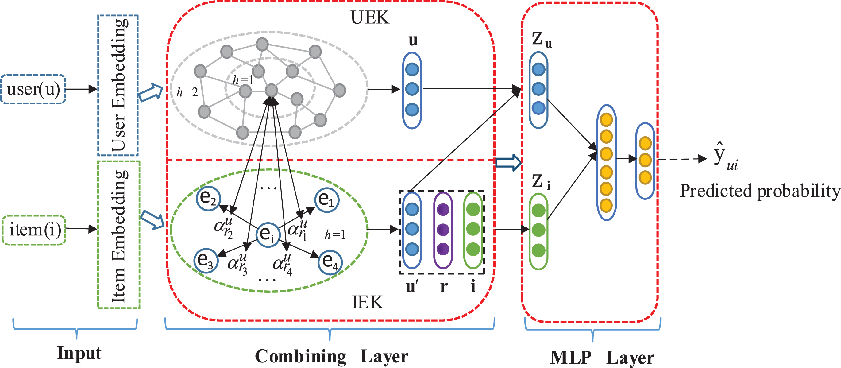
Overview of the proposed CUIKG. Overall, CUIKG consists of two key parts: a combined layer and an MLP layer.

3.3 Combining layer

User-end KG learning (UEK). Typically, in a personalized recommendation, the construction of user profiles is used to label a user, and this label is a highly refined feature characteristic that comes from the analysis of user information (user’s social attributes, living habits and consumption behaviour, etc.). Most existing methods are based on the discrete features extracted by hand, which cannot describe the context information of user data; thus, the representation ability for users is limited. In this study, we assume that most various information associated with users can be built into a knowledge graph. For example, MovieLens-20 M contains user attribute information. An example of user dataset is shown in Table 2.

Table 2
Sample of user data in MovieLens-20 M

UserID Gender Age Occupation Zip-code

1 F 18 10 48067

2 M 56 16 70072

3 M 25 15 55117

4 M 54 7 02460

UserID	Gender	Age	Occupation	Zip-code
1	F	18	10	48067
2	M	56	16	70072
3	M	25	15	55117
4	M	54	7	02460

In Table 2, userIDs are numbered from 1, with a total of 138159 users, and each user corresponds to a number. Gender is categorized as F for female and M for male. Age is the minimum value of each age range, and a total of 7 age ranges are divided into 1∼18, 18∼24, 25∼34, 35∼44, 45∼49, 50∼55, and 56+. Each number corresponds to an occupation, and there are 21 occupations in total, ranging from 0 to 20. Zip code represents the real zip code of the user’s location. Due to the large number of users, users with a movie score below 4 were filtered out during model building, while no threshold was set for Yelp. Each user was then renumbered, and an item and user knowledge graph was constructed based on the KG rule defined in Section 3.1. We performed the same method with the Yelp dataset and built the user-end KG.

After building the user-end KG, we removed the attribute relationship between entities because we only focus on learning the embedding of users; thus, we treat the KG as an undirected graph. Considering a candidate pair of user and item (u_l, i_j), in the UEK, as shown in the top half of combining layer, which yields an illustrative example of two-layer receptive field for a given user entity, we first obtain the user’s initial embedding $u_{l}$ by looking up the matrix E_U. Then, we sample the target user $u_{l}^{'} s$ neighbours from layers 1 to H as it is receptive field; the specific neighbour sampling strategy is shown in part 4.1. We denote N^h (u_l) as the h-hop neighbourhood set of the user u_l in user-end graph, then calculating the user representation by iteratively aggregating h-layer neighbourhood information via graph convolution. Concurrently, these embeddings are learned as well as the parameters of the GCNs. The embedding of target user u_l after h-layer convolution is: $h_{u_{l}}^{h} = Re LU (W_{u_{l}}^{h} • [h_{u_{l}}^{h - 1}; h_{N^{h} (u_{l})}^{h - 1}]), h_{u_{l}}^{0} = u_{l}$ (2)

We use the currently popular rectified linear unit ReLU (x) = max(0, x) as the nonlinear activation function, where [;] represents concatenation, and $W_{u_{l}}^{h}$ is the transformation weight matrix shared across all user entities for the target user in layer h. $h_{N^{h} (u_{l})}^{h - 1}$ is the neighbourhood embedding of the target user in layer h. To achieve the permutation invariance of each neighbour in the neighbourhood, the element-weighted average aggregator is used in this study to aggregate the neighbour information of each layer. The formula for calculating the aggregation of neighbour information of each layer is: $h_{N^{h} (u_{l})}^{h - 1} = {aggregator}^{h} ({h_{u}^{h - 1} : u \in N^{h} (u_{l})})$ (3)

${aggregator}^{h} = σ (MEAN ({Q_{u}^{h} • h_{u}^{h - 1}, u \in N^{h} (u_{l})}))$ (4)

where the sigmoid function is defined as σ (x) = 1/(1 + exp(- x)); $Q_{u}^{h}$ is the layer-h (user) aggregator weight matrix, which is shared across all user nodes at layer h; and MEAN (·) denotes the mean of the embedding in the argument set.

Item-end KG learning (IEK). The bottom half of the combining layer shows the framework of IEK. We constructed the item-end knowledge graph based on the two datasets and is also the same interaction pair (u_l, i_j) given in UEK, although we use GCNs both to learn the embeddings of users and items, the difference with UEK is that we aggregate the neighbourhoods information of the given item i_j based on the user $u_{l}^{'} s$ preference for the relationship between items. Thus, to consider the relevance between the user and the item, e_{N^h(e_{i
_j})} represents the collection of neighbours that directly connected to entity e_{i
_j} in layer-h; r_{e_{i
_j},e} represents the relationship between e_{i
_j} and it is each neighbour e ∈ e_{N^h(e_{i
_j})} in layer-h; and a score $α_{r_{e}}^{u_{l}}$ indicates the importance of relations r_{e_{i
_j},e} to u_l. The score is calculated by function φ (i.e., the inner product): $α_{r_{e}}^{u_{l}} = φ (u_{l}, r_{e})$ (5) where $u_{l} = h_{u_{l}}^{H}$ is $u_{l}^{'} s$ embedding learned from UEK, and r_e ∈ R^{d
_r} is the representation of relations corresponding r_{e_{i
_j},e}. After calculating the score between u_l and each relation, we use the calculated scores to combine the neighbours of e_{i
_j} linearly. The sampling strategy of each neighbour is the same as that of UEK, and the layer-h neighbourhood embedding $v_{N^{h} (e_{i_{j}})}^{h - 1}$ of the target entity e_{i
_j} can be represented as: $v_{N^{h} (e_{i_{j}})}^{h - 1} = \sum_{e \in N^{h} (e_{i_{j}})} {\tilde{α}}_{r_{e_{i_{j}}, e}}^{u_{l}} e$ (6) ${\tilde{α}}_{r_{e_{i_{j}}, e}}^{u_{l}} = \frac{exp (α_{r_{e_{i_{j}}, e}}^{u_{l}})}{\sum_{e \in N (e_{i_{j}}^{k - 1})} exp (α_{r_{e_{i_{j}}, e}}^{u_{l}})}$ (7) where e is the representation of entity e and ${\tilde{α}}_{r_{e_{i_{j}}, e}}^{u_{l}}$ is the layer-h normalized user-relation score. Similarly, the layer-h embedding of target item entity e_{i
_j} can be generated using another set of transformation and weight matrices:

$h_{e_{i_{j}}}^{h} = Re LU (W_{e_{i_{j}}}^{h} • [h_{e_{i_{j}}}^{h - 1}; v_{N^{h} (e_{i_{j}})}^{h - 1}]), h_{e_{i_{j}}}^{0} = e_{i_{j}}$ (8)

The advantage of this method is that we use embedding, which can capture the user’s profile to calculate the degree of preference for the relationship, to further mine the user’s potential interest and motivation. For example, in the movie recommendation scenario, a user may like the “Star” or the “director” of the movie. We think that by calculating the user’s score on the movie attribute, we can obtain the weight of aggregating the neighbour information of each item. However, there is a problem in this method. If the initial state of the user’s embedding is randomly initialized, it will lead to uncertainty in the score. In a real-world scenario, each user is described by a lot of attribute information, such as gender, age, and occupation, which constitute the user’s personal profile. Because each user’s profile is different, each user will have a different motivation for their movie preferences. For example, user A and user B score the same movie as 5 out of 10. User A may like the “type” of the movie, and the score calculated by user A for the “type” relationship will be significantly higher than that calculated by other relationships. However, user B may like the “Star” of the movie; thus, the score calculated by user B for the “Star” relationship will be significantly higher than that calculated by other relationships. Although the two users provide the same rating of the movie, we must more accurately mine the potential personalized preferences of users.

3.4 MLP layer

Under the input of the given formalization, we jointly train user-end KG and item-end KG. In terms of UEK, the ultimate output in the UEK section is $u_{l}^{'} s$ embedding u. In the IEK part, $u_{l}^{'} s$ embedding will also be output as well as the relations representation r and item embedding i. To distinguish $u_{l}^{'} s$ embedding of UEK partial output, we use u′ to represent $u_{l}^{'} s$ embedding learned from IEK. Based on the experience of previous researchers, the final user representation Z_u could be the average or concatenation of u and u′: $Z_{u} = θ u + (1 - θ) u^{'} or Z_{u} = [θ u; (1 - θ) u^{'}]$ (9) where θ is an adjustable parameter to control the weight of these two user embeddings. In the experiments, we compare the advantages and disadvantages of the two patterns, and the final item’s embedding Z_i is directly use i learned from UEK.

Once the final embedding of user u_l and item i_j are determined from the combining layer, we use several layers of a neural network that can fit any nonlinear function to deeply model the interactions among users and items. First, we merge the aforementioned user and item embeddings by embedding concatenation and feed them into a preference layer P that contains multiple feed-forward neural networks:

$p^{q} (z) = Re LU (W^{q} p^{q - 1} (z) + b^{q}), q \in [1, Q - 1]$ (10)

where the total number of hidden layers P is Q; the q-th hidden layer of P is denoted as p^q (z); p⁰ (z) = z = [Z_u ; Z_i] is the input layer of the entire neural network; W^q and b^q are the weight and bias of layer q, respectively; and the training of preference prediction ${\hat{y}}_{u_{l} i_{j}}$ yielded by the sigmoid layer on the top of P is leveraged to learn user preference over item: ${\hat{y}}_{u_{l} i_{j}} = σ ((ω^{Q})^{T} p^{Q - 1} (z))$ (11) where ω ^Q is the weight vector of the last layer. Second, to maintain a stable decrease in the classical GD and the stochastic characteristics of SGD concurrently, we use minibatch gradient descent to update the parameters of the proposed model. Then, we minimize the following loss function:

$\begin{matrix} L = log p (y | Θ) = - \sum_{(u_{i}, i_{j}) \in O^{+}} y_{u_{l} i_{j}} log ({\hat{y}}_{u_{l} i_{j}}) \\ - \sum_{(u_{i}, i_{j}) \in O^{-}} (1 - y_{u_{l} i_{j}}) log (1 - {\hat{y}}_{u_{l} i_{j}}) + \frac{λ}{2} {∥ Θ ∥}_{2}^{2} \end{matrix}$ (12) where L is the sigmoid cross-entropy loss; y is the set of labels of training pairs; O⁺ = {(u_l, i_j) |x_{u
_l
i
_j} = 1 and O^- = {(u_l, i_j) | x_{u
_l
i
_j} = 0} are the positive and negative user-item interaction pairs, respectively; and the last term of the formula is L2 regularization on the trainable parameters Θ to avoid overfitting.

The model parameters are trained by formulae (1) ∼ (12). Every time the minibatch samples are trained, the model parameters are updated, and the feature matrix of users and items is updated concurrently. During back propagation, the gradient of ∂L/∂E_U and ∂L/∂E_I is calculated based on the loss function L and updated by the learning rate η: $E_{U} = E_{U} - η \partial L / \partial E_{U}$ (13) $E_{I} = E_{I} - η \partial L / \partial E_{I}$ (14)

4 Experiments

In this section, quantitative experiments on top-K recommendation and click-through rate (CTR)recommendation tasks are performed. For each recommendation task, the MovieLens-20 M and Yelp datasets are used to verify the performance of UIKG. Additionally, the control variable method is also used to analyse the influence of hyperparameters on the model to select the most appropriate parameters and make the model achieve better performance in the recommended application scenarios. All experimental code and datasets are located at https://github.com/xiaoliangshare/ACM-RecSys.git. We invite researchers to contact us for help in implementing this code.

4.1 Dataset

Two real datasets, MovieLens-20 M and Yelp, are used to evaluate the proposed model. These datasets are the most widely used public datasets in the field of machine learning algorithms and recommendation systems. For each dataset, because the rating data in the original dataset belong to explicit feedback, we transform the rating data into implicit feedback. During data processing, records with each user rating below 4 are filtered in MovieLens-20 M and no users are filtered in Yelp. After processing, each record is marked as 1, which indicates that the user rating of the item is positive. A non-interactive item collection is sampled for each user. Each record is marked as 0, indicating that the user rating of the item is negative. Also, the proportion of each user rating positive items to negative rating items is 1:1.

^·MovieLens - 20 M : a widely used benchmark dataset in movie recommendation, which contains 20 million ratings from 138,159 users to 16,954 movies.

^·Yelp : this dataset records 799956 interactions between 32163 users and 57159 local businesses and contains user profiles (e.g., ID, review count and fans) and item attributes (e.g., ID, city and stars).

Based on user attribute information and item meta-data information stored in the two datasets, we use Microsoft Satori to build the user and item knowledge graphs, respectively. The basic statistical information of the datasets is shown in Table 3.

Table 3
Basic statistics of dataset

Movie Lens-20 M Yelp

User-Item Interactions #Users 138159 32163

#Items 16954 57159

#Interactions 13501622 799956

#Avg.Interactions 97 245

#Sparsity 95.5% 91.9%

User KG #User Entities 147667 65626

#User Relations 4 4

#User Triple 241440 128656

Item KG #Item Entities 102569 57200

#Item Relations 32 4

#Item Triple 499474 285795

		Movie Lens-20 M	Yelp
User-Item Interactions	#Users	138159	32163
	#Items	16954	57159
	#Interactions	13501622	799956
	#Avg.Interactions	97	245
	#Sparsity	95.5%	91.9%
User KG	#User Entities	147667	65626
	#User Relations	4	4
	#User Triple	241440	128656
Item KG	#Item Entities	102569	57200
	#Item Relations	32	4
	#Item Triple	499474	285795

4.2 Experimental settings

Python 3.7.3 and TensorFlow 1.14.0+ numpy1.14.3 are used in the experiment. The ratio of the training set, verification set and test set is 7:1:2. The initial values of the hyperparameters are set in the experiment without pretraining. For all models, we use the Adaptive Moment Estimation (Adma) and Adagrad as optimizers, and apply a grid search to the models to find the best settings for each task. The search range of learning rate η is {0.001, 0.002, 0.005, 0.01, 0.02}, and the coefficient of L2 regularization is {10–5, 10–4, 10–3, 10–2, 10–1, 0}. The weight factor θ of the user embedding output by UEK and IEK is set to 0.5, and the embedding of the end user is obtained by concatenation by default. The default value of the number of layers Q of preference layer P is set to 1, which is input layer ⟶hidden layer⟶output layer. For simplicity, the embedding dimension of users and items is set to d = du = di = 32, and the corresponding embedding dimension of each layer is 64⟶32⟶1. The number of iterations (epochs) of each experiment is set to 10, and the number of training samples (batch-size) is 65536. Each experiment was repeated three times, and mean results are reported. L2 regularization and dropout technology are used during training to prevent overfitting. The default depth H of the local receptive field is 3. The size of neighbours aggregated in each layer is S, and the default value is set to 8. The neighbour sampling strategy of each layer is described as follows. First, for a given entity in the user (item) knowledge graph, there may be multiple neighbours directly connected to the entity; if both are aggregated, the calculation efficiency is lower. To keep the computational pattern of each batch and the calculation efficiency fixed, we select S neighbours from all neighbours of the entity for aggregation. If the number of all neighbours of a given entity is greater than S, the S neighbours are randomly selected from all neighbours of the entity. If the number of all neighbours of a given entity is below S, there are only s (s < S) neighbours, and we randomly copy (S-s) neighbours from s to S. Because these experiments and a comparison method are based on the same dataset standard, the experimental parameters of a comparison methods are set to the default values given by their original papers.

4.3 Baselines

There are two types of representative comparison methods in this study: recommendation methods (SVD, libFM) without a knowledge graph, and recommendation methods (libFM+TransE, CKE, RippleNet, KGCN) that use a knowledge graph to learn the user (item) embedding. The following methods are compared to the proposed model:

SVD [34] is a classic method based on collaborative filtering. The basic principle of SVD is that every matrix has full rank decomposition. Two matrices _U and _V are obtained by training the user-item rating matrix _X decomposition, and unknown scores are obtained by the dot product of a row of _U and a column of _V.

LibFM [35] is a general method that simulates most decomposition models by feature engineering that is developed from SVD models. There are only two types of features in the SVD model: user features and item features, and the LibFM model can contain several types of these features.

LibFM + TransE introduces the knowledge graph. The core function of the TransE model is to translate the triples in the knowledge graph into a representation vector and attach the learned item representation vector to the item representation vector on the libFM model.

CKE [36] uses a knowledge base to design three components to extract semantic representations of items from structural, text and visual content. Then, a collaborative knowledge base embedding (CKE) integration framework is proposed. In this framework, Bayesian TRANSR, Bayesian SDAE and Bayesian SCAE jointly learn potential representations in collaborative filtering and semantic representations of items in knowledge graphs.

RippleNet [26] is a type of neural network that combines a knowledge graph and recommendation system. This network populates user’s interest preferences in a knowledge graph and gradually attenuates user preferences during continuous diffusion, which is similar to the function of a memory network.

KGCN [27] uses a multilayer convolution method to determine the item knowledge graph. The user preference for an item is obtained by the dot product of user embedding and item embedding but does not construct a user profile.

4.4 Evaluation metrics

After several training iterations, we can determine whether model training is complete by observing the change in the loss function value. When its value is near 0 and tends to be flat, model training is considered complete. Then, the trained model is used for prediction. The same evaluation metrics are used to evaluate the proposed method and comparison methods in this paper. Based on different recommendation tasks, the evaluation metrics used in this experiment are as follows:

In Top-K recommendation, for each given test user, all items that the user has interacted within the test set are considered to be the truth set ground_truth_items, and then the preference probabilities of the user with all items that the user has not interacted with are calculated. We sort the probability value and select the top_k item set with the highest probability recommended to users as a candidate set. Recall@K is used in this study to evaluate the recommendation performance of the model. Recall@K represents how many items in top_k belong to the ground_ truth_ items. The formula of Recall@K is as follows: $Rec @ K = \frac{ground_truth_items ⋂ top_k}{ground_truth_items}$ (13)

Finally, the average value of all users Recall@K is calculated as the final metric value.

In CTR prediction, F1 and AUC are used to evaluate the performance of the model. F1 represents the mean value of the Precision@K and Recall@K of the model; Precision@K indicates how many items in the ground_ truth_ items belong to top_k; and AUC represents the area under the ROC curve which is a curve composed of false positive rate as abscissa and true positive rate as ordinate. Precision@K and F1 are calculated as follows:

Pre @ K = \frac{ground_truth_items ⋂ top_k}{top_k}

(14)

F 1 = \frac{2 * Rec @ K * Pre @ K}{Rec @ K + Pre @ K}

(15)

Similarly, the average F1 of all users is calculated as the final metric value.

4.5 Experimental results and analysis

4.5.1 Experimental results recommended by Top-K

The result of the Top-K recommendation is shown in Fig. 2, which shows a comparison curve of the proposed method and comparison methods (CKE, libFM+TransE, RippleNet, KGCN). Because SVD and libFM directly calculate the score to represent the user’s preference for the item, their curves are not drawn. The abscissa of Fig. 2 represents the number of items in top_k, and the ordinate represents the recall@K corresponding to K. Figure 2 shows that CUIKG outperforms the baseline methods by 3.0% ∼20.5% under the metric of recall@K in Yelp but only increases by 2.5% ∼13.6% in MovieLens-20 M. By incorporating KG, CUIKG yields more promising improvements on Yelp than MovieLens-20 M, which implies that the knowledge graph is more helpful for sparse data. Figure 2 also shows that KGCN and RippleNet yield good performance on the two datasets primarily because they use GCN to model the items and users, respectively, on the knowledge graph. Due to their lack of consideration of the impact between users and items when generating their respective representations, their performance is not as good as UIKG. Lastly, Fig. 2 also shows that although libFM+TransE and CKE also introduce the knowledge graph as auxiliary information, their learning model of the knowledge graph is based on the translation distance model or semantic matching model, which is more suitable for link completion and link prediction of the knowledge graph. Therefore, the performance in the recommendation scenario is more general, which verifies that the method based on GCN can extract features of users and items more effectively.

Fig. 2

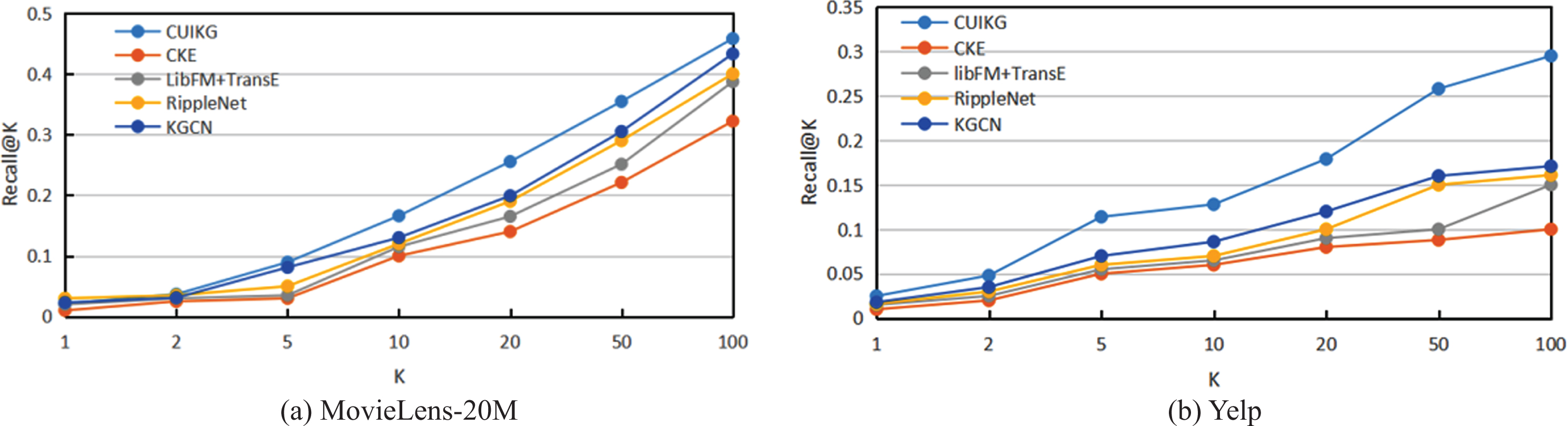
Recall@K in Top-K recommendation.

4.5.2 Experimental results recommended by CTR

The AUC and F1 metric values under the CTR recommendation scenario are shown in Table 4. Results show that the performance of the proposed method is optimal on both datasets. Compared to the contrast methods, the performances of SVD and libFM without a knowledge graph are better than that of CKE, which indicates that the CKE method cannot make good use of the knowledge graph as auxiliary information for modelling. However, their performance is worse than that of RippleNet, KGCN and UIKG. This situation is similar to the Top-K recommended scenario, indicating that the GCN-based method can effectively model the interaction between users and items. Also, LibFM+TransE performs better than LibFM in most cases, which demonstrates that introducing a knowledge graph into the recommendation system can improve model performance. Lastly, compared to MovieLens-20 M, the proposed model performs better on Yelp, and the improvements are similar to those on Top-K recommendation.

Table 4
AUC and F1 in CTR prediction

Model MovieLens-20 M Yelp

AUC F1 AUC F1

SVD 0.963 (–1.9%) 0.919 (–3.4%) 0.671 (–11.1%) 0.652 (–10.7%)

LibFM 0.959 (–2.3%) 0.906 (–4.7%) 0.663 (–11.9%) 0.649 (–11.0%)

LibFM+TransE 0.966 (–1.6%) 0.917 (–3.6%) 0.699 (–8.3%) 0.663 (–9.6%)

CKE 0.924 (–5.8%) 0.871 (–8.2%) 0.655 (–12.7%) 0.641 (–11.8%)

RippleNet 0.968 (–1.4%) 0.912 (–4.1%) 0.722 (–6.0%) 0.693 (–6.6%)

KGCN 0.978 (–0.4%) 0.932 (–2.1%) 0.747 (–4.4%) 0.705 (–5.4%)

UIKG 0.982 0.953 0.762 0.759

Model	MovieLens-20 M	Yelp
SVD	0.963 (–1.9%)	0.919 (–3.4%)	0.671 (–11.1%)	0.652 (–10.7%)
LibFM	0.959 (–2.3%)	0.906 (–4.7%)	0.663 (–11.9%)	0.649 (–11.0%)
LibFM+TransE	0.966 (–1.6%)	0.917 (–3.6%)	0.699 (–8.3%)	0.663 (–9.6%)
CKE	0.924 (–5.8%)	0.871 (–8.2%)	0.655 (–12.7%)	0.641 (–11.8%)
RippleNet	0.968 (–1.4%)	0.912 (–4.1%)	0.722 (–6.0%)	0.693 (–6.6%)
KGCN	0.978 (–0.4%)	0.932 (–2.1%)	0.747 (–4.4%)	0.705 (–5.4%)
UIKG	0.982	0.953	0.762	0.759

4.6 Influence of hyperparameters on UIKG

The following section analyses the influence of hyperparameters on the experimental results. We only examine the influence of hyperparameters on the experimental results in the CTR recommendation scenario.

Impact of the number of hidden layers in the MLP layer: The following conclusions can be drawn from Table 5. First, as the number of hidden layers increases, the performance of the model improves. When the hidden layer increases from 0 to 2, in MovieLens-20 M, the AUC metric increases by 0.3% and 0.2%, and the F1 metric decreases by 0.5% and increases by 0.8%; in Yelp, the AUC increases by 1.1% and 2.0%, and the F1 metric increases by 1.8% and 6.5%, respectively. Finally, the performance exhibits an upward trend, which indicates the effectiveness of using the expressive neural networks for modelling user preference. The marginal decline may be caused by data fluctuation due to the large number of training samples, and each iteration of training will shuffle the samples randomly before training, which will lead to certain data fluctuations. Second, when the number of hidden layers increases from 2 to 3, the performance of the model decreases markedly. Compared to the results with 2 layers, the AUC and F1 metric decreased by 1% and 1.6%, respectively, in the MovieLens-20 M dataset, and there was also a downward trend in the Yelp dataset, which shows that when the hidden layer is too high, the fitting ability of the neural network to function is increased. However, concurrently, the complexity of the model is also increased and results in an overfitting phenomenon, which results in the expression ability of the test set being decreased.

Table 5
AUC and F1 result of CUIKG with different Q

Q 0 1 2 3

MovieLens-20 M AUC 0.982 0.985 0.987 0.977

F1 0.954 0.959 0.957 0.941

Yelp AUC 0.751 0.762 0.782 0.766

F1 0.696 0.714 0.779 0.758

Q	0	1	2	3
MovieLens-20 M	AUC	0.982	0.985	0.987	0.977
	F1	0.954	0.959	0.957	0.941
Yelp	AUC	0.751	0.762	0.782	0.766
	F1	0.696	0.714	0.779	0.758

Impact of dimensions of embedding: Table 6 shows that increasing the dimension of the embedding can improve the expression performance of the model, indicating that the model performance can be improved by appropriately increasing the number of features. However, when the threshold exceeds a certain value, overfitting will tend to occur in the model. From the experimental results, CUIKG achieves the best performance when d = 32 on both datasets.

Table 6

AUC and F1 result of CUIKG with different d

d	16	32	64	128
MovieLens-20 M	AUC	0.981	0.982	0.980	0.975
	F1	0.950	0.953	0.952	0.865
Yelp	AUC	0.757	0.798	0.796	0.791
	F1	0.707	0.736	0.731	0.728

Impact of depth H of the local receptive field: Based on the experimental results in Table 7, the performance of the model is best when H = 1. When H is 2 and 3, although performance decreases, the performance remains strong. With increasing local receptive field depth, the performance of the model results also declined. Particularly when H = 4, the performance of the model decreases markedly. When H equalled 5, 6, and 7, the performance of the model gradually decreased, which also shows that increasing the depth of GCN will cause model performance to gradually decline due to excessive smoothing.

Table 7

AUC and F1 result of CUIKG with different H

H	1	2	3	4
MovieLens-20 M	AUC	0.986	0.982	0.980	0.975
	F1	0.957	0.953	0.952	0.865
Yelp	AUC	0.771	0.768	0.760	0.746
	F1	0.752	0.749	0.737	0.702

Impact of the number of sampled neighbours S: Based on the experimental results in Table 8, model performance increases as S increases. When S equals 8, the aggregated neighbour information is sufficient to represent the information of the target entity. However, as S continues to increase, the neighbour information may aggregate into unnecessary noisy neighbours, which will lead to a decline in model performance.

Table 8

AUC and F1 result of CUIKG with different S

S	₂	₄	₈	₁₆
MovieLens-20 M	AUC	0.980	0.981	0.982	0.982
	F1	0.952	0.954	0.955	0.953
Yelp	AUC	0.782	0.788	0.796	0.785
	F1	0.733	0.739	0.740	0.729

5 Conclusion

This paper describes the learning of user-_end item-end knowledge graphs. The purpose of learning the user-end knowledge graph is to construct user profiles. Then, we introduce the learned embedding of the user into the item-end knowledge graph learning to mine the motivation behind the users’ engaging the item. The proposed model can capture the relevance between users and items, which shows user preferences for consuming items. The experimental results show that the CUIKG framework outperforms existing methods on the MovieLens-20 M and Yelp datasets by 2.5% ∼13.6% under the metric of recall@K and a 0.4% ∼11.9% increase in AUC and F1 indicators. These results show that the proposed method can enhance the representation of users and items, and model user preferences better than other personalized recommendation methods.

In the future, we plan to introduce more user attributes to improve the depth of user profiles. Due to the high computational complexity of knowledge graph training, optimizing the model and considering the application of the model in a real-world scenario will be studied in more detail. In real-world scenarios, users’ preferences can be interfered from social networks in real time. The method proposed in this paper is suitable for static knowledge graphs; however, if new knowledge is added, we will consider combining users’ social networks to capture their friends’ long-term preferences to capture users’ dynamic interest changes.

Footnotes

Acknowledgments

This work was partially supported by the National Natural Science Foundation of China (Nos. 62066010,61862016,61966009), the Natural Science Foundation of Guangxi Province (No. 2020GXNSFAA159055), and the Guangxi Innovation-Driven Development Grand Project (No. AA17202024).

References

Lian

, Zheng

V.W.

and Xie

, Collaborative filtering meets next check-in location prediction, WWW (Companion Volume), 2013, 231–232.

Rendle

, Gantner

and Freudenthaler

, Lars Schmidt-Thieme: Fast context-aware recommendations with factorization machines, SIGIR 2011, 635–644.

Gao

, Tang

, Hu

and Liu

, Content-Aware Point of Interest Recommendation on Location-Based Social Networks, AAAI 2015, 1721–1727.

Huang

, Zhao

W.X.

, Dou

, Wen

J.-R.

and Chang

E.Y.

, Improving Sequential Recommendation with Knowledge-Enhanced Memory Networks, SIGIR 2018, 505–514.

Wang

, Zhang

, Xie

and Guo

, DKN: Deep Knowledge-Aware Network for News Recommendation, WWW 2018, 1835–1844.

Zhang

, Shi

, Zhao

and King

, STAR-GCN: Stacked and Reconstructed Graph Convolutional Networks for Recommender Systems, IJCAI 2019, 4264–4270.

Gao

, Tang

, Hu

and Liu

, Content-Aware Point of Interest Recommendation on Location-Based Social Networks, AAAI 2015, 1721–1727.

, Ren

, Sun

, Gu

, Sturt

, Khandelwal

, Norick

and Han

, Personalized entity recommendation: a heterogeneous information network approach, WSDM 2014, 283–292.

Zhao

, Yao

, Li

, Song

and Lee

D.L.

, Meta-Graph Based Recommendation Fusion over Heterogeneous Information Networks, KDD 2017, 635–644.

10.

Chen

, Xu

, Zhang

, Tang

, Cao

, Qin

and Zha

, Sequential Recommendation with User Memory Networks, WSDM 2018, 108–116.

11.

and Chua

T.-S.

, Neural Factorization Machines for Sparse Predictive Analytics, SIGIR 2017, 355–364.

12.

, He

, Du

and Chua

T.-S.

, Adversarial Personalized Ranking for Recommendation, SIGIR 2018, 355–364.

13.

, Zhao

, Zhang

, Zhu

, Xiao

and Wang

, Improved Deep Walk Algorithm Based on Preference Random Walk, NLPCC (1) 2019, 265–276.

14.

Lazaridou

, Pham

N.T.

and Baroni

, Combining Language and Vision with a Multimodal Skip-gram Model, HLT-NAACL 2015, 153–163.

15.

Tang

, Qu

, Wang

, Zhang

, Yan

and Mei

, LINE: Large-scale Information Network Embedding, WWW 2015, 1067–1077.

16.

Grover

and Leskovec

, node2vec: Scalable Feature Learning for Networks, KDD 2016, 855–864.

17.

Q.V.

and Mikolov

, Distributed Representations of Sentences and Documents, ICML 2014, 1188–1196.

18.

Bordes

, Usunier

, García-Durán

, Weston

and Yakhnenko

, Translating Embeddings for Modeling Multi-relational Data, NIPS 2013, 2787–2795.

19.

Lin

, Liu

, Sun

, Liu

and Zhu

, Learning Entity and Relation Embeddings for Knowledge Graph Completion, AAAI 2015, 2181–2187.

20.

Zhang

, Shi

, Zhao

and King

, STAR-GCN: Stacked and Reconstructed Graph Convolutional Networks for Recommender Systems, IJCAI 2019, 4264–4270.

21.

Wang

, Wang

, Xu

, He

, Cao

and Chua

T.-S.

, Explainable Reasoning over Knowledge Graphs for Recommendation, AAAI 2019, 5329–5336.

22.

Ying

, He

, Chen

, Eksombatchai

, Hamilton

W.L.

and Leskovec

, Graph Convolutional Neural Networks for Web-Scale Recommender Systems, KDD 2018, 974–983.

23.

Chami

, Ying

, Ré

and Leskovec

, Hyperbolic Graph Convolutional Neural Networks, Neur IPS 2019, 4869–4880.

24.

Zhang

, Yuan

N.J.

, Lian

, Xie

and Ma

W.-Y.

, Collaborative Knowledge Base Embedding for Recommender Systems, KDD 2016, 353–362.

25.

Guo

, Wang

and Guo

, Semantically Smooth Knowledge Graph Embedding, ACL (1) 2015, 84–94.

26.

Wang

, Zhang

, Wang

, Zhao

, Li

, Xie

and Guo

, RippleNet: Propagating User Preferences on the Knowledge Graph for Recommender Systems, CIKM 2018, 417–426.

27.

Wang

, Zhao

, Xie

, Li

and Guo

, Knowledge Graph Convolutional Networks for Recommender Systems, WWW 2019, 3307–3313.

28.

Wang

, He

, Cao

, Liu

and Chua

T.-S.

, KGAT: Knowledge Graph Attention Network for Recommendation, KDD 2019, 950–958.

29.

Wang

, Mao

, Wang

and Guo

, Knowledge Graph Embedding: A Survey of Approaches and Applications, IEEE Trans Knowl Data Eng 29(12) (2017), 2724–2743.

30.

Bruna

, Zaremba

, Szlam

and Cun

Y.L.

, Spectral Networks and Locally Connected Networks on Graphs, ICLR (2014).

31.

Defferrard

, Bresson

and Vandergheynst

, Convolutional Neural Networks on Graphs with Fast Localized Spectral Filtering, NIPS 2016, 3837–3845.

32.

Hamilton

W.L.

, Ying

and Leskovec

, Inductive Representation Learning on Large Graphs, NIPS 2017, 1024–1034.

33.

Velickovic

, Cucurull

, Casanova

, Romero

, Liò

and Bengio

, Graph Attention Networks, CoRR abs/1710.10903 (2017).

34.

Koren

, Factorization meets the neighborhood: a multifaceted collaborative filtering model, KDD 2008, 426–434.

35.

Rendle

, Factorization Machines with libFM, ACM Trans Intell Syst Technol 3(3) (2012), 57:1–57:22.

36.

Zhang

, Yuan

N.J.

, Lian

, Xie

and Ma

W.-Y.

, Collaborative Knowledge Base Embedding for Recommender Systems, KDD 2016, 353–362.

37.

Xian

, Fu

, Muthukrishnan

, de Melo

and Zhang

, Reinforcement Knowledge Graph Reasoning for Explainable Recommendation, SIGIR 2019, 285–294.

38.

Monti

, Bronstein

M.M.

and Bresson

, Geometric Matrix Completion with Recurrent Multi-Graph Neural Networks, NIPS 2017, 3697–3707.

39.

, Wu

, Mao

, Wang

and Zhang

, Recommender system application developments: A survey, Decis Support Syst 74 (2015), 12–32.

40.

Zhao

, Zhou

, Guan

, Zhao

, Ning

, Qiu

and He

, Intent GC: A Scalable Graph Convolution Framework Fusing Heterogeneous Information for Recommendation, KDD 2019, 2347–2357.

41.

, Deng

, Wang

, Li

, Zhang

Y.-D.

and Wang

, LightGCN: Simplifying and Powering Graph Convolution Network for Recommendation, SIGIR 2020, 639–648.

42.

Wang

, Lian

and Ge

, Binarized Collaborative Filtering with Distilling Graph Convolutional Networks, CoRR abs/1906.01829 (2019).

43.

Bobadilla

, Ortega

, Hernando

and Gutiérrez

, Recommender systems survey, Knowl Based Syst 46 (2013), 109–132.

Combining user-end and item-end knowledge graph learning for personalized recommendation

Abstract

Keywords

1 Introduction

2 Related work

2.1 Recommendation with GCNs

2.2 Knowledge-aware recommendation

3 Proposed method

3.1 Preliminaries

Table 2 Sample of user data in MovieLens-20 M UserID Gender Age Occupation Zip-code 1 F 18 10 48067 2 M 56 16 70072 3 M 25 15 55117 4 M 54 7 02460

4.1 Dataset

4.3 Baselines

4.4 Evaluation metrics

4.5.1 Experimental results recommended by Top-K

Table 5 AUC and F1 result of CUIKG with different Q Q 0 1 2 3 MovieLens-20 M AUC 0.982 0.985 0.987 0.977 F1 0.954 0.959 0.957 0.941 Yelp AUC 0.751 0.762 0.782 0.766 F1 0.696 0.714 0.779 0.758

Footnotes

Acknowledgments

References

Table 2
Sample of user data in MovieLens-20 M

UserID Gender Age Occupation Zip-code

1 F 18 10 48067

2 M 56 16 70072

3 M 25 15 55117

4 M 54 7 02460

Table 5
AUC and F1 result of CUIKG with different Q

Q 0 1 2 3

MovieLens-20 M AUC 0.982 0.985 0.987 0.977

F1 0.954 0.959 0.957 0.941

Yelp AUC 0.751 0.762 0.782 0.766

F1 0.696 0.714 0.779 0.758