Evaluation and prediction of free driving behavior type based on fuzzy comprehensive support vector machine

Abstract

Driving behavior type is a hotspot in transportation field, but there have been few studies on free driving behavior type. The factor of current driving behavior evaluation model is single, and its environmental adaptability is insufficient, and driving behavior type is difficult to predict accurately. In addition, free driving behavior as one kind of the important driving operation behaviors lacks quantitative assessment methods and models. In view of these deficiencies, evaluation and prediction of free driving behavior based on Fuzzy Comprehensive Support Vector Machine (FC-SVM) is proposed. Firstly, a variety of individual decision-making behavior data obfuscating with environmental complexity are collected. These obtained parameters were used as FC multi-factor evaluation parameters to quantitatively evaluate free driving behavior from multiple aspects, and to qualitatively derive the driver’s driving behavior type. Further, the SVM used the RBF kernel function to obtain the optimal parameters and train the SVM network, and it used the obtained SVM model for the prediction of driving behavior type in short time. The results of simulations using different methods show that the SD value of FC-SVM evaluation results is the lowest, only 1.273. Compared with other common methods, its MacroP reaches 89.2%. It is interesting to find that aggressive driving can be more distinct from other behavior types. Moreover, the mixed traffic flow composed of aggressive driver has a higher traffic efficiency in basic sections. This work is of great value for improving driving behavior, reducing road congestion and improving road traffic efficiency in the mixed intelligent traffic.

Keywords

Free driving behavior fuzzy comprehensive support vector machine evaluation and prediction intelligent system

1 Introduction

Road traffic accidents have become a major public health problem worldwide. According to the World Health Organization (WHO), more than 1.35 million people suffer from road traffic accidents in the world every year. In addition, between 20 and 50 million people have suffered non-fatal injuries, many of whom are disabled. For traffic violations, unsafe driving behavior is one of the main reasons. Free driving behavior, one of the most important driving behaviors, is of great research value in this aspect. The driver will form his own unique free driving behavior type duringthe long-term driving process, so deriving the specific free driving behavior type with the established model and predicting the driving behavior type in the next stage are beneficial to increasing the current road safety and traffic efficiency. In the future, intelligent transportation systems will consist of human driving and autonomous driving. Through vehicle-to-vehicle information interaction, free driving behavior types of the adjacent vehicles are obtained, and the current vehicle’s driving mode will be changed. This is of great value to improving the safety of mixed traffic flow, and alleviating traffic congestion.

There are many types of overall driving behavior evaluation models, but there are problems of single evaluation factors and perspectives, and environmental adaptability is not enough [1]. The evaluation of driving behavior is based on the driving behavior model, which is continuously deepened and improved. Ajzen proposed the TPB model, which did not take into account the behavior or habits of the driver in a certain period of the past [2]. Reason proposed the ACM model, which was on the environmental factors influencing the behavior, instead of focusing on the influence of factors brought by the behavior individual [3]. Verschuur and Hurts combined the ACM theory with the TPB theory and proposed the driver safety behavior model (SDBM), which also ignored the impact of driver personality traits and traffic environment changes on driving behavior [4]. In recent years, the research on driving behavior has still been concerned. Ping-fan Li constructed the driving behavior characterization index system from four aspects including perception, decision-making, control and vehicle running state [5]. Based on the influencing mechanism of human factors on road traffic accidents, Peng-fei Yang analyzed the main factors influencing safety of operating drivers on the basis of ACM theory, TPB theory and heinrich cause-and-effect linkage theory [6]. Taking driving safety as the research content, Yang Li just integrated the acquisition schemes of different attribute indexes to build the indexes and evaluation model representing driving safety, which didn’t consider other aspects comprehensively [7].

Free driving, car following and lane changing form all specific driving behaviors, which is an important basis in driving rule extraction based on cognitive behavior analysis [8]. Nowadays, more researches focus on car following behavior type and lane changing behavior type, but there have been few studies on free driving behavior type. Chai et al. [9] et al. measured the heart rate and other indicators of different drivers in the process of following by vehicle sensors, so as to further classify drivers. Woo H et al. [10] proposed a new classification method for drivers in the process of following. By analyzing the following characteristics of drivers in different scenes, they proposed the model to classify drivers into different types. Tian E [11] classified test drivers by acquiring lane change behavior data of 38 drivers and lane change time of each driver by K clustering hierarchical clustering analysis. The experimental results divided drivers into 5 types, from conservative to radical. Thomas Ayres [12] analyzed the visual characteristics of the driver during lane change and analyzed the driving behavior characteristics based on the data of the driver’s attention to the rearview mirror before lane change. Jin Mao [13] of Chang’an University established an adaptive lane change warning model and analyzed the experimental data through fuzzy mathematics theory to obtain the driving types of different drivers. Considering the interactions between different drivers, lane changing behaviors were classified as mandatory and free lane changing [14]. Car following behaviors were classified as passive following and active following. If the driving vehicle is closely followed by other vehicles, some drivers will choose to change lane, while some will choose to drive at the current lane. If the driver comes across the traffic lights, some drivers will choose to wait until the green light, while some will choose to run the red light. Faced with these situations, this kind of driving behavior is free and not be restricted. Recently, some scholars focused on characteristics of individual drivers and vehicles under complex vehicle situations [15]. There were scholars proposing methods to control lane changing and car following based on the optimal control [16]. However, free driving behavior is one kind of complex driving behaviors including free lane changing and free car following, which lacks quantitative assessment methods and models at present stage.

In view of few researches on free driving behavior type and single angles and inadequate environmental adaptability in evaluation, Fuzzy Comprehensive Evaluation Method (FC-EM), one of the main effective evaluation methods, is paid great attention to. It deals with fuzzy evaluation objects by precise numerical means and makes a more scientific and reasonable quantitative evaluation close to reality for the data containing fuzzy information. The evaluation results contain rich information, which can not only accurately depict the evaluated object, but also further process to obtain reference information. In addition, this method can comprehensively evaluate the things affected by many factors and combine fuzzy mapping with its mathematical model. This method not only provides an accurate scientific basis for the results that are difficult to quantify in real life, but also shows the relationship among qualitative and quantitative differences between different complex things [17, 18]. Therefore, a multi-factor driving behavior evaluation model based on fuzzy synthesis is proposed, which collects driver’s individual decision behavior data, senses many influencing factors such as the distance between the driver and other traffic participants. Besides, these factors are combined with environmental complexity. The model evaluates the driving behavior quantitatively and comprehensively from safety, comfort, economy and other aspect, which can obtain the driver’s free driving behavior type.

Intelligent driving has developed rapidly in recent years, and one of the core technologies in intelligent driving is intelligent control. When performing intelligent control, it is essential to consider the safety, comfort, economy and other factors of driving, so the prediction and the identification of the driving mode are crucial. Support Vector Machines (SVM) is a data mining method based on statistical learning theory. It is a kind of generalized linear classifier that classifies data by supervised learning method. SVM uses hinge loss function to calculate empirical risk and adds regularization term to the solving system to optimize structural risk. It is a classifier with sparsity and robustness. SVM, one of the common kernel learning methods, can be used for nonlinear classification by kernel method. It can successfully deal with many problems such as pattern recognition including classification problem and discriminant analysis. In recent years, many researches have demonstrated that the accuracy of identifying or predicting specific driving behavior based on SVM is higher than other methods. [19 –21]. However, the prediction of driving behaviors is targeted at overall driving behaviors, and there is few prediction of driver’s specific free driving behavior type. Therefore, this paper uses SVM to predict the behavior type of the driver’s free driving behavior in the next stage. Fuzzy mathematics and SVM are combined, and fuzzy comprehensive support vector machine is proposed to overcome the influence of noise and outliers on SVM [22, 23]. It has good performance advantages, but it hasn’t been applied to driving behavior classification. Therefore, this paper combines FC-EM based on fuzzy mathematics with SVM, that is, FC-SVM is applied to the field of driving behavior classification prediction.

At this stage, there are few researches on free driving behavior type and the factor of the current driving behavior evaluation model is single. Besides, the model’s environmental adaptability is inadequate and the driving behavior type is difficult to predict accurately. A free driving comprehensive evaluation and prediction method based on fuzzy comprehensive support vector machine (FC-SVM) is proposed to make up these deficiencies. Through large numbers of experiments, we can obtain some extra conclusions. In the mixed traffic flow, free driving behavior types of the adjacent vehicles are obtained after applying our proposed method, and the current vehicle’s driving mode will be changed. This is of great value to improving the safety of mixed traffic flow, and alleviating traffic congestion. In this paper, Section 2 provides the analysis of the evaluation system about free driving behavior. Section 3 establishes evaluation and prediction model of free driving behavior based on FC-SVM. Section 4 designs numbers of experiments to verify the advantages of the proposed method and further discuss our work’s application in mixed traffic flow. Section 5 provides conclusions and future work.

2 Analysis of the evaluation system about free driving behavior

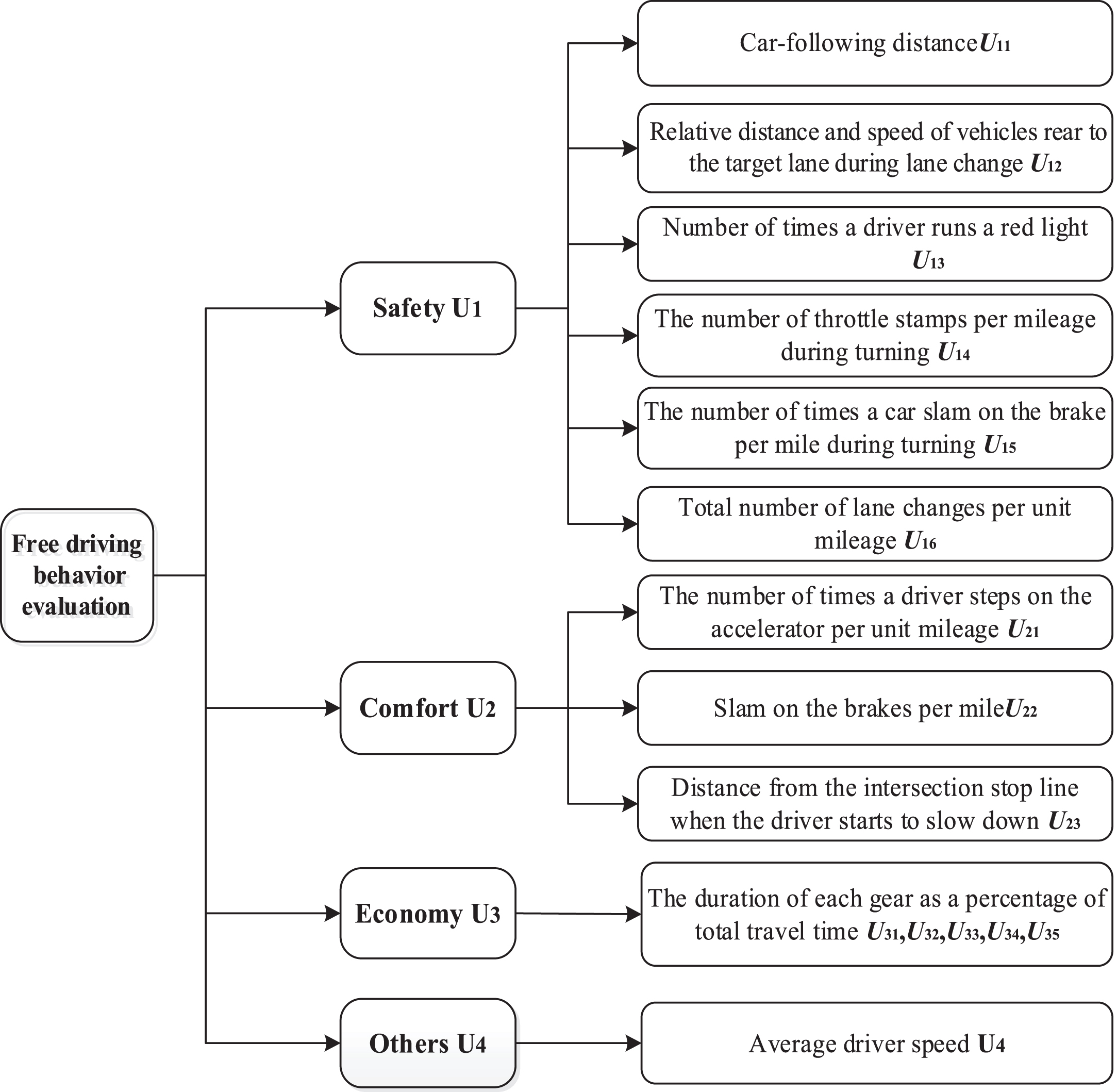
Before constructing the free driving behavior evaluation index system, we do the analysis of possible influencing factors in free driving. Drivers of different types choose different operations in free driving. In the view of safety point, many factors contribute to the final free driving type such as car-following distance, total number of lane changes, number of times a driver runs a red light, the number of times a car slam on the brake during turning and so on. In the view of comfort point, influencing factors include the number of times a driver steps on the accelerator and slam on the brakes and so on. From the point of economy, the duration of each gear as a percentage of total travel time should be considered. After that, choosing the right evaluation indicators is the key to the success of the evaluation model. A plurality of evaluation indicators can characterize various characteristics and relationships of the evaluated objects, thereby constituting an integral with an internal structure. In general, the establishment of the evaluation indicator system should follow the following principles: (1) the principle of typicality; (2) the principle of dynamics; (3) the principle of comparability; (4) the principle of testability; (5) concise scientific principles. According to the scientificity and feasibility of the evaluation index system in literature [7 , 24–26], a relatively perfect evaluation index system of free driving behavior is established in combination with the actual situation, as shown in Fig. 1 above. The first-level indicators include safety U₁, comfort U₂, economy U₃ and others U₄. Further, the first-level indicators include their own secondary indicators. Specially, the average speed is used to evaluate the others indicator.

Fig. 1

Free Driving behavior evaluation index system.

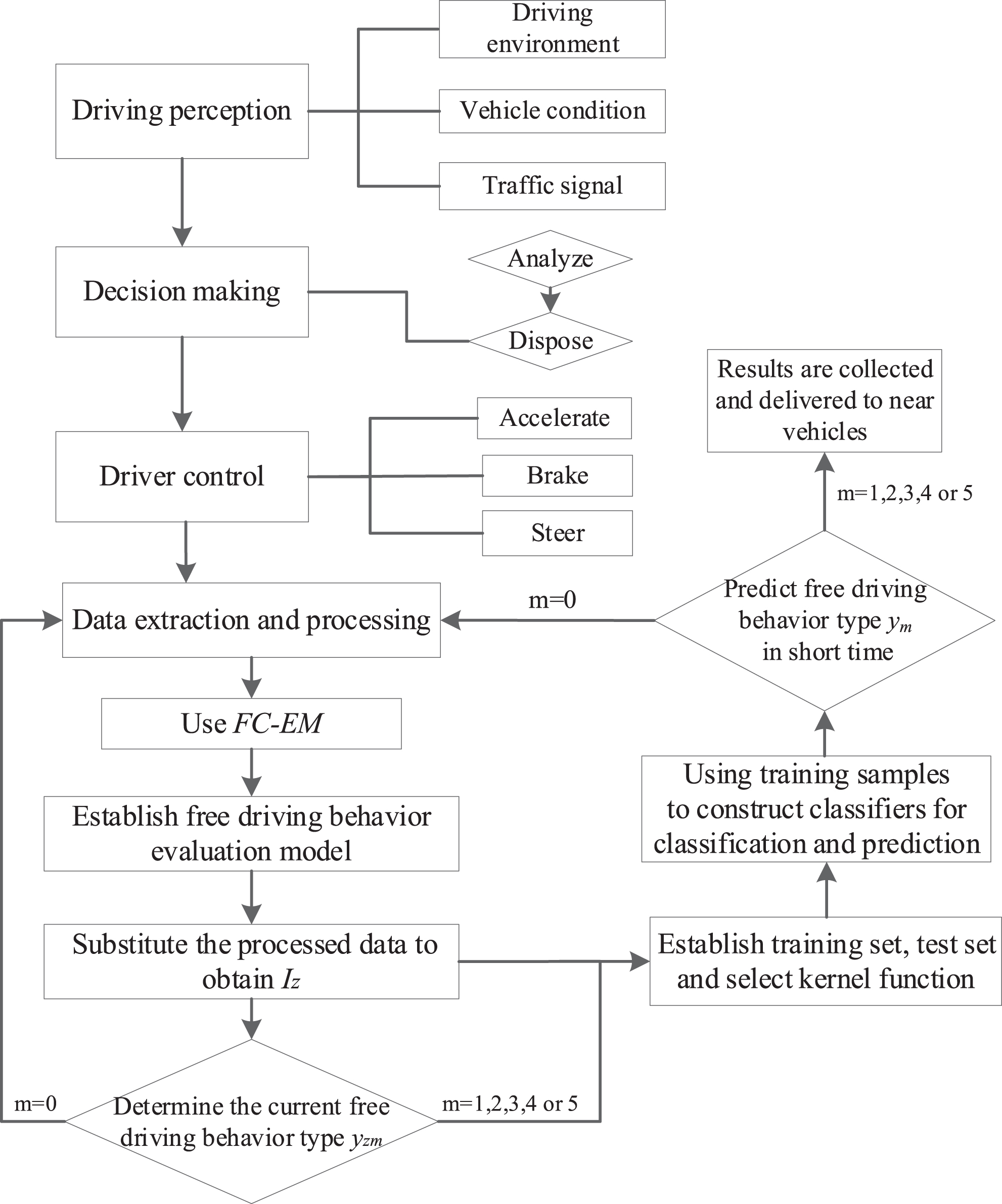
3 Evaluation and prediction of free driving behavior based on FC-SVM

According to the evaluation index system above, the free driving behavior evaluation and prediction based on FC-SVM method is established in Fig. 2. Usually, free driving individuals form cognitive styles that are different from other individuals because they differ in cognitive pattern. Drivers with different cognitive styles have certain differences in free driving types such as driving habits and adaptability to different driving environments. These differences will have an impact on free driving behavior and traffic safety and efficiency.

Fig. 2

Evaluation and prediction model of free driving behavior.

As shown in Fig. 2., the driver usually needs to remain awake in the free driving situation throughout the driving process. It is expressed as a comprehensive, dynamic, accurate and clear perception of the status and attribute information of each relevant element in the driving environment, mainly including the information of the vehicle itself, such as the speed of the vehicle, the condition of the vehicle, the change of the vehicle itself and the surrounding environment. There are also road traffic signals and so on. On this basis, the disorganized information is synthesized, and the meaning of the situation information is analyzed according to different driving purposes. At the same time, the driver operates the steering component for accelerating or braking or steering.

In addition, the system collects a variety of individual control data such as deceleration, acceleration and steering data during driving, and perceive the distance between lane change and other traffic participants and other influencing factors. After that, these obtained multi-category data are processed, for example, the total times the driver drives the throttle to the current position, are converted into the times the driver slams on the accelerator under the current unit mileage and so on. Then, through a series of processes of FC-EM, the current driving behavior score set Iz is obtained, including the current driving behavior safety score I_z1, the driving behavior comfort score I_z2, the driving behavior economic score I_z3, the driving behavior other aspects score I_z4, and total score Iz of the current driving behavior, that is, the z-th group driving behavior score Iz = { I_z1, I_z2, I_z3, I_z4} (z = 1, 2, ⋯). After that, the current driving behavior type y_zm is determined. If m = 1,2,3,4 or 5, (Iz, y_zm) will be input to the SVM, where m represents different free driving behavior type. “m = 1” represents cower driving behavior; “m = 2” represents conservative driving behavior; “m = 3” represents ordinary driving behavior; “m = 4” represents aggressive driving behavior; “m = 5” represents impulsive driving behavior. This is corresponding to the classification in Table 3. Otherwise, the free driving data will continue to be extracted and processed. These data are used to establish training set and test set. RBR kernel function is selected in this paper. Further, training samples are used the OVR(one-versus-rest) classifier is constructed to predict the driving behavior type y_m. Only when m¬ =0 are the results collected and delivered to near vehicles. Through vehicle-to-vehicle information interaction, free driving behavior types of the adjacent vehicles are obtained, and the current vehicle’s driving mode will be changed. Otherwise, m = 0 means the result is invalid, and it is needed to be reacquired.

Table 3

Classification of free driving behavior types

Grading interval	Free driving behavior level (y_m)
[0, 20)	Cower driving behavior (y₁)
20, 40)	Conservative driving behavior (y₂)
40, 60)	Ordinary driving behavior (y₃)
60, 80)	Aggressive driving behavior (y₄)
80, 100]	Impulsive driving behavior (y₅)

3.1 Free driving behavior evaluation model

3.1.1 Fuzzy driving behavior data

In order to eliminate the ambiguity of free driving behavior, fuzzy logic is used to process fuzzy events. Fuzzy logic relies on the concept of membership function, which has advantages of expressing qualitative experience with unknown boundaries, distinguishing fuzzy sets and processing the relationship between them. Besides, it simulates the process of human brain reasoning, makes the execution process regular, and solves the uncertainty caused by “platoon within platoon” [27 –30].

Two-dimensional fuzzy rule:

$\begin{matrix} r_{ij} : IF (ξ is A^{(i)} and ς is L^{(i)}) \\ THEN (y is B^{(i)}) (C_{ij}) \end{matrix}$ (1)

Then the degree of correlation between element A and element B and element C is represented by an (n + 1)-dimensional membership function defined in the multiplication space as follows. $μ_{r_{ij}} (ξ, y) = {\hat{*}}_{μ_{A^{(i)}}} {\hat{*}}_{μ_{L^{(i)}}} {\hat{*}}_{c_{ij}} {\hat{*}}_{μ_{B^{(j)}} (y)}$ (2) $\hat{*}$ is a binary trigonometric paradigm. It is usually represented by a minimum operator or a multiplication operator. When the input of the ij-th fuzzy rules is ξ and ς, the fuzzy set μ_rij (ξ, y) represents the confidence and its output is y. The evaluation model selects two-dimensional fuzzy controller of simulink. The membership functions of error and error variation are triangle and trapezoidal membership function respectively.

After evaluating the driving behavior by FC-EM, a fuzzy vector is obtained indicating the degree where the evaluated object belongs to a plurality of evaluation levels. By defuzzifying the obtained fuzzy vector, the level of the evaluation object can be determined. This paper adopts centroid method, combining the characteristics of various fuzzy operators and research models. The weighting coefficient is u (B_i). The formula for determining the center of gravity element u is as follows: $u = \frac{\sum_{i = 1}^{n} u (B_{i}) \times B_{i}}{\sum_{i = 1}^{n} u (B_{i})}$ (3)

Generally, fuzzy inference in FC-EM has the following four steps: 1) computing membership degree; 2) seeking excitation intensity; 3) applying fuzzy rules; 4) fuzzy clustering reasoning. The result is a fuzzy set, which is defuzzified by the centroid method to obtain the determined value.

In order to comprehensively evaluate free driving behavior, a free driving behavior evaluation model is established to classify multiple factors into vehicle driving safety, driving comfort, fuel economy, and others. Each point under each index uses multi-dimensional fuzzy logic method to transform the multi-factor parameters obtained by data processing into multi-factor evaluation parameters of driving behavior. Each evaluation factor is combined with the complexity of the simulation environment L to build a two-dimensional fuzzy logic evaluation model. The environmental complexity refers to the value of 0 to 1 according to the density ratio of the number of road traffic participants. The target value set corresponding to the environment complexity set is V ={ V₁, V₂, V₃, V₄ }, where each single factor subset in V is: $\begin{matrix} V_{1} = {a_{1}, a_{2}, a_{3}} \\ V_{2} = {b_{1}, b_{2}, b_{3}} \\ V_{3} = {c_{1}, c_{2}, c_{3}} \\ V_{4} = {d_{1}, d_{2}, d_{3}} \end{matrix}$ (4)

In Equation (4), a_i,b_i,c_i and d_i all represent corresponding descriptive evaluation.

Multiple factors to evaluate the driving safety index U₁ include: car-following distance U₁₁; relative distance and speed of vehicles rear to the target lane during lane change U₁₂; number of times the driver runs a red light U₁₃; the number of throttle stamps per mileage during turning U₁₄; the number of times a car slam on the brake per mile during turning U₁₅; total number of lane changes per unit mileage U₁₆.

The six influencing factors for evaluating the driving safety indicators are represented by a set of evaluation factor: U₁ = {U₁₁, U₁₂, U₁₃, U₁₄, U₁₅, U₁₆}. The subset of factors is recorded as: $\begin{matrix} U_{11} = {α_{1}, α_{2}, α_{3}, α_{4}} \\ = {very far, further, near, very poor} \\ U_{12} = {β_{1}, β_{2}, β_{3}} = {further, general, near} \\ U_{13} = {ɛ_{1}, ɛ_{2}} = {seldom, occasionally} \\ U_{14} = {δ_{1}, δ_{2}, δ_{3}} = {seldom, occasionally, often} \\ U_{15} = {χ_{1}, χ_{2}, χ_{3}} = {seldom, occasionally, often} \\ U_{16} = {γ_{1}, γ_{2}, γ_{3}} = {seldom, occasionally, often} \end{matrix}$ (5)

The fuzzy rule corresponding to factor U₁ is: ri₁ : IF (α_iisU_1iANDς_iisL) THEN (a_iisB₁) (Ci₁). Then the inverse fuzzy set gets the exact value v_1i, and the result matrix B₁ is obtained, B₁ ={ v₁₁, v₁₂, v₁₃, v₁₄, v₁₅, v₁₆ }.

Multiple factors to evaluate the driving safety index U₂ include: the number of times a driver steps on the accelerator per unit mileage U₂₁; slam on the brakes per mile U₂₂; distance from the intersection stop line when the driver starts to slow down U_23 . Three influencing factors for evaluating the safety of driving behavior are represented by a set of evaluation factors U₂ ={ U₂₁, U₂₂, U₂₃ }, and the subset of factors is recorded as: $\begin{matrix} U_{21} = {ɛ_{1}, ɛ_{2}, ɛ_{3}} = {seldom, occasionally, often} \\ U_{22} = {δ_{1}, δ_{2}, δ_{3}} = {seldom, occasionally, often} \\ U_{23} = {χ_{1}, χ_{2}, χ_{3}} = {veryfar, general, further} \end{matrix}$ (6)

The fuzzy rule corresponding to the factor U₂ is ri₁ : IF (α_iisU_2iANDς_iisL) THEN (a_iisB₂) (Ci₁). Then the inverse fuzzy set gets the exact value v_2i and the result matrix B₂ = (v₂₁, v₂₂, v₂₃) is obtained. The multi-factors for evaluating the fuel economy index U₃ include judging the driving consumption of the driving vehicle according to the ratio of the duration of the gear to the total driving time, thereby judging the driving habit of the driver.

The five gears used to evaluate fuel economy are expressed in time series U₃ ={ U₃₁, U₃₂, U₃₃, U₃₄, U₃₅ }. The subset of factors U_3i (i = 1, 2, 3, 4, 5) is recorded as: $\begin{matrix} U_{31} = {α_{1}, α_{2}, α_{3}} = {less, general, more} \\ U_{32} = {β_{1}, β_{2}, β_{3}} = {less, general, more} \\ U_{33} = {ɛ_{1}, ɛ_{2}, ɛ_{3}} = {less, general, more} \\ U_{34} = {δ_{1}, δ_{2}, δ_{3}} = {less, general, more} \\ U_{35} = {χ_{1}, χ_{2}, χ_{3}} = {less, general, more} \end{matrix}$ (7)

The fuzzy rule corresponding to the factor U₃ is: ri₁ : IF (α_iisU_3iANDς_iisL) THEN (a_iisB₃) (Ci₁). Then the inverse fuzzy set gets the exact value U_3i, and the result matrix B₃ is obtained: B₃ ={ B₃₁, B₃₂, B₃₃, B₃₄, B₃₅ }.

The other factor is the average driving speed U₄, which is used to evaluate the driver’s driving proficiency. The average driving speed can indirectly reflect whether the driver’s driving behavior is aggressive, and it can be evaluated by U₄ = {α₁, α₂, α₃, α₄} = {veryfast, faster, slower, veryslow}

The fuzzy rule corresponding to the factor U₄ is ri₁ : IF (α_iisU₄ANDς_iisL) THEN (a_iisB₄) (Ci₁). The inverse fuzzy set then gets the exact value B₄.

The evaluation coefficient is combined with the subjective experience judgment method, the expert consultation method and the analytic hierarchy process to determine the weight coefficient subset of each evaluation factor indicator. Each subset weight (primary weight) is A ={ m₁, m₂, m₃, m₄ }. The weights (secondary weights) of the factors in each performance subset A_i (i = 1, 2, 3, 4) are: ${\begin{matrix} A_{1} = {m_{11}, m_{12}, m_{13}, m_{14}, m_{15}, m_{16}} \\ A_{2} = {m_{21}, m_{22}, m_{23}} \\ A_{3} = {m_{31}, m_{32}, m_{33}, m_{34}, m_{35}} \\ A_{4} = 1 \end{matrix}$ (8)

3.1.2 Construct evaluation model

In summary, the FC-EM based on multi-factor free driving behavior evaluation model is established. $I = \sum_{i = 1}^{4} m_{i} B_{i} A_{i}^{'} = \sum_{i = 1}^{4} m_{i} I_{i}$ (9)

In Equation (9), I _i means driving behavior rating on U_i ; I represents free driving behavior comprehensive evaluation score; m_i represents free driving behavior first-order weight indicator weight; B_i means the exact value obtained by anti-blurring of each factor in the free driving behavior evaluation index U; means the secondary weight corresponding to each element in the set B_i.

Among them, the determination process and results of m_i and are as follows. m_i is determined by combining expert consultation with AHP (Analytic Hierarchy Process). It is a widely used method to determine the weight [31, 32]. The FC-EM is based on AHP, and the two complement each other to improve the reliability and effectiveness of evaluation. Therefore, this combination can reduce the subjective dependence of evaluation indicators. Besides, it is difficult for people to accept a qualitative result at the time of determining the weight between various factors at various levels. Therefore, instead of comparing all the factors together, the uniform matrix method uses the relative scale to reduce the difficulty of comparing various factors with different properties to improve the accuracy. First of all, the uniform matrix method proposed by Saaty et al. [33] is used to establish a first-level index pairwise comparison matrix D = [d_ij]_n ×n. The matrix formed by pairwise comparison is called judgment matrix. Comparing element i with element j, d_ij = 1 means that they have the same importance, d_ij = 3 means that i is more important than j, d_ij = 5 means that i is obviously more important than j. d_ij = 2 and d_ij = 4 represent the intermediate values of the above adjacent judgments. The judgment matrix has the following properties: d_ij = 1/d_ji. Combined with literature [34], the judgment matrix in Table 1 can be obtained, as shown in Table 1 below.

Table 1

First-level indicator judgment matrix

Evaluation index	Safety	Comfort	Economy	Other indicator
Safety	1	2	3	4
Comfort	2	1	2	3
Economy	3	1/2	1	2
Others	4	1/3	1/2	1

The geometric mean of the judgment matrix D is $M_{i} = \sqrt[n]{\prod_{j = 1}^{n} d_{ij}}, i = 1, 2, \dots, 4; n = 4$ .

Calculate the n-th root of M_i, $\bar{w_{i}} = \sqrt[n]{M_{i}}, n = 4$ . Normalize the processing of column vectors $\bar{w} = (\bar{w_{1}}, \bar{w_{2}}, \dots, \bar{w_{n}})$ and get weights: $\begin{matrix} A & = [m_{1}, m_{2}, m_{3}, m_{4}] \\ = [0.467, 0.278, 0.160, 0.095] . \end{matrix}$

Secondly, calculate the maximum eigenvalue of the judgment matrix:λ_max = 4.03.

Consistency indicator CR is $CR = \frac{CI}{RI} = (\frac{4.03 - 4}{4 - 1}) / 0.89 = 0.011 < 0.1$

Therefore, the judgment matrix consistency test is satisfied, and the feature vector is recognized, and the first-order weight matrix of the driving behavior evaluation method is obtained, as shown in Table 2.

Table 2

Weights of different indicators

The weight grade

First-level indicator weight

Primary indicator

U₁

U₂

U₃

U₄

Weight

0.467

0.278

0.160

0.095

The weight grade

Secondary indicator weight

Indicator 1

U ₁₁

U ₁₂

U ₁₃

U ₁₄

U ₁₅

U ₁₆

Weight

0.25

0.20

0.15

0.05

0.10

Indicator 2

U ₂₁

U ₂₂

U ₂₃

Weight

0.35

0.30

Indicator 3

U ₃₁

U ₃₂

U ₃₃

U ₃₄

U ₃₅

Weight

0.30

0.25

0.20

0.15

0.10

${A^{'}}_{i}$ is determined by combining expert inquiry method with subjective experience judgment method. Among them, other indicators have no secondary weights, and the weights of indicators of safety, comfort, and economy are also shown in Table 2. Each parameter has been explained in the Fig. 1 above.

According to the literature [35, 36], the general driving behavior can be divided into a cowering type, a conservative type, an ordinary type, an aggressive type, and an impulsive type. The free driver’s driving behavior evaluation score that can be obtained through Equation (9), and accordingly the free driving behavior type can be obtained by referring to Table 3 below. Among them, the cowering type indicates that the traffic rules are strictly observed during the free driving process of the vehicle, and the other vehicles are carefully driven while the driver is nervous during driving. The conservative type indicates that the vehicle is cautious in obeying the traffic rules without affecting the normal driving of other and the general driving speed is not high. The ordinary type means safe and smooth driving at normal speed without violating the traffic rules. Aggressive type means occasionally violating the traffic rules and driving during the free driving process, slightly affecting the normal driving of others. Impulsive type indicates that the traffic rules are often violated, hindering the normal driving of others, and the driving speed is too high to guarantee the driving safety.

3.2 Free Driving behavior prediction model

The SVM is based on the principle of structural risk minimization and the dimension theory in statistics. Based on the limited sample information, the SVM seeks the best compromise between the complexity of the model and the learning ability, which can be applied to classification problems and can have unique advantages in solving small sample, nonlinear and high-dimensional pattern recognition [37]. In FC-SVM, SVM reduces the influence of subjective factors on the weight of FC. The free driving behavior score and free driving behavior evaluation type of FC-EM constitute the input of SVM (I_z, y_m_Z). I_z is the free driving behavior score after the z-th group fuzzy comprehensive analysis, and y_mz is the z-group driving behavior evaluation type (z = 1, 2, ⋯; m = 1, 2, 3, 4, 5).

In the case of linear separability, the SVM is proposed to obtain the optimal classification plane. For a linearly separable sample set, there is a hyperplane w^Tx_i + b = 0, by determining the positive and negative of g (x_i) = w^Tx_i + b to confirm which class x_i in the sample set belongs to. w is the normal vector of the hyperplane, T stands for transpose, and b is the offset, which determines the distance of the hyperplane from the origin. When some sample points in the sample are linearly inseparable, the relaxation variable ξ_i (ξ_i≥0, i = 1, 2, ⋯, n) is introduced, but not all sample points have slack variables. ξ_i does just apply to outliers in the sample, in which case the hyperplane must meet the conditions: $y_{i} (w^{T} x_{i} + b) ⩾ 1 - ξ_{i}$ (10)

When ξ_i <1, the sample points can still be correctly classified. When ξ_i≥1, the classification surface cannot classify the samples correctly, so the following function is introduced. $φ (w, ξ) = \frac{1}{2} w^{T} w + C \sum_{i = 1}^{n} ξ_{i}$ (11)

Among them, C is a penalty factor, which indicates the trade-off between good generalization ability and minimum training error. At this time, SVM is realized by quadratic programming as follows [38, 39]. ${\begin{matrix} max \sum_{i = 1}^{n} a_{i} - \frac{1}{2} \sum_{i = 1}^{n} \sum_{j = 1}^{n} a_{i} a_{j} y_{i} y_{j} (x_{i}^{T} x_{j}) \\ s . t . a_{i} ⩾ 0, i = 1, 2, \dots, n \\ \sum_{i = 1}^{n} a_{i} y_{i} = 0 \end{matrix}$ (12)

Substituting the kernel function K (x_i, x_j) for $x_{i}^{T} x_{j}$ is equivalent to mapping the original sample to a high-dimensional space. This process makes the linear indivisible problem linearly separable, and finally obtains the classification function: $f (x) = sgn (\sum_{i = 1}^{n} a_{i} y_{i} K (x_{i} \cdot x) + b)$ (13) where a_i is the lagrange multiplier, b is the threshold, and K(x_i, x_j) is the kernel function. Commonly used kernel functions are polynomial kernel function, RBF kernel function and Sigmoid kernel function.

There are currently two ways for SVM linear classifiers to solve multi-classification problems: (1) One-versus-one (OVO SVMs), which is used to design an SVM between any two types of samples, so samples of k categories need to design k(k-1)/2 SVMs. (2) One-versus-rest (OVR SVMs) training classifies samples of one category into one class in turn, and other remaining (k-1) class samples are classified into another class. When classified, the unknown sample is classified as the one with the largest classification function value. Comparing these two methods, OVO SVMs are computationally intensive and complex in structure, and are used less in practical applications. Therefore, OVR SVMs are used in the classification prediction of driving behavior types.

According to the given training set where T = { (x₁, y₁) , ⋯ , (x_L, y_L) } ∈ (X × Y) ^L, x_i ∈ X = Rⁿ, y_i∈ Y = { 1, 2 ⋯ , M } (i = 1, 2 ⋯ L), a decision function is looked for.

To get a multi-class classifier, a series of two-class classifiers is needed to be constructed. Firstly, a certain type of free driving behavior is taken as a category, and the remaining free driving behavior types are used as a class to construct a classifier to classify driving behaviors. In this way, multiple classifiers are designed to classify and predict driving behavior types. Next, it is presumed to judge the attribution of a certain input x. The specific description is as follows.

Under the training set of Equation (14), the following operations are performed like that the j class is denoted as “1”, and the remaining (M-1) classes are denoted as “–1”, and decision function is found by SVM Equation (12): $f^{j} (x) = sgn (g^{j} (x))$ (14) where gj(x) determines that input x belongs to j-th category, and j is the largest value between 1 and M.

4 Experiment

4.1 Experimental description

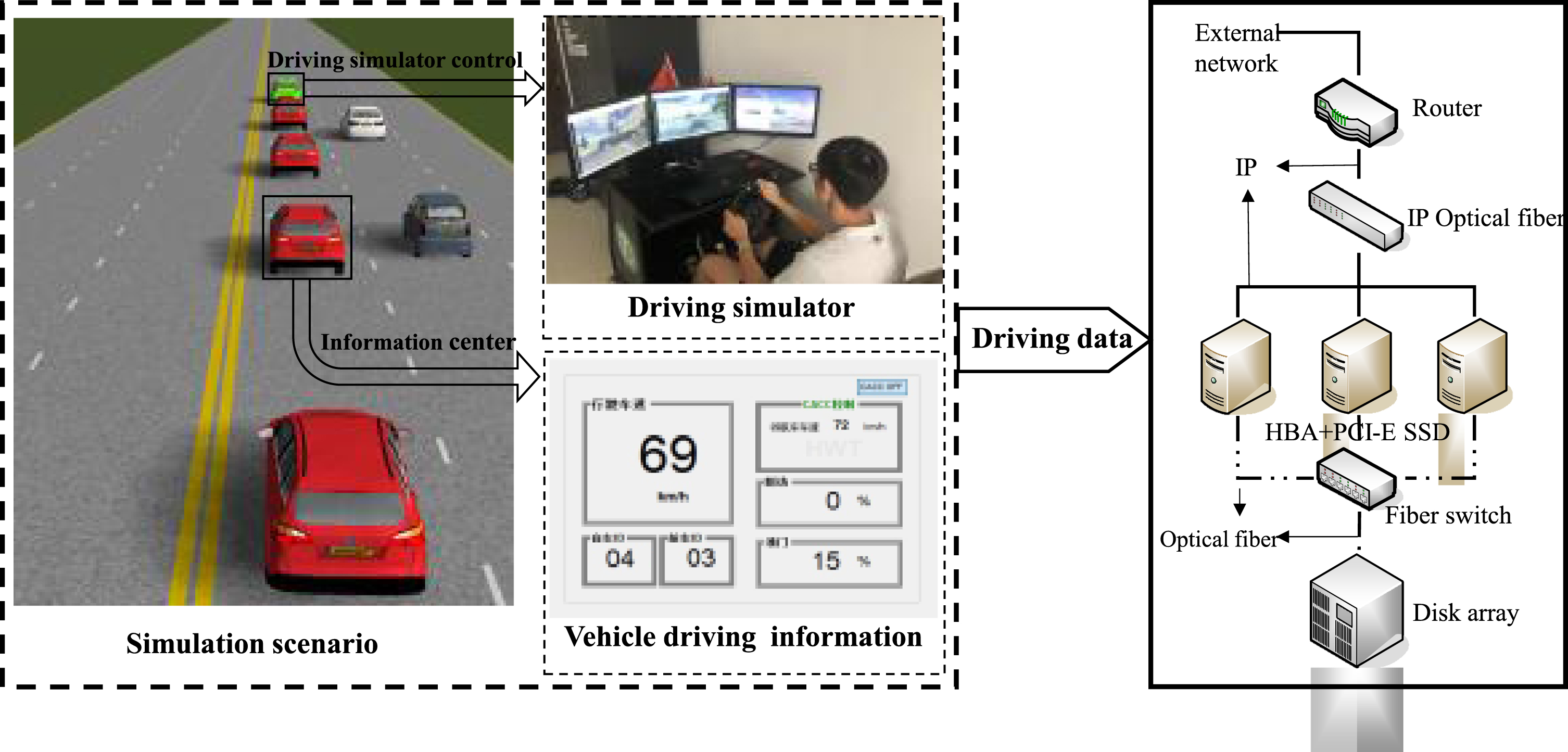
Prescan and Matlab/Simulink joint simulation is used to build the simulation platform shown in Fig. 3. Through Prescan, the driving road of the typical 3 km section of Zhihui Avenue in Jingkou District of Zhenjiang was built to simulate the free driving situation of the road in real scene, and the road ratio was 1:1. Using Sketchup to build a driving participation scene around the road, the driving environment simulates the real environment, avoiding large errors in the simulation results due to changes in the driving environment. Various vehicles, traffic lights, marking rods, sensors and other modules are added to the traffic scene. Although the experimental scenario was designed to be as close to the real world as possible, there are still some differences between them. Fortunately, some differences in the external environment do not have much impact on the vehicle, driving simulation experiments focus on the current road vehicles and the driver himself. The driving simulator controls the vehicle Audi_A8_1, and the driver manipulates the simulator to simulate the real free driving scene.

Fig. 3

Prescan simulation platform.

In the typical driving simulation scenario built by Prescan, the driver simulates the real driving vehicle, and collects the throttle and brake pedal opening, steering wheel angle and gear position of the vehicle. At the same time, the relative distance between the simulated vehicle and the front or rear vehicles in the traffic environment is collected. Besides, the vehicle speed and intersection traffic light status are collected. The parameters that can be collected by the vehicle are converted into parameters related to driving behavior by Matlab/Simulink. Because there are some differences between the driving simulator simulation and real vehicle test to some degree, experiments done in the following are all based on the improved driving platform, which can improve the fidelity of simulators and be closer to real vehicle.

We used accumulated mileage to distinguish the driving experience of participants in this study by reference to two studies [40, 41]. Accumulated mileage is the total number of driving mileage by the data of statistics. The drivers with accumulated mileage less than 3000 km are novices. The drivers with accumulated mileage between 3000 km and 100,000 km are medium experienced. The drivers with accumulated mileage more than 100,000 km are experienced. The participants that took part in our experiments are divided into medium experienced drivers and experienced drivers, as shown in supplementary Table 4. Specific experiments (Experiment 1–5) are described in the following sections.

Table 4

Attributes of the participants

Experiments	Participant	Average age	Driving experience
			Medium	Experienced
Experiment 1	A male driver	30	0	1
Experiment 2	A male driver	30	0	1
Experiment 3	10 drivers (5 males and 5 females)	31.2	5	5
Experiment 4	20 drivers (10 males and 10 females)	32.3	10	10
Experiment 5	5 drivers (different free behavior types)	29.9	2	3

4.2 Evaluation experiment

Free driving behavior evaluation adopts three control strategies. The three control strategies are as follows: 1) Driving behavior score was obtained by weighted synthesis method (WE-SY); 2) Analytic hierarchy process (AHP) was used to obtain driving behavior score; 3) The Matlab fuzzy toolbox was used to establish the corresponding fuzzy rules and set the basic parameters of the fuzzy module of Simulink. The driving behavior evaluation model based on established FC-EM above was used to obtain the driving behavior evaluation score.

Experiment 1: Simulation test: A male driver aged 30 that are experienced was selected to participate in the simulation experiment of driving behavior based on Prescan. In the built simulation scenario, the driver performs a single driving simulation, and Prescan collects simulation data in real time to obtain different driving behavior scores under different environmental complexity (different environmental complexity is achieved by adding the number of surrounding vehicles and pedestrians), as shown in Fig. 4. “L₁ = 0.25” and “L₂ = 0.5” represent respectively lower environment complexity and higher environment complexity. The reason why we choose the two kinds of case instead of other kinds is that the road traffic will become congested under higher environment complexity than 0.5. This experiment aims to evaluate the driving behavior type, while the driver will form his own unique free driving behavior type during the long-term driving process [8], so our evaluation experiment set can derive the driver’s accurate free driving behavior type in the two kinds of cases.

Fig. 4

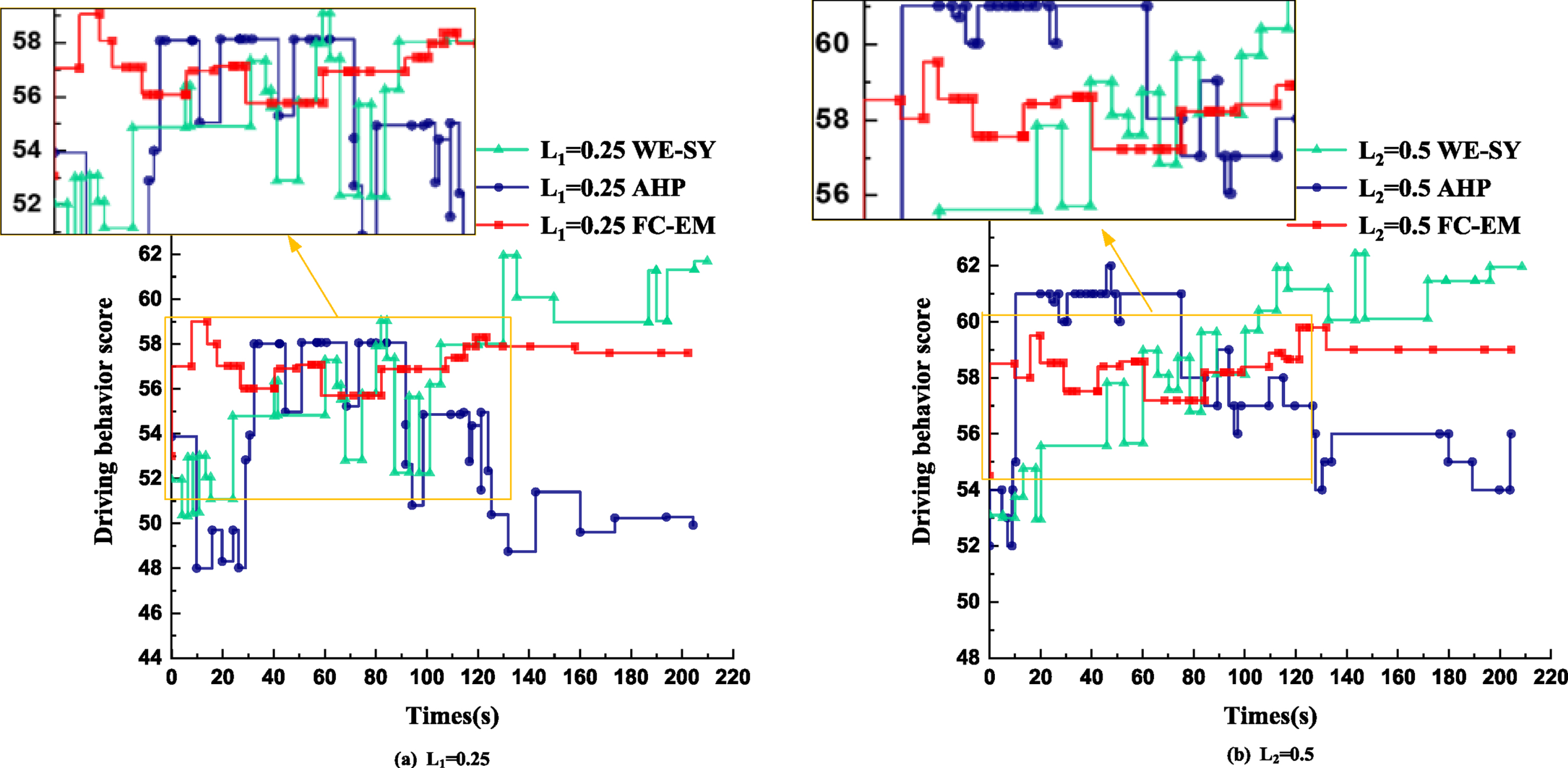
Comparison of the same driver’s single driving score.

Available from Fig. 4: (1) When L₁ = 0.25, the driving score curve obtained by FC-EM tends to be fixed after short-time simulation, while the simulations of the other methods are still large at the end of simulation. L₂ = 0.5 is also like this. (2) Whether L₁ = 0.25 or L₂ = 0.5, using the FC-EM to obtain the driving behavior score, due to the environmental complexity in the model, the scoring curve fluctuates greatly at the beginning of the simulation. With the increase of the simulation time, the evaluation can be performed within a few minutes without sudden traffic conditions. A stable driving behavior score can be obtained, thereby obtaining a stable type of free driving behavior.

Experiment 2: Under different environmental complexity, the same driver mentioned in Experiment 1 performs 20 simulations for the three control strategies on the same simulation scenario. The reason for choosing the same driver is keeping other influencing factors unchanged except his own condition. The final result is shown in Fig. 5.

Fig. 5

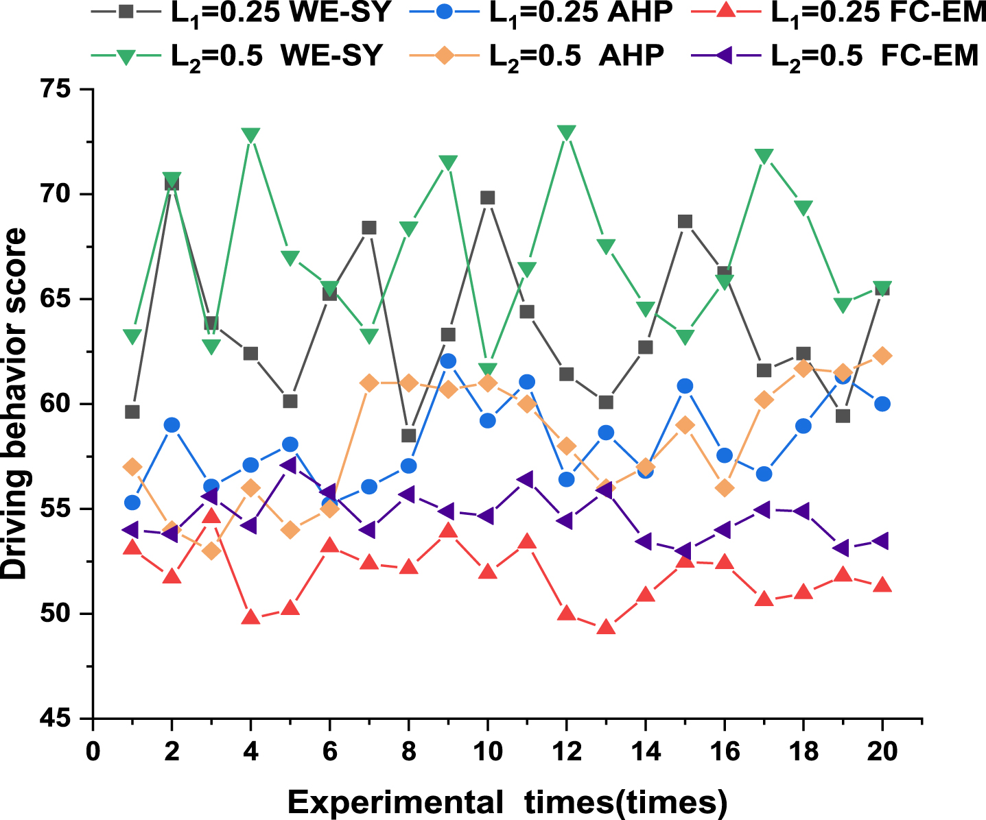
Comparison of the same driver’s multiple driving behavior scores.

Variance (VA) is used to measure the discreteness of driving behavior evaluation results, as shown in Equation (15). Besides, Standard Deviation (SD) [42] is used as an analysis index for driving behavior evaluation, as shown in Equation (16). $VA = 1 / N \sum_{i = 1}^{N} (x_{i} - \bar{u})^{2}$ (15) $SD = \sqrt{1 / N \sum_{i = 1}^{N} (x_{i} - \bar{u})^{2}}$ (16)

$\bar{u}$ represents the average value of the data. The calculated results are shown in Fig. 6 (a) and (b) respectively, which is used to measure the dispersion degree of the driving score value itself. The smaller the SD and VA, the better the stability.

Fig. 6

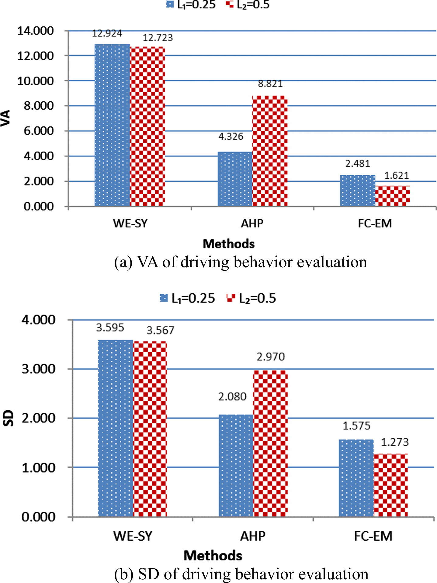
Analysis of driving behavior scores.

Available from Figs. 5 6:

Under L₁ = 0.25 or L₂ = 0.5, the driving behavior scores using FC-EM are lower than the other methods’ scores, and the FC-EM driving behavior score curve is smaller than other methods, and the analysis index SD and VA are also small, which proves that FC-EM has good stability.

When the environmental complexity increases to L₂ = 0.5, the SD value of FC-EM is only 1.273, while the SD value of AHP is more than twice as much as it, and the SD value of WE-SY is nearly three times that. Overall, it proves that the evaluation model using FC-EM is more adaptable to the environment.

Combined with Table 3, under L₁ = 0.25 or L₂ = 0.5, the evaluation results using FC-EM are all ordinary driving behaviors, while the evaluation results of others fluctuate between aggressive and ordinary driving behaviors, and these results are not stable enough.

Based on the Experiment 1 and Experiment 2 comprehensively, the evaluation of driving behavior based on FC-EM can more specifically evaluate the driver’s personalized driving.

4.3 Prediction experiment

Experiment 3: Select 10 drivers (5 males and 5 females) consisting of 5 medium experienced drivers and 5 experienced drivers, and each driver alternately simulates 20 complete driving processes in the simulated scene (selecting L₁ = 0.25). After using FC-EM, the final 200 groups of driving behavior scores and the respective driving type m are obtained, where number Z is from 1 to 200 and the range of input IZ is [0,100]. 120 groups of the sample data (1–120) are shown in Table 5, of which each parameter has been explained in section 3, and the rest 80 groups (121–200) are used as test set data to predict the free driving behavior.

Table 5
120 groups of sample data table

Number Z Input I_z = I_z1, I_z2, I_z3, I_z4 Output y_m

I_Z1 I_Z2 I_Z3 I_Z4 type m

1 45.2 58.3 49.3 50 3

2 46.3 54.4 48.4 50 3

3 65.8 78.3 69.7 60 4

4 68.2 70.3 63.1 60 4

5 50.3 62.2 54.1 60 3

6 51.1 63.1 54.3 60 3

7 45.4 58.6 49.6 50 3

8 46.8 58.7 48.9 50 3

9 87.5 92.1 85.2 80 5

10 88.4 93.9 83.3 80 5

⋮ ⋮ ⋮ ⋮ ⋮ ⋮

120 51.2 63.3 54.4 60 3

Number Z	Input I_z = I_z1, I_z2, I_z3, I_z4	Output y_m
1	45.2	58.3	49.3	50	3
2	46.3	54.4	48.4	50	3
3	65.8	78.3	69.7	60	4
4	68.2	70.3	63.1	60	4
5	50.3	62.2	54.1	60	3
6	51.1	63.1	54.3	60	3
7	45.4	58.6	49.6	50	3
8	46.8	58.7	48.9	50	3
9	87.5	92.1	85.2	80	5
10	88.4	93.9	83.3	80	5
⋮	⋮	⋮	⋮	⋮	⋮
120	51.2	63.3	54.4	60	3

There are many types of kernel functions, such as Linear kernel, Polynomial kernel, Sigmoid kernel and RBF kernel. Because the RBF kernel can map the sample to a higher dimensional space, it can handle the example when the relationship between class labels and features is non-linear. In addition, compared with Polynomial Kernel, RBF kernel has the advantage of fewer parameters, so RBF kernel has lower complexity of model selection. Also, it is important to note that the sigmoid kernel is incorrect for some parameters, such as no inner product of two vectors. Therefore, in the FC-SVM method, the classification experiments are carried out by selecting RBF kernel function as the optimal kernel function. The training and prediction of the model are carried out by using the SVM toolbox of Matlab.

After using the FC-SVM method to predict the type of free driving behavior, the following evaluation indicators can be used for analysis [43, 44]:

Accuracy rate of class m driving behavior (P_m): $P_{m} = \frac{l_{m}}{M_{m}}$ (17)

M_m is the number of the m-th class output by the classification system, and l_m is the correct classification number in M_m.

Recall rate of class m driving behavior (R_m): $R_{m} = \frac{l_{m}}{N_{m}}$ (18)

N_m is the number of all the test data belonging to the m-th class, and l_m is the number with the correct result of the m-class output through the classification system.

Comprehensive classification rate of class m driving behavior (F1 _m): $F 1_{m} = \frac{2 P_{m} R_{m}}{P_{m} + R_{m}}$ (19)

P_m is the accuracy of the m-th class, and R_m is the recall rate of the m-th class.

Macro average precision (MacropP) $M ac roP = \frac{1}{w} \sum_{t = 1}^{w} P_{t}$ (20)

P_t is the accuracy of the t-th class and w is the total number of all categories. After predicting the free driving behavior type by Decision Tree (ID3), Random Forest and SVM, the Equation (17)–(20) are used to analyze, and the evaluation results are shown in Table 6.

Table 6

Evaluation of prediction results

Prediction methods	Evaluation index	Free driving behavior type (m)
		m = 3	m = 4	m = 5
Decision Tree(ID3)	P _m	80.0%	81.2%	79.7%
	R _m	85.6%	86.7%	83.6%
	F1_m	82.7%	83.9%	81.6%
	M crop	80.3%
Random Forest	P _m	83.8%	86.4%	84.7%
	R _m	90.0%	93.5%	89.2%
	F1_m	86.7%	89.8%	86.9%
	M crop	85.0%
SVM	P _m	88.7%	91.2%	87.7%
	R _m	92.3%	94.5%	93.2%
	F1_m	88.3%	90.2%	89.0%
	M crop	89.2%

Among them, MacropP is up to 89.2%, and the comprehensive classification rate F1 _m of each category is not less than 88.3% for using SVM. Obviously, compared with other methods [45, 46], prediction using SVM has highest MacroP, which verifies the accuracy of FC-SVM classification prediction based on SVM. Besides, when m = 4 (that is aggressive driving behavior), its P_m, R_m and F1 _m are all highest. It can be seen that the type of aggressive driving is more distinct from other types.

Experiment 4: In order to further verify the environmental adaptability of the prediction method, 20 drivers consisting of 10 medium experienced drivers and 10 experienced drivers were selected (10 males and 10 females), each of which simulates 15 complete free driving processes on the L₁ = 0.25 and L₂ = 0.5 simulation scenes, respectively, as Group1. Among them, the ratio of test set to verification set is 3:2. After predicting the free driving behavior type by FC-SVM method, different types of P_m, R_m and Fl_m are calculated respectively. One week apart, the previous 20 drivers performed the same experiment and the result was recorded as Group2. Similarly, Group3 to Group10 is generated accordingly, and the statistical results of the three types of evaluation indicators on prediction are shown in Fig. 7. For example, every data point in Fig. 7(a) represents P_m value corresponding to m value under the current experiment ID, where m represents free driving behavior type and P_m is accuracy rate of class m.

Fig. 7

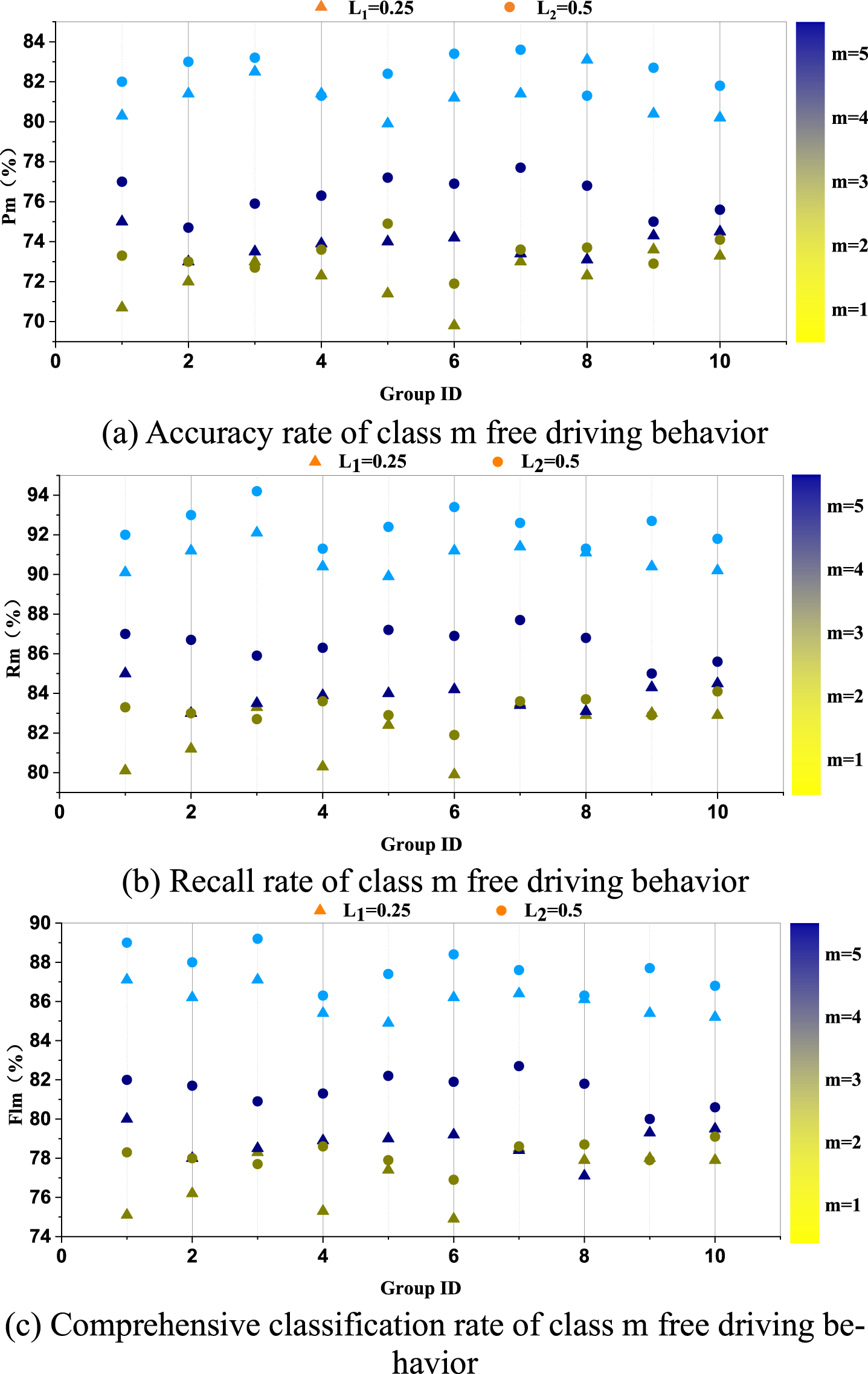
Statistical results of different evaluation indexes.

In Fig. 7, the free driving behaviors of the 20 drivers are concentrated in m = 3, m = 4, and m = 5, and the results of the evaluation of free driving behavior are relatively stable. In the same Group ID experiment, when the environment is more complicated, the larger the corresponding P_m, R_m and F_lm, the more accurate the FC-SVM classification prediction, and the stronger the environmental adaptability of the prediction method. When the driver’s driving type is certain, the fluctuations of different evaluation indexes are not large compared with different groups. Especially when m = 4 (that is aggressive driving behavior), the fluctuations of P_m, R_m and F_lm are smaller and more stable.

4.4 Application experiment

Experiment 5: The urban expressway simulation scenario is constructed as Fig. 8(a). There are two types of vehicles. One is manual vehicle (MV), and the other is connected automatic vehicle (CV). Among these vehicles, the MV is controlled by driving simulator considered as free driving behavior, the other various CVs are added on the way. Five people representing different free behavior types are selected to manipulate simulator in planned path. Each person completed a driving simulation along a planned route in Fig. 8(a) and Table 7. Specific simulation scenario is described as Fig. 8(b). The vehicle exchanges information with outside world through V2X which is key technologies for intelligent transportation systems.

Fig. 8

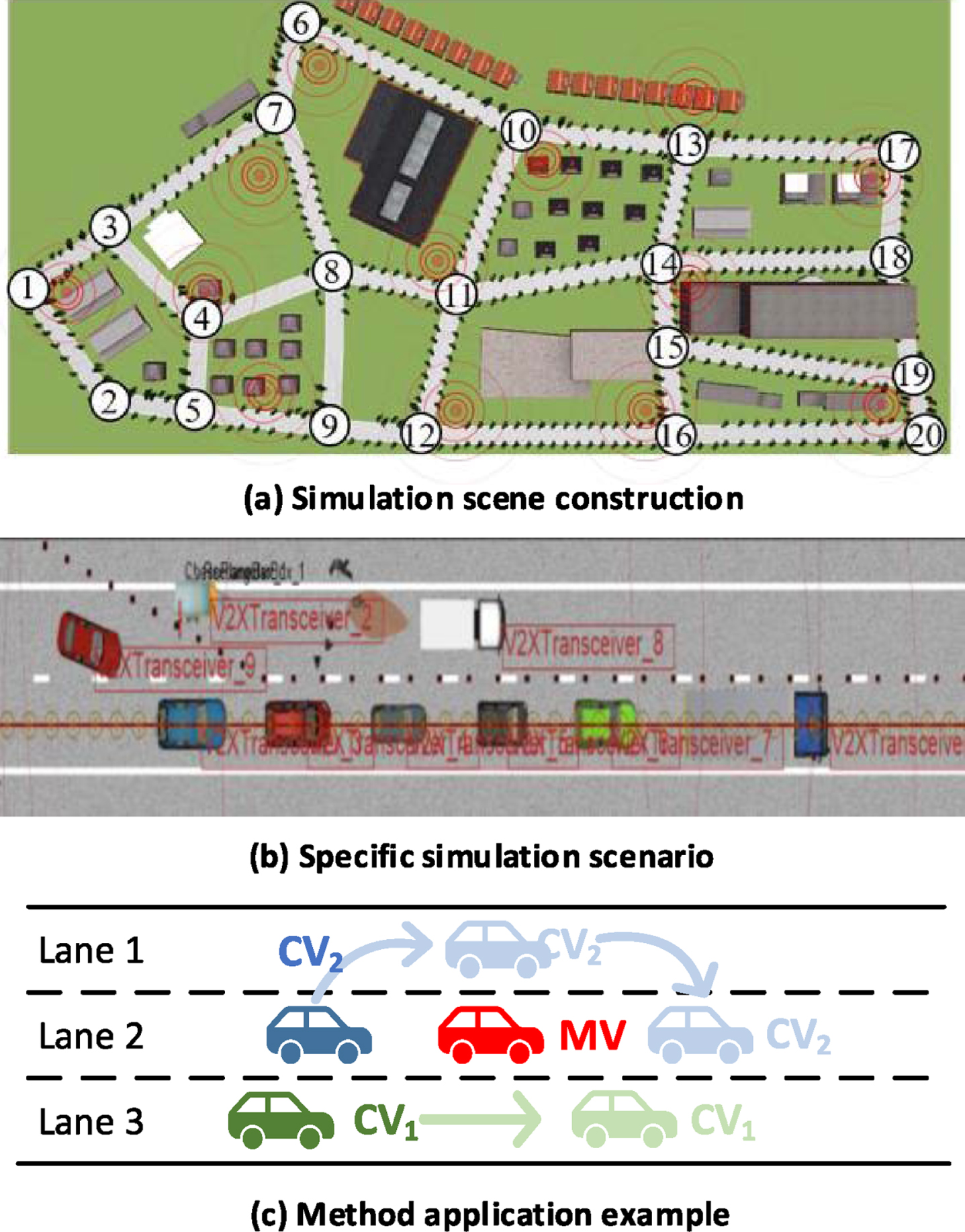
Method applied in an experiment scenario.

Table 7

Results of FC-SVM application

Current driver type(y_m)	FC-SVM applied	Planned path	Distance (m)	Relative minimum time headway ratio (%)	Relative to the total time taken (%)
m = 1	1⟶3⟶4⟶8	1⟶3⟶4⟶8⟶11⟶10⟶13⟶14	3916	+0.5	–5.26
m = 2	11⟶14	1⟶3⟶4⟶8⟶11⟶14	3025	+1.1	–5.12
m = 3	11⟶14	1⟶3⟶4⟶8⟶11⟶14	3025	+1.6	–5.14
m = 4	11⟶14	1⟶3⟶4⟶8⟶11⟶14	3025	+3.2	–6.27
m = 5	1⟶3⟶4⟶8	1⟶3⟶4⟶8⟶11⟶10⟶13⟶14	3916	+2.1	–6.06

Accordingly, one kind of the method’s application examples is depicted in Fig. 8(c). When current MV free driving behavior type result is cower(m = 1) after applying FC-SVM method, nearby cars obtaining this behavior information will change current driving pattern. For example, CV₂ following MV will choose to overtake it on the left. Meanwhile, the back right CV₁ will speed up on the right. Relative minimum time headway ratio and relative to the time taken are used to separately evaluate the application’s safety and efficiency. Time headway (TH) represents the time difference between the front ends of two vehicles passing through the same location. Relative minimum time headway ratio means the relative rate of the minimal TH after using this method in strongly following state. These results are shown in Table 7. Relative minimum time headway ratio is used to judge road safety, and relative to the total time is used to evaluate road efficiency. It is obvious to see that using this method makes minimum time headway increase and makes total driving time decrease. Whatever type the current driver is, the road safety and efficiency are improved. For example, comparing m = 1 with m = 5, the planned path and distance are the same, but relative minimum time headway ratio of m = 5 is larger and decreased time is smaller. The reason for this is that after applying FC-SVM surrounding vehicles stay away from impulsive driving behavior(m = 5) and this kind of impulsive driver can pass fast. Besides, when m = 4 (that is aggressive free driving behavior), the application effect of the method is the most obvious, compared with other free driving behavior types, which is consistent with the discovery mentioned above. The mixed traffic flow composed of aggressive driver has a higher traffic efficiency in basic sections.

5 Conclusion

This paper proposes a free driving behavior evaluation and prediction method based on FC-SVM, which solves the problems that current driving behavior evaluation model has single factor, and the environmental adaptability is insufficient, and the behavior type is difficult to predict accurately. More importantly, this makes up for some deficiencies of existing studies.

In the FC-SVM method, the established free driving behavior evaluation model considers both the influence of the individual behavior and the influence of environmental factors. It has excellent performance when dealing with the classification and prediction of driving behavior types. Therefore, when the environment is more complicated, the FC-SVM driving behavior evaluation result SD is only 1.273, which is lower than the other methods. For the prediction of future driver behavior types, the macro average accuracy is as high as 89.2%, and the comprehensive classification rate of each category is not less than 88.3%. Multiple sets of experiments results show that the environment is more complicated, the larger the corresponding P_m, R_m and F_lm, the more accurate the FC-SVM classification prediction and the stronger the environmental adaptability. It is also interesting to find that aggressive driving can be more distinct from other types. Moreover, the mixed traffic flow composed of aggressive driver has a higher traffic efficiency in basic sections, which can be applied to further driving behavior research.

Nowadays, there are many studies on specific driving phenomena and specific driving populations, but there are few studies on free driving behavior type and evaluation and prediction of driving behavior models. It is necessary for these models to be further supplemented in the future. In the mixed traffic flow under the Internet of Vehicles, using information interaction to judge the free driving behavior of the neighboring vehicle drivers and switch the driving mode is beneficial to improving the stability and safety of the mixed traffic flow, and alleviating traffic congestion.

Footnotes

Acknowledgments

The authors would like to thank the anonymous reviewers for their critical and constructive comments and suggestions. The authors are also thankful to National Key Research and Development Plan(2018YFB1600500) and Major Natural Science Research Project of Colleges and Universities in Jiangsu Province (18KJA580002).

References

Useche

S.A.

, Gomez Ortiz

and Cendales

B.E.

, Stress-related psychosocial factors at work, fatigue, and risky driving behavior in bus rapid transport (BRT) drivers, Accident Analysis and Prevention 104 (2017), 106–114.

Aghamolaei

, Ghanbarnejad

, Tajvar

, Asadiyan

and Ashoogh

, Prediction of driving behaviors base on Theory Planned Behavior (TPB) model in truck drivers, Life Science Journal 10 (2013), 80–84.

Verschuur

W.L.G.

and Hurts

, Modeling safe and unsafe driving behaviour, Accident Analysis & Prevention 40(2) (2008), 644–656.

Oman

L.D.

, et al., Multi-model assessment of the factors driving stratospheric ozone evolution over the 21st century, Journal of Geophysical Research D: Atmospheres 115(24) (2010), 9–12.

P.-f.

, Research on driving behavior characterization indicators and analysis methods, Ph.D. Dissertation, Jilin University, (2010).

Yang

P.-f.

, Research on Operational Driver Safety Assessment Method, Ph.D. Dissertation, Chang’an University, (2013).

, Multi-attribute evaluation method and application research of driving behavior safety, Ph.D. Dissertation, Jilin University, (2016).

Zhao

C.Y.

, et al., Driving rule extraction based on cognitive behavior analysis, Journal of Central South University 27(1) (2020), 164–179.

Chai

, et al., Driver Fatigue Classification With Independent Component by Entropy Rate Bound Minimization Analysis in an EEG-Based System, IEEE Journal of Biomedical & Health Informatics 21(3) (2017), 715–724.

10.

, Woo

and Tamura

, Driver classification in vehicle following behavior by using dynamic potential field method, in Intelligent Transportation Systems (ITSC), IEEE 20th International Conference on. IEEE (2017), 1–6.

11.

, Drivers Classification Based on the Driver Lane Change Behavior Parameters, International Journal of Material & Mechanical 5 (2016), 53.

12.

Ayres

L.L. T

and T.D., Passenger-side rear-view mirrors: driver behavior and safety, International journal of industrial ergonomics 35(2) (2005), 157–162.

13.

Mao

, Lane change warning Method considering driving style Ph.D. Dissertation, Chang’an University, Xi’an, (2012).

14.

Yang

Q.I.

and Koutsopoulos

H.N.

, A Microscopic Traffic Simulator for evaluation of dynamic traffic management systems, Transportation Research Part C 4(3) (1996), 113–129.

15.

Wang

, Zhang

, Liu

, Yunyun

, Wang

and Wang

, The drivers’ lane selection model basedonmixed fuzzy many-person multi-objective non-cooperative game, Journal of Intelligent & Fuzzy Systems 32(6) (2017), 4235–4246.

16.

Daamen , et al., Game theoretic approach for predictive lane-changing and car-following control, Transportation Research Part C 58 (2015), 73–92.

17.

Yang

, Xu

, Lian

, Bin

and Ma

, Multiple flood vulnerability assessment approach based on fuzzy comprehensive evaluation method and coordinated development degree model, Journal of Environmental Management 213 (2018), 440–450.

18.

Xue

, Ding

, Zhang

, Wu

and Wang

, A fuzzy system of operation safety assessment using multi-model linkage and multi-stage collaboration for in-wheel motor, IEEE Transactions on Fuzzy Systems PP(99) (2021), 1–1.

19.

Chen

S.H.

and Gao

C.H.

, Linear Priors Mined and Integrated for Transparency of Blast Furnace Black-Box SVM Model, IEEE Transactions on Industrial Informatics 16(6) (2020), 3862–3870.

20.

Liang

X.W.

, Jiang

A.P.

, Li

, Xue

Y.Y.

and Wang

G.T.

, LR-SMOTE - An improved unbalanced data set oversampling based on K-means and SVM, Knowledge-Based Systems 196 (2020), 10.

21.

Xiong

, Chen

, Liang

, Cai

and Chen

, A Study on the Driving Behavior Prediction of Dangerous Lane Change, Automotive Engineering 39(9) (2017), 1040–1046.

22.

Lin

and Wang

, Fuzzy Support Vector Machines, IEEE Transactions on Neural Networks 13(2) (2002), 464–471.

23.

Xue

Z.X.

, Zhang

R.X.

, Qin

C.D.

and Zeng

X.Q.

, An adaptive twin support vector regression machine based on rough and fuzzy set theories, Neural Computing & Applications 32(9) (2020), 4709–4732.

24.

Martinelli

, Mercaldo

, Orlando

, Nardone

, Santone

and Sangaiah

A.K.

, Human behavior characterization for driving style recognition in vehicle system, Computers & Electrical Engineering 83(1) (2020), 1–16.

25.

Yao

, et al., Vehicle Fuel Consumption Prediction Method Based on Driving Behavior Data Collected from Smartphones, Journal of Advanced Transportation 2020 (2020), 1–11.

26.

Hai-qing

, Research on vehicle safety comprehensive evaluation based on driver cognition, M.D. Thesis, Beijing Forestry University, (2006).

27.

Kabir

and Papadopoulos

, A review of applications of fuzzy sets to safety and reliability engineering, International Journal of Approximate Reasoning 100(9) (2018), 29–55.

28.

Arqub

O.A.

, Al-Smadi

, Momani

and Hayat

, Application of reproducing kernel algorithm for solving second-order, two-point fuzzy boundary value problems, Soft Computing (2016).

29.

, Pedrycz

and Wang

, Granular Fuzzy Rule-Based Models: A Study in a Comprehensive Evaluation and Construction of Fuzzy Models, IEEE Transactions on Fuzzy Systems 25(5) (2017), 1342–1355.

30.

Arqub

O.A.

and Al-Smadi

, Fuzzy conformable fractional differential equations: novel extended approach and new numerical solutions, Soft Computing 24(16) (2020), 12501–12522.

31.

, Wang

and Xu

, A novel order evaluation model with nested probabilistic-numerical linguistic information applied to traditional order grabbing mode, Applied Intelligence (2021).

32.

, Wang

, Liu

, Guo

and Ren

, Multi-criteria comprehensive energy efficiency assessment based on fuzzy-AHP method: A case study of post-treatment technologies for coal-fired units, Energy 200 (2020), 117533.

33.

Saaty

L.T.

, Kearns

K. P.

, The Analytic Hierarchy Process, Analytical Planning (1985).

34.

Pei

, Qi

, Zhang

and Mo

, Comprehensive Analysis of Risky Driving Behaviors Based on Fuzzy Evaluation Model, Advances in Intelligent and Soft Computing 160 (2012), 507–512.

35.

Peng

, He

H.-d.

and Lu

W.-Z.

, A new car-following model with the consideration of incorporating timid and aggressive driving behaviors, Physica a-Statistical Mechanics and Its Applications 442(1) (2016), 197–202.

36.

Cheng

, Ge

and Wang

, An extended continuum model accounting for the driver’s timid and aggressive attributions, Physics Letters A 381(15) (2017), 1302–1312.

37.

Khan

M.A.

, Sharif

, Javed

M.Y.

, Akram

, Yasmin

and Saba

, License number plate recognition system using entropy-based features selection approach with SVM, Iet Image Processing 12(2) (2018), 200–209.

38.

, Hu

, Ye

, Shen

and Peng

, Performance Analysis for SVM Combining with Metric Learning, Neural Processing Letters 48(3) (2018), 1373–1394.

39.

Hong Nam

, Krishnakumari

, Vu

H.L.

and van Lint

, Traffic Congestion Pattern Classification Using Multi-class SVM, in 2016 IEEE 19th International Conference on Intelligent Transportation Systems (2016), 1059–1064.

40.

Nengchao , et al., The effect of gender, occupation and experience on behavior while driving on a freeway deceleration lane based on field operational test data, Accident Analysis & Prevention (2018).

41.

Wang

, et al., The effect of feedback on attitudes toward cellular phone use while driving: a comparison between novice and experienced drivers, Traffic Injury Prevention 11(5) (2010), 471–477.

42.

Harrisson

, The downside of dispersity: why the standard deviation is a better measure of dispersion in precision polymerization, Polymer Chemistry 9(12) (2018), 1366–1370.

43.

Swed

T.M.

, Dolinskaya

I.S.

and Klabjan

, Optimal Recharging Policies for Electric Vehicles, Transportation Science 51(2) (2017), 457–479.

44.

Parlak

, Marsic

, Sarcevic

, Bajwa

W.U.

, Waterhouse

L.J.

and Burd

R.S.

, Passive RFID for Object and Use Detection during Trauma Resuscitation, Ieee Transactions on Mobile Computing 15(4) (2016), 924–937.

45.

Cai

, Zhang

, He

and Duan

, A novel framework of fuzzy oblique decision tree construction for pattern classification, Applied Intelligence (1) (2020), 1–17.

46.

Luan

, Zhang

, Xu

, Xue

and Ren

, The predictive performances of random forest models with limited sample size and different species traits, Fisheries Research 227 (2020).