Classification of Invasive Ductal Carcinoma from histopathology breast cancer images using Stacked Generalized Ensemble

Abstract

Breast cancer positions as the most well-known threat and the main source of malignant growth-related morbidity and mortality throughout the world. It is apical of all new cancer incidences analyzed among females. However, machine learning algorithms have given rise to progress across different domains. There are various diagnostic methods available for cancer detection. However, cancer detection through histopathological images is considered to be more accurate. In this research, we have proposed the Stacked Generalized Ensemble (SGE) approach for breast cancer classification into Invasive Ductal Carcinoma+ and Invasive Ductal Carcinoma-. SGE is inspired by the stacking model which utilizes output predictions. Here, SGE uses six deep learning models as level-0 learner models or sub-models and Logistic regression is used as Level – 1 learner or meta – learner model. Invasive Ductal Carcinoma dataset for histopathology images is used for experimentation. The results of the proposed methodology have been compared and analyzed with existing machine learning and deep learning methods. The results demonstrate that the proposed methodology performed exponentially good in image classification in terms of accuracy, precision, recall, and F1 measure.

Keywords

Breast cancer histopathology images SGE classification machine learning deep learning

1 Introduction

Breast cancer is the most regular malignant growth among ladies with 2 million new incidences analyzed in 2018, which is 23% of the total incidences of cancer. The overall rank of breast cancer among all types is 10.9% [1 –3]. A steady rise in breast cancer cases and mortality rates concomitant has been reported, owing primarily due to, lack of education, unawareness, and terminal stage disease detection. Approximately 8.2 million cancer deaths have been recorded in 2012 as per the WHO (World Health Organization and IARC (International Agency for Research on Cancer) research, and it is estimated that this will reach 27 million by 2030, which is a whopping 18% increase per year [4, 5].

Therefore, early-stage detection is imperative in breast cancer disease. Authors have discussed the Breast cancer epidemiology in detail in their respective research [6]. Histopathology, breast MRI (Magnetic Resonance Imaging), X-rays, or mammograms are being used in the detection of disease at an early stage [7, 8]. Cancer detection by histopathological images is considered to be more reliable among all methods listed above, but final grading and stage of cancer can be determined by visual image inspection through a microscope.

Currently, histopathology image analysis is done manually by pathologists. Many issues have been faced during histopathology image analysis. First, it is a very complicated and cumbersome task to manually analyze a huge number of histopathological images as they differ in appearance, texture, and structure. [9, 10] because human interpretation is also required at the end. Second, the main objective of radiology images is to recognize the tumor located in the breast, if not identified properly it can lead to incorrect results [11 –13]. So, the results also depend upon the experience and knowledge of pathologists. Third, it is a tedious task to analyze complex histopathology images. Therefore, CAD tools are the best possible solution for histopathology image classification into cancerous or not [14]. An integrated CAD system had been proposed for classification, segmentation, detection using breast mass x-mammograms images [15]. The key method of histopathology image classification splits the image into smaller patches then any profound algorithms of ML (like LDA, LR, KNN) and DL (CNN, VGG16, Xception) has been used to classify each patch. Then classification results of these patches have been integrated to get the final output.

Many machine learning algorithms have been used in various medical image analysis and bioinformatics applications areas such as breast cancer, ovarian cancer, lymphoma, cervical cancer, leukemia, lung cancer, brain cancer for their prediction classification and diagnosis [16 –20]. Despite so much work done in this area, there is a need for an efficient algorithm that exhibits a better classification result and able to work on multiple data types. Some classification algorithm performs efficiently on one dataset but unexpected poor results on another dataset, it may be because there are many numbers of features available in the dataset. This problem can be resolved by integrating or ensemble the best classifiers for the identification of a specific class. There are various methods available for combining multiple classifiers altogether like the product, sum, median, mean, max, majority vote rules, etc. [21]. The stack generalized ensemble approach is a way of combining various machine learning algorithms [22]. However, the fusion of multiple classifiers needs careful selection of the base model and meta learner models. An ensemble approach was proposed in [23] which was able to choose feature subsets and learning prediction from them. Sehgal et al. proposed an ensemble deep learning-based approach for binary classification of breast cancer images. The ensemble approach uses three pre-trained models CNN, DenseNet, and Mobilenet for classification [24].

In this paper histopathological images have been classified into IDC+ and IDC- with various transfer learning methods and proposed ensemble SGE. The research’s highlights are summed up in the following steps:

Invasive Ductal Carcinoma dataset has been utilized for experimentation. The dataset is composed of digitized IDC histopathological images of breast cancer. It has 162 full-mount side images with the binary classification of images into IDC+, IDC-.

A Stacked Generalized Ensemble approach has been proposed which uses the six deep learning models. The detailed methodology has been discussed in section3. These models’ predictions are stacked together as input for the SGE meta learner. Here logistic regression is used as a meta learner of SGE.

Accuracy, precision, recall, F1-score have been taken as evaluation criteria for checking the robustness of the proposed methodology.

A comparative analysis of the proposed methodology has been conducted with existing ML and DL algorithms. The results of the proposed methodology depict the superior results as compared with the base classifiers with the same set of parameters.

Empirical evaluation of the proposed methodology has been conducted with state-of-art methods.

The organization of the paper is: Section 2 enlighten the related work done in this area. The proposed methodology for cancer classification using various transfer learning methods and SGE (Stacked Generalized Ensemble) with training metrics, a brief about the data set used for this work, and evaluation criteria have been discussed in Section 3. The results & analysis of the proposed methodology has been discussed in Section 4.

2 Related work

Recent research shows that various ML and DL methodologies have been used for medical image analysis. Recent developments in machine learning, however, have resulted in remarkable efficiency improvements across various realms and address the alternative to such restrictions through the use of profound learning methods such as CNN [25 –27]. The main challenging task of this area is to predict disease at an early stage and this issue is being resolved by various DL approaches. Now researchers have profound that early detection of breast cancer can be made possible with DL techniques [28, 29]. Approximately one million images have been classified into a thousand different classes utilizing a deep convolutional neural network [30]. A deep convolution network with 19 weight layers has been used for assessing a huge amount of image data, authors have used depth as an evaluation criterion for maximizing the accuracy classification of images [31]. However, the performance of DL methods is dependent upon the size of the data. Various image classification and segmentation techniques have been discussed in [32 –34]. BreaKHis dataset was introduced for histopathological classification of breast cancer images and SVM, LBP and GLCM had been applied and approximately 85% accuracy was achieved in the research [35]. A new methodology was introduced by the researchers: the first part prepares the mammogram images for feature and pattern recognition and the second part uses the extracted features and utilizes the BPNN (Backpropagation Neural Network), and LR for breast cancer detection [36]. In the area of image recognition and pattern analysis, CNN has shown very good results and it is widely used in computer vision. Deep cascade CNN has been used to identify cells with mitosis in histopathological images of the breast [37]. If cytological examination of the tumor is done at an early stage then breast cancer can be predicted and treated at an early stage. Cytological images with biopsies with fine needles are classified as benign and malignant. The circles were identified by using Hough Transform method which is followed by SVM classifier for classification [38]. An automated methodology was proposed for breast cancer detection and segmentation for digitized histopathology images. The model was efficient enough to extract morphological features for prostate cancer and differentiating between benign and malignant diseases [39]. Two different types of CNN architectures were proposed by Bayramoglu N et al. where one was predicting malignancy and another one was predicting both malignancy and image magnification level simultaneously [40]. Transfer learning has shown outstanding results in image analysis. The key idea was to use a pre-trained CNN such as GoogleNet, AlexNet, VGGnet, and their acquired information have been transferred via fine-tuning [41 –43]. A technique CNN-PA proposed by Esteva et al. that was diagnosing skin cancer [44]. Google Inception v3 was designed for the classification of images and it was trained for ImageNet’s LVRC (Large Visual Recognition Challenge) [45]. Normalization techniques are used in removing batch effects in histopathological images. Some of the normalization methods are standardization, mean centering, and ratio-based method. A strong method where normalization was a part of the model architecture and it had been applied to mini training batches [46]. A combined CNN and LSTM approach had been proposed for the classification of images in [46]. Authors have classified images in four different classes and features were extracted from CNN and fed it to SVM [47]. A set of histopathological breast cancer images were classified using CNN containing a residual block [48]. A multiclassification method had been proposed using a deep learning model [49 –51].

3 Stack generalization framework

Stack generalization is used to ensemble various ML algorithms, which can be seen as they are collectively using the different models to deriving their own generalization biases as per particular learning sets and identification of those biases. There are two types of models are used in the stack generalization framework level-0 and level-1 models [52 –54]. Many base models (six deep learning models i.e. CNN, DA, VGG16, VGG19, Xception (ReLu), Xception (Elu)) are used as a level-0 model and one meta learner (Logistic Regression in this research) as a level-1 model in the proposed methodology SGE. The main motive of stack generalization is it learns from the predictions of level-0 models.

A dataset is given $ℚ = {y_{n}, x_{n})$ , n = 1 …… v}, where y_n denotes the class value & x_n represent the attribute value of the nth instance. The data is randomly divided into J almost equal parts $ℚ_{1}, \dots \dots \dots \dots . ., ℚ_{j}$ where $ℚ_{j}$ and $ℚ^{(- j)} = ℚ - ℚ_{j}$ is defined by testing and training set for the jth fold of J fold cross validation. Let suppose K different deep learning algorithms are given, which are known as level-0 generalizers, these generalizers invoke the Kth algorithm in the training set $ℚ^{(- j)}$ which induce a model $N_{k}^{(- j)}$ for k = 1 ... ... ... ., K. These are called level-0 models or base models. For each instance x in $ℚ_{k}^{(- j)} (x)$ which is used for prediction in a model $N_{k}^{(- j)}$ on x. Let suppose we have $Z_{kn} = ℝ_{k}^{(- j)} (x_{n})$

The level-1 model collects all class probabilities from K models, along with the class $ℚ_{cv} = {(y_{n}, z_{1 n}, \dots \dots . z_{jn}), n = 1 \dots \dots \dots ., N}$

Where $ℚ_{cv}$ denotes the level-1 meta-model M_meta training set. The process will be completed by training the level-0 models M_j = (1, 2, … . , J) using dataset $ℚ$ , and M_meta which will be trained by $ℚ_{cv}$ . Now the prediction will be done by using models M_j and M_meta where (j = 1, 2 … . . , J).

Figure 1 depicts the Stacked Generalization framework.

Fig. 1

Stacked generalization framework.

4 Implementation using ML and DL algorithm

A comparative study has been done for histopathological image classification, where various ML and DL algorithms have been used. A histopathology breast cancer image dataset with IDC has been used. The motive of this research is to identify which algorithm resulted well on the aforementioned dataset. A comparative analysis of different ML algorithms has been depicted in Table 1. The results depict that Linear Discriminant Analysis [55] has shown maximum accuracy of up to 83.15% whereas Support Vector Machine and Naïve Bayes classifier achieved minimum accuracy of 72.31 % and 74.23 %. This analysis concludes that a better classification can be done at pixel values of images.

Table 1
Comparative analysis of various ML algorithms

Models Accuracy

Logistic Regression 83.15%

Linear Discriminant Analysis 84.09%

KNN 78.16%

CART 79.53%

RF 84%

Naïve Bayes 74.23%

SVM 72.31%

Models	Accuracy
Logistic Regression	83.15%
Linear Discriminant Analysis	84.09%
KNN	78.16%
CART	79.53%
RF	84%
Naïve Bayes	74.23%
SVM	72.31%

Now, DL approaches like data augmentation, simple convolution Neural Network, different transfer learning methods VGG16, VGG19, Xception (Relu), Xception (Elu) [56, 57] have been used for classification. The results for the same are shown in Table 2. The inference from the table can be derived that Basic CNN achieved a minimum accuracy value of 72.01%, where Xception (Elu) and data augmentation have the highest accuracy of 85.82%, 86.63% respectively.

Table 2

Comparative analysis of DL models

Models	Accuracy
Basic CNN	72.01%
VGG19	85.62%
VGG16	85.83%
Xception (ReLu)	84.89%
Xception (ELu)	85.82%
Data Augmentation	86.63%

5 Proposed methodology

There are various classification models are available for breast cancer prediction, but no methodology is correct and may be each technique can make mistake in various facets. The performance can lead to improvement over individual models by stacking of several different models. Multi-model ensemble is a technique where predictions of several different models are given as input to second stage learning model. The final set of predictions are made by optimally combining the first stage model predictions. Then percentage of each output from every model is calculated and stored in stacked database.

In this paper we used various deep learning model to stack the multiple classifiers. The author presents a Stacked Generalized Ensemble methodology for the classification of histopathology images into IDC+ and IDC-. SGE uses six models and the predictions of all these models have been calculated. In order to reduce the error of generalization and have a more precise outcome. The predicted values are stored together and passed as the input to the SGE meta learner. Logistic regression is used as a meta learner in this research. The flow diagram of the proposed methodology is depicted in Fig. 2:

Fig. 2

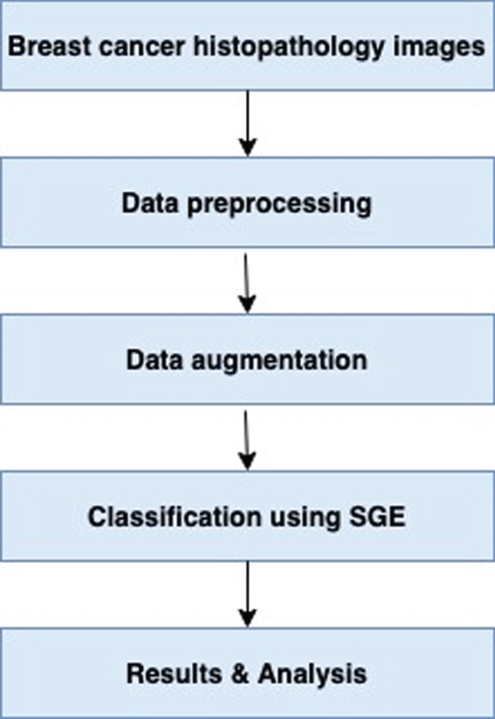
Flow diagram of the proposed methodology.

5.1 Dataset description

A histopathology breast cancer image dataset with IDC have been used for classification. The data is comprised of digitized breast cancer histopathological images with IDC. It has been the most prevalent subtype of all breast cancers specimens [58, 59]. It has 162 whole mount side images of IDC breast cancer. There is a total of 277,524 patches of images with 50x50 size out of which 198,738 are IDC- and 78,786 are IDC+[60]. The class distribution of the dataset has been depicted in Fig. 3 where IDC+represents the positive invasive ductal carcinoma while IDC- represents negative invasive ductal carcinoma. Figure 4 shows some samples of IDC- and IDC+patches taken from mount slides.

Fig. 3

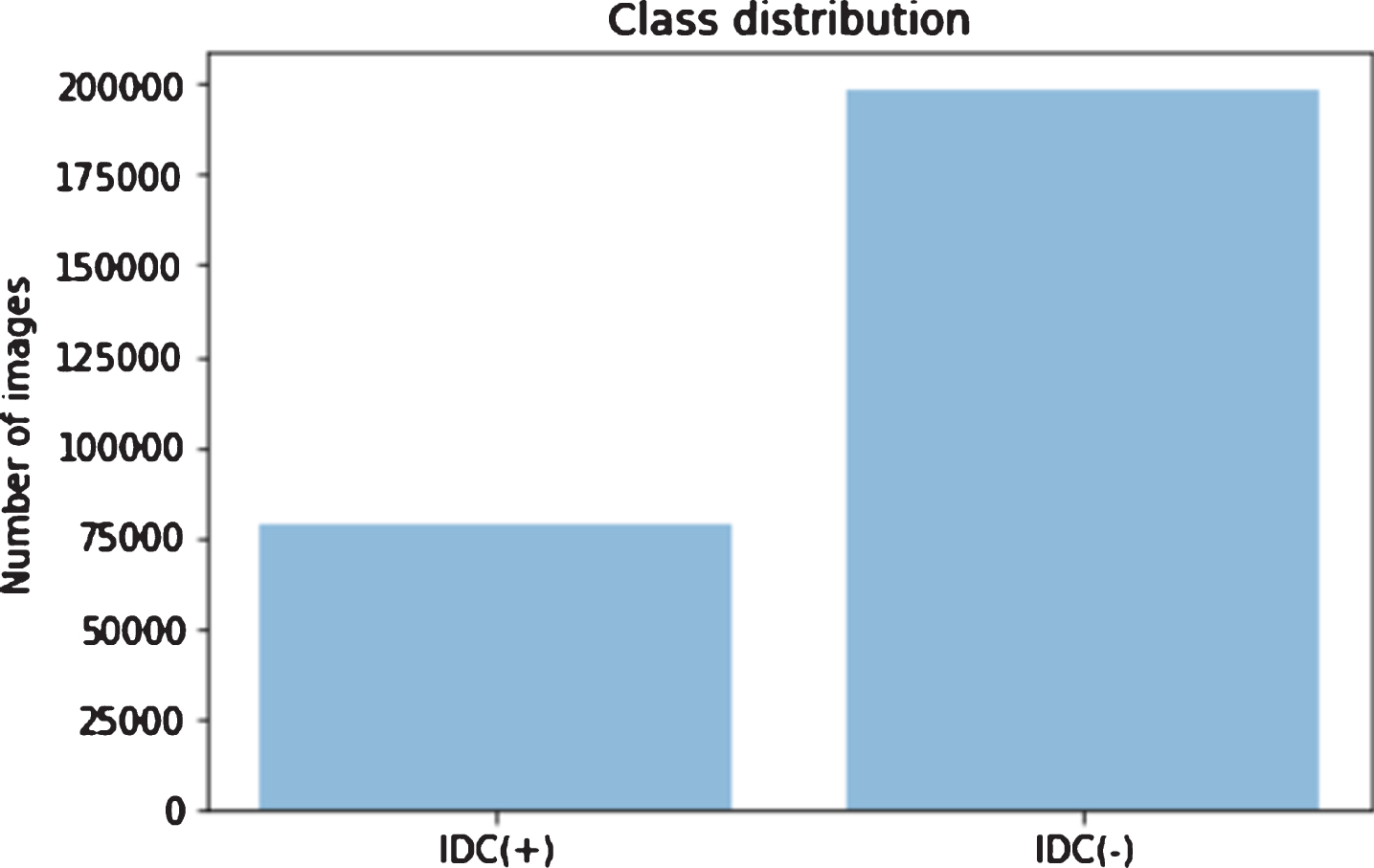
Class distribution of IDC (+) and IDC (-).

Fig. 4

A set of 9 samples from classes IDC+ and IDC- [60].

5.2 Data pre-processing

Data pre-processing is an important step in ML and DL. The data pre-processing step makes a model give better results. A csv file has been created for the dataset which uses the class labels that correspond to the index labels This was done using the csv writer package. Later on, the images were resized to 50×50 and interpolated using inter cubic interpolation [61]. The to_categorical() function is used for One-hot encoding the class labels as follows:

[1. 0.] = 0 for negative IDC;

[0. 1.] = 1 for positive IDC.

5.3 Data augmentation

The Model needs an introduction to variance to achieve a better scale as compared to aggregating the data in terms of increasing the size of the dataset. This can be achieved by using data Augmentation. Various data augmentation research has been studied for elucidating its use in nuances of the deep learning model proposed [62]. The model can be made using a different degree of variance for different images. The images had been subjected to different operations such as variances in size, variances in rotation with a range of 40 degrees, and variance in shear with a range of 0.4. These images also had a possibility for them to be flipped either vertically, or horizontally.

5.4 Model architecture

In this paper, the histopathology images are classified into IDC+ and IDC-. Many base models (six deep learning models i.e. CNN, DA, VGG16, VGG19, Xception (ReLu), Xception (Elu)) are used as level-0 model and one meta learner (Logistic Regression in this research) as level-1 model. The main motive of stack generalization is it learns from the predictions of level-0 models. The image size of 100x100 uniformity with batch size of 32 and kernel size of 3×3 has been taken for data augmentation model and basic CNN model.

The 1st model architecture for SGE which doesn’t utilize data augmentation. In the 1st model of the SGE convolutional layer (i.e. Conv2d_1) is the first layer and it has been taken as an input with a kernel size of (3,3), whereas ReLu (i.e. Rectified Linear Unit) activation function is introduced as a non-linearity. The equation for the Rectified Linear Unit has been given below in Equation (1). $\begin{matrix} Relu = 0 for x < 0 \\ = x for x ⩾ 0 \end{matrix}$ (1)

This layer gives 32 feature maps of sizes 50×50 in all. These feature maps are flattened (flatten_1) and then fed through a fully connected layer (dense_1) which has a feature space of 80000 features to 2 class outputs. It uses a softmax function for its final fully connected layer which gives class labels’ probabilities. This function has been shown in Equation (2). $σ {(z)}_{i} = \frac{e^{z_{i}}}{\sum_{j = 1}^{K} e^{z_{j}}}$ (2)

The model architecture of the proposed methodology is depicted in Fig. 5.

Fig. 5

The model architecture of the proposed methodology.

where i = 1, 2 ... , K and $z = (z_{1}, z_{2} \dots, z_{K}) \in ℝ^{k}$ .

The architecture of 2nd model for SGE uses normal CNN model that utilize data augmentation. This model also has its first convolutional layer (i.e. Conv2d_2) as an input with (3,3) kernel size with 32 filters and a stride of 2, along with ELu (i.e. Exponential Linear Unit) as an activation function. The equation for the ELu has been given below in Equation (3). $R (z) = {\begin{matrix} z Z < 0 \\ α (e^{z} - 1) Z ⩽ 0 \end{matrix}}$ (3) whereas α has value 1 as per Keras documentation. Matplotlib and Keras have been used for generating the figures [63, 64]. This model uses the augmentations that have been given below:

Shear range of 0.4;

Rotation range of 40°;

Width shift range of 0.4;

Height shift range of 0.4;

Zoom range of 0.4;

Horizontal and vertical shift; and

Rescaling to 255.

The first layer converts 100×100 image to 50×50 feature maps. This is then passed through the 0.15 dropout and then the max pooling layer (max pooling2d 1) reduces the size to 25×25. The second convolutional layer (conv2d 3) uses the same configuration as the 1st convolutional layer to display 6- character maps of 1313. Besides, a dropout of 0.25 was used after this layer (in dropout 2). A further 2 convolutional-dropout frames (conv2d 4, dropout 3, conv2d 5, dropout 4, respectively) with 0.35 and 0.45 dropouts with the same configuration as before were used to obtain 512 4×4-pixel maps each. These are then flattened (in flatten 2) to obtain 8192 values which are transferred through a fully connected layer of 120 neurons (in dense 2). The last dropout (dropout_5) of 0.35 has been introduced in this model which has then been passed through a fully connected layer (dense_3) to get the output as per one hot encoding defined earlier using softmax function (Equation (2)).

The architecture of 3rd model for SGE where VGG16 has transferred its weights from ImageNet dataset. Here, the VGG16 model has been pre-trained on ImageNet dataset for the input of 100×100. The weights obtained from VGG16 (vgg16_input) for this dataset (512 feature maps of 3×3) have been flattened (flatten_5) to get 4608 features which are then passed through a fully connected layer (dense_39) with 32 neurons through a dropout of 0.15 (in dropout_34). There are then 3 dense-dropout blocks (dense_40, dropout_35, dense_41, dropout_36, dense_42, dropout_37 in order) having 64, 128, 256 neurons and dropouts of 0.25, 0.35, 0.45, respectively. This model only utilizes ReLu (Equation (1) as its activation function in the block mentioned earlier. Finally, the output from 256 neurons has been passed through the final fully connected layer by a softmax activation function to get 2 outputs (Equation (2)).

The 4th model uses VGG19 model has been pre-trained on the ImageNet dataset for the input of 100×100. The weights obtained from VGG19 (vgg19_input) for this dataset (512 feature maps of 3×3) have been flattened (flatten_4) to get 4608 features which are then passed through a fully connected layer (dense_34) with 32 neurons through a dropout of 0.15 (in dropout_30). There are then 3 dense-dropout blocks (dense_35, dropout_31, dense_36, dropout_32, dense_37, dropout_33 in order) having 64, 128, 256 neurons and dropouts of 0.25, 0.35, 0.45, respectively. This model uses ReLu as an activation function in the block mentioned earlier. Finally, the output from 256 neurons has been passed through the final fully connected layer by a softmax activation function to get 2 outputs (Equation (2)).

The 5th model uses the pre-trained Xception model for input of 100×100. The weights obtained from Xception (xception_input) for this dataset (2048 feature maps of 3×3) have been flattened (flatten_6) to get 18432 features which are then passed through a fully connected layer (dense_44) with 32 neurons through a dropout of 0.15 (in dropout_38). There are then 3 dense-dropout blocks (dense_45, dropout_39, dense_46, dropout_40, dense_47, dropout_41 in order) having 64, 128, 256 neurons and dropouts of 0.25, 0.35, 0.45, respectively. This model uses ReLu as its activation function in the block mentioned earlier. Finally, the output from 256 neurons has been passed through the final fully connected layer (i.e. dense_48) by a softmax activation function to get 2 outputs (Equation (2)).

The 6th model has been pre-trained on the dataset of ImageNet for the input of 100×100. The weights obtained from Xception (Xception_input) for this dataset (2048 feature maps of 3×3) have been flattened (flatten_6) to get 18432 features which are then passed through a fully connected layer (dense_49) with 32 neurons through a dropout of 0.15 (in dropout_42). There are then 3 dense-dropout blocks (dense_50, dropout_43, dense_51, dropout_44, dense_52, dropout_45 in order) having 64, 128, 256 neurons and dropouts of 0.25, 0.35, 0.45, respectively. This model only utilizes an exponential linear unit (Equation (3)) as its activation function in the block mentioned earlier. The output of 256 neurons has been finally passed through the final fully connected layer by the softmax activation function to get 2 outputs (Equation (2)).

The graphs for all 5 of the activation functions mentioned from Equation (1 –3) are shown in Fig. 6(a-c), respectively.

The dataset from the 1st to 6th Model has been stacked for the SGE model. The stacked dataset is processed through Logistic Regression. The dstack() function is used for stacking together the output probabilities of 1st to 6th model.

Fig. 6

(a) A representation of Leaky Rectified Linear unit activation function; (b) A representation of softmax function. (c) A representation of the Exponential Linear Unit activation function.

SGE is inspired by the stacking models [65] which utilizes similar output predictions. The stacking models using Logistic regression layer as Level – 1 learner or meta – learner model whereas 1st to 6th models are sub-models or level 0 learner, have led to SGE. The predictions from new model and multiple existing models have been combines in SGE. Scikit-learn classifier as meta-learner and neural network as sub-model is used in this method for the stacked model.

Here

member is a list of all the models in the models’ directory;

inputX is test data set without any label;

b_test1, b_test2, b_test3, b_test4 are the bottleneck values for pretrained models

model is the final stacking generalized ensemble

The steps for the whole SGE algorithm have been described in the algorithm 1:

Algorithm 1: Stacked Generalised Ensemble

procedure STACKED_DATASET(models, X_test, bottlenecks)

stacked = None

For model in models

1 if model != pretrainedthen

2 Y = model.predict (X_test, Y_test)

3 else

4 Y = model.predict (bottleneck, X_test, Y_test)

6 ifstacked = None then

7 stacked = Y

8 else

9 stacked = dstack((stacked, Y))

10 continue

procedure FIT_STACKED_MODEL (models, X_test, Y_test,

bottlenecks)

stacked = stacked_dataset(models, X_test, bottlenecks)

model1 = LogisticRegression()

model1.fit(stacked)

return model1

6 Results and analysis

The detailed architecture of the proposed methodology has been discussed in section 3. The model performance has been evaluated on the basis of accuracy, precision, recall, F1-score for various classification algorithms.The classification model built using Keras and binary classification of images has been done into IDC+ & IDC-. Total 70,000 histopathology breast cancer images was trained and validated and tested on 30,000 images. The model had been run on 100 epochs. Each iteration uses binary cross entropy and Adam optimizer for loss calculation. Figures 7(a-f) & 8(a-f) depicts the sample classification images for class 0 and class1 whereas class 0 shows the IDC- and class 1 depicts IDC+.

Fig. 7(a-e)

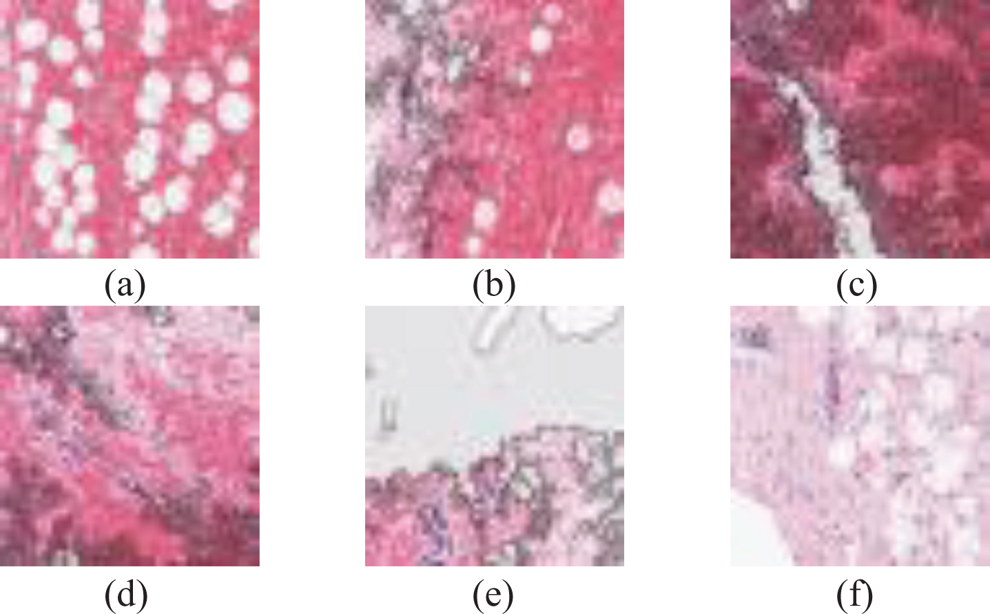
Sample of classified images with Class 0.

This section explains about the comparison and analysis of proposed Stacked Generalized Ensemble approach with various ML, DL and state-of-art methods.

6.1 Analysis using deep learning models

A detailed comparison of deep learning models like CNN, VGG16, VGG19, Xception (ReLu), Xception (Elu), Data Augmentations has been depicted in Table 3. CNN has achieved a minimum accuracy of 72.01% and SGE has achieved maximum accuracy of 87.80% whereas precision, recall, F1 score achieved for CNN is 0.52, 0.72, 0.60 respectively and.88 each for SGE.

Table 3
Performance comparison of deep learning models

Models Accuracy Precision Recall F1 score

CNN 0.72 0.52 0.72 0.60

VGG19 0.85 0.85 0.86 0.85

VGG16 0.85 0.86 0.86 0.86

Xception (ReLu) 0.84 0.85 0.85 0.85

Xception (ELu) 0.85 0.86 0.86 0.86

DA 0.86 0.86 0.87 0.87

SGE (LR) 0.87 0.88 0.88 0.88

Models	Accuracy	Precision	Recall	F1 score
CNN	0.72	0.52	0.72	0.60
VGG19	0.85	0.85	0.86	0.85
VGG16	0.85	0.86	0.86	0.86
Xception (ReLu)	0.84	0.85	0.85	0.85
Xception (ELu)	0.85	0.86	0.86	0.86
DA	0.86	0.86	0.87	0.87
SGE (LR)	0.87	0.88	0.88	0.88

The performance graph of validation loss & accuracy is depicted in Fig. 9. The performance graph of various deep learning models is shown in Fig. 10. The models have been run on 100 epochs with batch size 32.CNN resulted in training accuracy of.71 and training loss achieved is 4.61 while validation and testing accuracy had been maximized to 72% and 72.01% respectively. The validation loss for CNN has been recorded as 4.47 which shows CNN does not overfit the data. Figure 11(a-e) depicts the detailed model accuracy for the VGG16, VGG19, Xception (Relu), Xception (elu), CNN respectively.

Fig. 8(a-e)

Sample of classified images with Class 1.

Fig. 9

Performance Graph of validation loss and accuracy.

Fig. 10

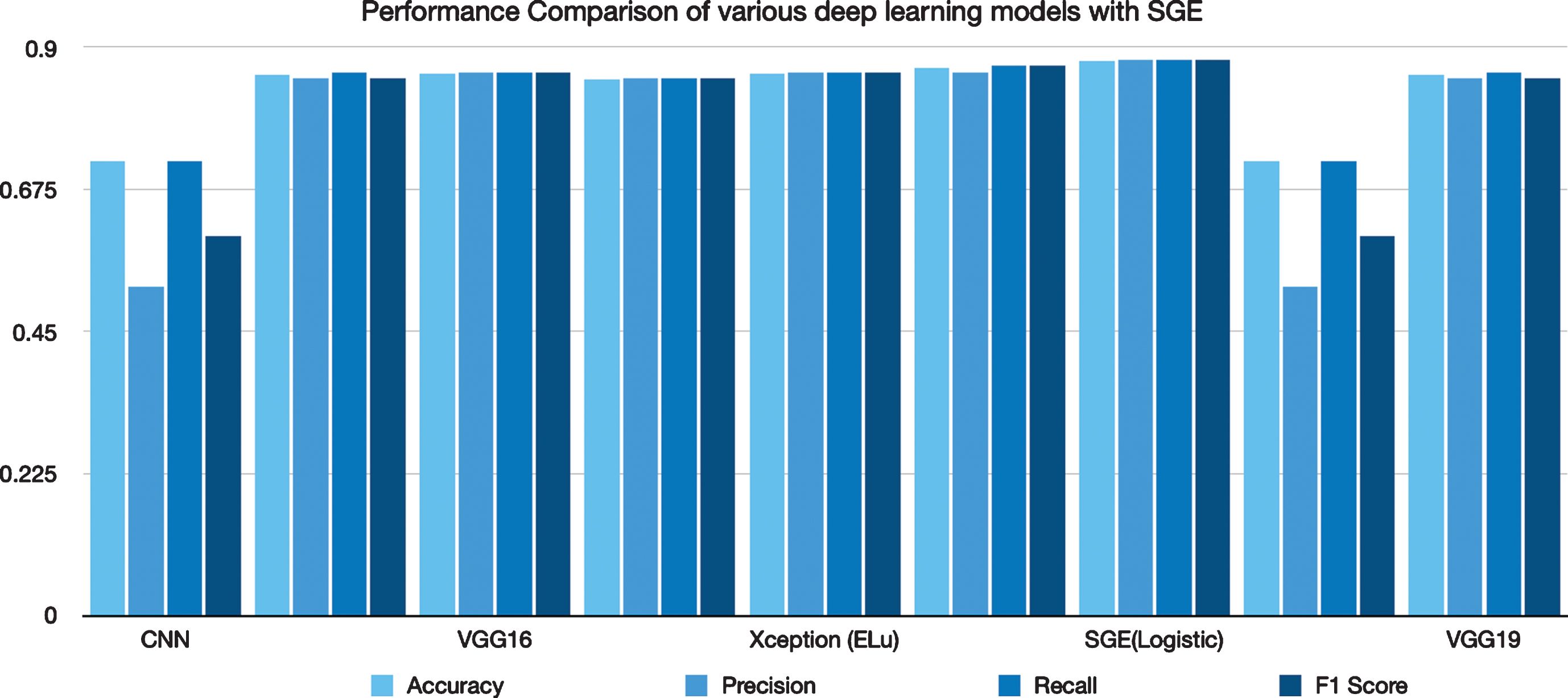
Performance Graph of deep learning models.

Fig. 11

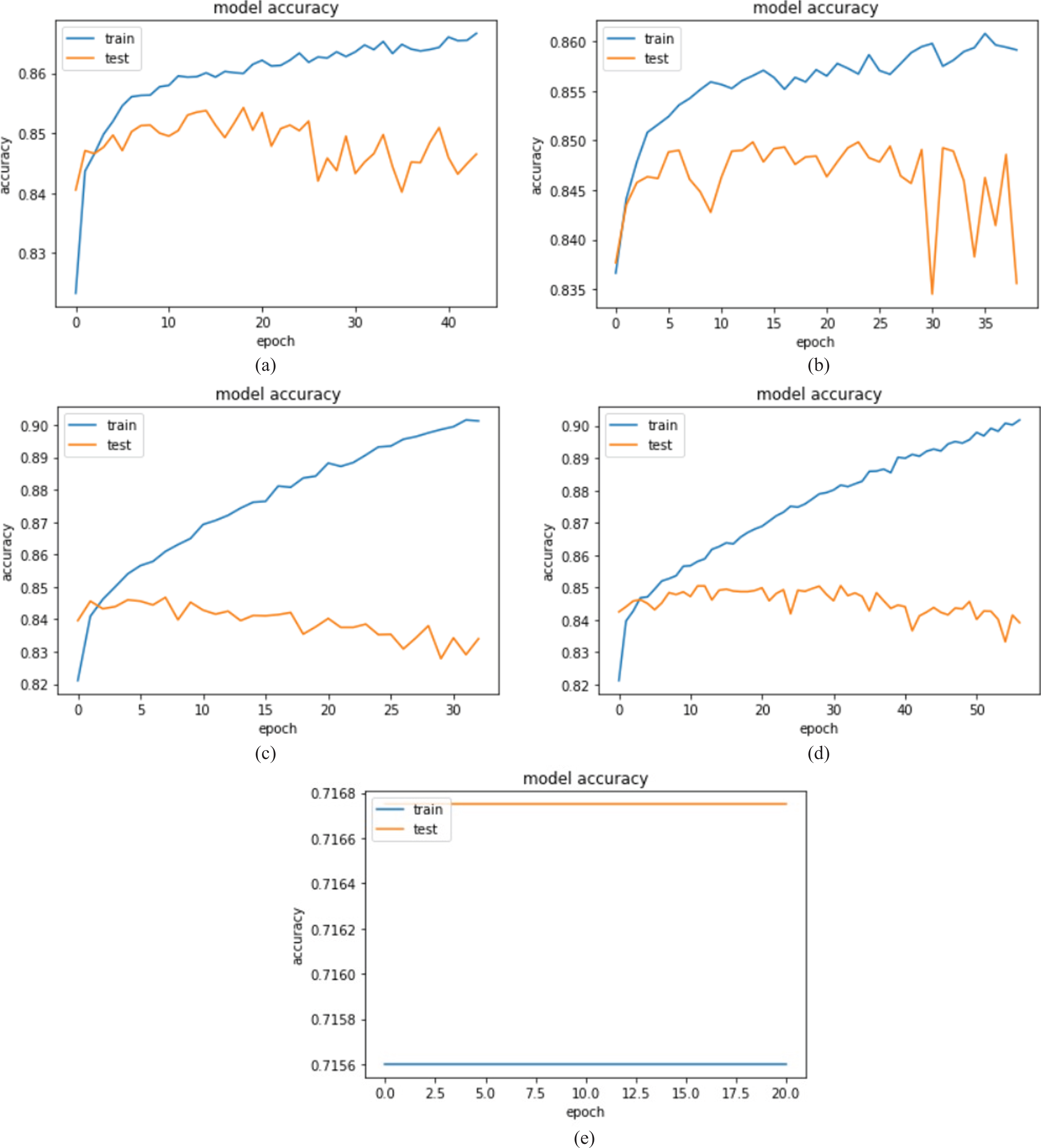
(a-e) Training accuracy of models – VGG16, VGG19, Xception (Relu), Xception (Elu), CNN.

Figure 12(a-e) depicts the detailed the model loss for the VGG16, VGG19, Xception (Relu), Xception (elu), CNN respectively.

Fig. 12

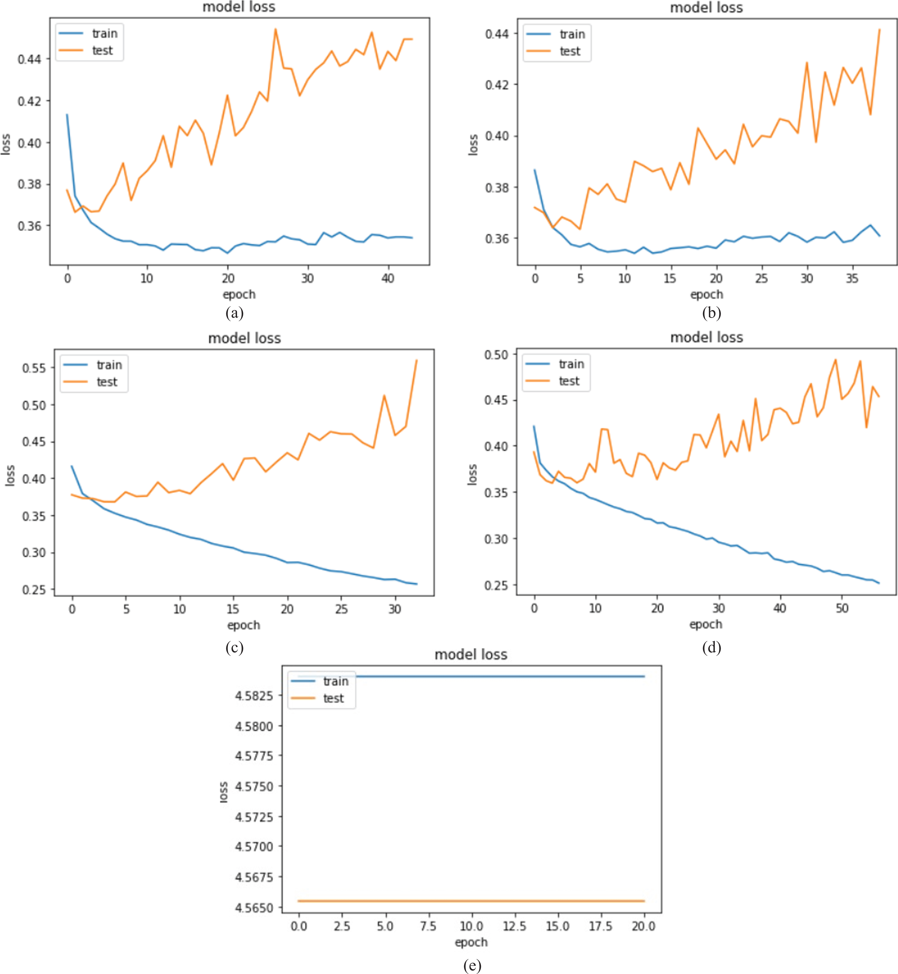
(a-e) Training loss of models – VGG16, VGG19, Xception (Relu), Xception (Elu), CNN.

Figure 13(a-f) illustrates the confusion matrix for the classification into IDC+ and IDC- by the number of models trained. Training of the model has been done on 70000 images, 12000 images have been used for validating trained models, and for testing 18000 images were used. CNN predicted 12817 images as IDC-, whereas 5183 as IDC+. Figure 14 illustrates the accuracy comparison of machine learning algorithms with the proposed algorithm SGE.

Fig. 13

(a-f) Confusion matrix for the two classes IDC+ & IDC–for CNN, VGG16, VGG19, Xception (ReLu), Xception (Elu), Data Augmentation.

Fig. 14

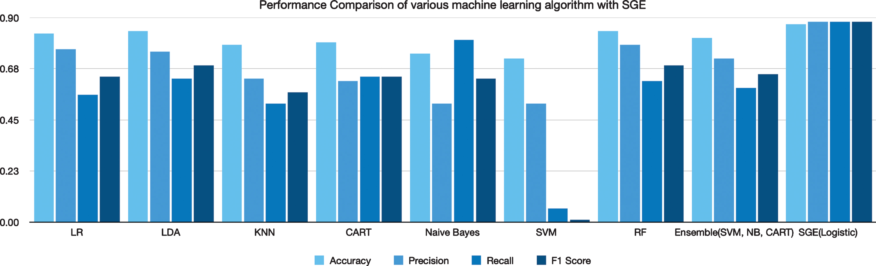
Accuracy comparison of machine learning algorithm with SGE.

6.2 Analysis using machine learning

In this subsection comparative analysis of various machine algorithm has been done.ML algorithms features are extracted using histograms, haralick feature extraction techniques. The classification algorithms are trained on these features. Furthermore, the performance of the Stacked Generalized Ensemble algorithm is compared with various ML algorithms like LR, LDA, KNN, CART, Naïve Bayes, SVM, Randaom Forest, and ensemble (SVM, Naïve Bayes, CART) [66 –69]. The proposed SGE performance has also been compared with an ensemble of three machine learning algorithms (SVM, NB, CART). The accuracy achieved by machine learning ensemble approach was 81% whereas SGE achieved maximum accuracy of 87.80%. Table 4 shows the detailed performance comparison of various machine learning algorithms. Figure 11 depicts the accuracy graph of the SGE algorithm with various machine learning algorithms and an ensemble of SVM, NB, CART. It has been illustrated well through the experiments and results that the proposed methodology performed more efficiently than the other existing methodologies.

Table 4
Performance comparison of ML algorithms with ensemble algorithm and proposed SGE

Models Accuracy Precision Recall F1 score

LR 0.83 0.76 0.56 0.64

LDA 0.84 0.75 0.63 0.69

KNN 0.78 0.63 0.52 0.57

CART 0.79 0.62 0.64 0.64

Naïve Bayes .74 .52 .80 .63

SVM 0.72 0.52 0.06 0.01

RF .84 .72 .59 .65

Ensemble (SVM, NB, CART) .81 .72 .59 .65

SGE (Logistic) 0.8780 0.88 0.88 0.88

Models	Accuracy	Precision	Recall	F1 score
LR	0.83	0.76	0.56	0.64
LDA	0.84	0.75	0.63	0.69
KNN	0.78	0.63	0.52	0.57
CART	0.79	0.62	0.64	0.64
Naïve Bayes	.74	.52	.80	.63
SVM	0.72	0.52	0.06	0.01
RF	.84	.72	.59	.65
Ensemble (SVM, NB, CART)	.81	.72	.59	.65
SGE (Logistic)	0.8780	0.88	0.88	0.88

6.3 Analysis using state-of-art methods

In this subsection the proposed methodology has been compared with the state-of-art methods. The detailed comparative analysis has been shown in Table 5. The proposed methodology using stacked Generalized Ensemble approach which utilizes six transfer learner model as level 0 learner and Logistic Regression as level 1 model. The proposed SGE outperformed the state-of-art methods.

Table 5
Proposed methodology accuracy comparison on IDC dataset

Source Authors Accuracy (%)

[70] Cruz-Roa et al. 84.23

[71] H. Alghodhaiifi et al. 86.1

[72] A Biswas et al. 86

[73] Mohapatra et al. 81

SGE (LR) – 87.8

Source	Authors	Accuracy (%)
[70]	Cruz-Roa et al.	84.23
[71]	H. Alghodhaiifi et al.	86.1
[72]	A Biswas et al.	86
[73]	Mohapatra et al.	81
SGE (LR)	–	87.8

The proposed methodology has been run on another breast cancer dataset. It has H&E (Hematoxylin-Eosin) stained images. The dataset used for experimentation is UCSB bio segmentation benchmark dataset. The proposed methodology achieved 97.5% accuracy on this dataset. The results for the same is depicted in Table 6:

Table 6

A comparative analysis of proposed methodology using H&E dataset [74]

Accuracy (%)	Precision (%)	Recall (%)	F1-Score (%)
97.5	98	98	98

7 Conclusion

It has been observed from the above-mentioned data that the results are inevitable that the proposed Stacked Generalized methodology achieves better results as compared to other existing techniques. It is an hour need to predict and diagnose cancer timely Therefore, if prediction accuracy can be increased by using computer aided techniques, it will be a great help to breast cancer treatment. SGE is inspired by the stacking models which utilize similar output predictions where the Logistic Regression layer is used as a meta-learner model or level 1 learner (or model) while 1st to 6th models are used as sub-models or level 0 learners. It is an ensemble method that combines the predictions from multiple existing models and a new model is learned. The breast cancer images are classified into cancerous and non-cancerous images. Accuracy has been taken as the main evaluation criteria for various classification algorithms. Furthermore, the performance of the Stacked Generalized Ensemble algorithm is compared with various ML algorithms like LR, LDA, KNN, CART, Naïve Bayes, SVM, and an ensemble of SVM, Naïve Bayes, CART. The proposed SGE performance has also been compared with an ensemble of three machine learning algorithms (SVM, NB, CART). The accuracy achieved by machine learning algorithms was 81% whereas SGE achieved maximum accuracy of 87.80%. It has been illustrated well through the experiments and results that the proposed methodology performed more efficiently than the other existing methodologies. Thus, the proposed approach is appropriate for breast cancer image classification in real-time applications.

References

Ferlay

, Héry

, Autier

and Sankaranarayanan

, Global burden of breast cancer, in Breast Cancer Epidemiology, Springer New York, 2010, pp. 1–19.

Zaidi

and Dib

H.A.

, Abstract: The worldwide female breast cancer incidence and survival, 2018 (2019), 4191–4191.

Youlden

D.R.

, Cramb

S.M.

, Yip

C.H.

and Baade

P.D.

, Incidence and mortality of female breast cancer in the Asia-Pacific region, Cancer Biol Med 11(2) (2014), 101–115.

World Health Organization. Accessed: Mar. 10, 2018. Available: http://www.who.int/en/breast cancer.

Stewart

and Wild

C.P.

, and (Eds), IARC Publications Website – World Cancer Report 2014. 2014.

Kumar

and Batra

, Epidemiology of breast cancer in indian women: Population and hospital based study, EAI Endorsed Trans Pervasive Heal Technol 4(16) (2018).

Joy

, Penhoet

and Petitti

, Saving women’s lives: strategies for improving breast cancer detection and diagnosis, 2005.

Cheng

H.D.

, Shan

, Ju

, Guo

and Zhang

, Automated breast cancer detection and classification using ultrasound images: A survey, Pattern Recognit 43 (2010), 299–317.

, Wang

, Liu

, Latecki

L.J.

, Wang

and Huang

, Weakly supervised mitosis detection in breast histopathology images using concentric loss, Med Image Anal 53 (2019), 165–178.

10.

Wahab

, Khan

and Lee

Y.S.

, Transfer learning based deep CNN for segmentation and detection of mitoses in breast cancer histopathological images, Microscopy 68(3) (2019), 216–233.

11.

Cowherd

S.M.

, Tumor staging and grading: A primer, Methods Mol Biol 823 (2012), 1–18.

12.

, Long

L.R.

, Antani

and Thoma

G.R.

, Histology image analysis for carcinoma detection and grading, Comput Methods Programs Biomed 107(3) (2012), 538–556.

13.

Deeb

S.J.

, Tyanova

, Hummel

, Schmidt-Supprian

, Cox

and Mann

, Machine Learning-based Classification of Diffuse Large B-cell Lymphoma Patients by Their Protein Expression Profiles S, Mol Cell Proteomics 14 (2015), 2947–2960.

14.

Yassin

, Omran

, . . . E.E. H.-C. methods and, and undefined 2018, Machine learning techniques for breast cancer computer aided diagnosis using different image modalities: A systematic review, Elsevier.

15.

Al-antari

M.A.

, Al-masni

M.A.

, Choi

M.T.

, Han

S.M.

and Kim

T.S.

, A fully integrated computer-aided diagnosis system for digital X-ray mammograms via deep learning detection, segmentation, and classification, Int J Med Inform 117 (2018), 44–54.

16.

Yang

Z.R.

, Biological applications of support vector machines, Briefings in bioinformatics 5(4) (2004), 328–338.

17.

Datta

, Feature selection and machine learning with mass spectrometry data, Methods Mol Biol 1007 (2013), 237–262.

18.

Wang

, et al., Gene selection from microarray data for cancer classification-a machine learning approach, Comput Biol Chem 29 (2005), 37–46.

19.

Cai

, Xu

, Zhang

, Ngai

S.M.

and Shao

, Classification of lung cancer using ensemble-based feature selection and machine learning methods, Mol Biosyst 11(3) (2015), 791–800.

20.

Bonilla Huerta

, Duval

and Hao

J.K.

, A hybrid LDA and genetic algorithm for gene selection and classification of microarray data, Neurocomputing 73(13–15) (2010), 2375–2383.

21.

Kittler

, Hatef

, Duin

R.P.W.

and Matas

, On Combining Classifiers, 1998.

22.

Janghel

R.R.

, Shukla

, Sharma

and Gnaneswar

A.V.

, Evolutionary ensemble model for breast cancer classification, in, Lecture Notes in Computer Science (including subseries Lecture Notes in Artificial Intelligence and Lecture Notes in Bioinformatics) 8795 (2014), 8–16.

23.

Kassani

S.H.

, Kassani

P.H.

, Wesolowski

M.J.

and Schneider

K.A.

, Classification of Histopathological Biopsy Images Using Ensemble of Deep Learning Networks, arxiv.org.

24.

Shoaib

, Sehgal

, Gondal

and Dooley

, Stacked Regression Ensemble for Cancer Class Prediction, ieeexplore-ieee-org.web.bisu.edu.cn, 2005.

25.

Khan

M.J.

, Khurshid

and Charan

, Breast Cancer Detection in Mammograms using Convolutional Neural Network, ieeexplore-ieee-org.web.bisu.edu.cn.

26.

Khan

, Wahab

and Lee

Y.S.

, Two-phase deep convolutional neural network for reducing class skewness in histopathological images based breast cancer detection, Artic Comput Biol Med, 2017.

27.

Desai

, Biomedical Data Classification with Improvised Deep Learning Architectures, Comput Sci Diss, Aug. 2020.

28.

Allah

, Abd El Zaher

, Eldeib

A.M.

and Abdel-Zaher

A.M.

, Breast cancer classification using deep belief networks, Expert Syst Appl 46 (2016), 139–144.

29.

LeCun

, Bengio

, G.H.-nature, and undefined 2015, Deep learning, nature.com, 2015.

30.

Krizhevsky

, Sutskever

and Hinton

G.E.

, ImageNet classification with deep convolutional neural networks, Commun ACM 60(6) (2017), 84–90.

31.

Simonyan

and Zisserman

, VERY DEEP CONVOLUTIONAL NETWORKS FOR LARGE-SCALE IMAGE RECOGNITION, 2015.

32.

Kowal

, Filipczuk

, Obuchowicz

, Korbicz

and Monczak

, Computer-aided diagnosis of breast cancer based on fine needle biopsy microscopic images, Comput Biol Med 43(10) (2013), 1563–1572.

33.

Zhang

, Zhang

, Coenen

, Xiao

and Lu

, One-class kernel subspace ensemble for medical image classification, EURASIP J Adv Signal Process 2014(1) (2014).

34.

Wang

, Hu

, Li

, Liu

and Zhu

, Automatic cell nuclei segmentation and classification of breast cancer histopathology images, Signal Processing 122 (2016), 1–13.

35.

Spanhol

F.A.

, Oliveira

L.S.

, Petitjean

and Heutte

, A Dataset for Breast Cancer Histopathological Image Classification, IEEE Trans Biomed Eng 63(7) (2016), 1455–1462.

36.

Al-Hadidi

M.R.

, Alarabeyyat

and Alhanahnah

, Breast Cancer Detection Using K-Nearest Neighbor Machine Learning Algorithm, in Proceedings – 2016 9th International Conference on Developments in eSystems Engineering, DeSE 2016, 2017, pp. 35–39.

37.

Chen

, Dou

, Wang

, Qin

and Heng

P.A.

, Mitosis detection in breast cancer histology images via deep cascaded networks, in 30th AAAI Conference on Artificial Intelligence, AAAI 2016, 2016, pp. 1160–1166.

38.

Filipczuk

, Fevens

, Krzyzak

and Monczak

, Computer-aided breast cancer diagnosis based on the analysis of cytological images of fine needle biopsies, IEEE Trans Med Imaging 32(12) (2013), 2169–2178.

39.

Doyle

, et al., Automated gland and nuclei segmentation for grading prostate and breast cancer histopathology, ieeexplore-ieee-org.web.bisu.edu.cn, 2008.

40.

Bayramoglu

, Kannala

and Heikkila

, Deep learning for magnification independent breast cancer histopathology image classification, in Proceedings - International Conference on Pattern Recognition, 2016, pp. 2440–2445.

41.

Shelhamer

, Long

and Darrell

, Fully Convolutional Networks for Semantic Segmentation, IEEE Trans Pattern Anal Mach Intell 39(4) (2017), 640–651.

42.

Szegedy

, et al., Going deeper with convolutions, in Proceedings of the IEEE Computer Society Conference on Computer Vision and Pattern Recognition, 2015, vol. 07- 12-June, pp. 1–9.

43.

Esteva

, et al., Dermatologist-level classification of skin cancer with deep neural networks, Nature 542(7639) (2017), 115–118.

44.

Szegedy

, Vanhoucke

, Ioffe

, Shlens

and Wojna

, Rethinking the InceptionArchitecture for ComputerVision, in Proceedings of the IEEE Computer Society Conference on Computer Vision and Pattern Recognition, 2016, vol. 2016-Decem, pp. 2818–2826.

45.

, Zhang

, Ren

and Sun

, Delving deep into rectifiers: Surpassing human-level performance on imagenet classification, in Proceedings of the IEEE International Conference on Computer Vision, 2015, vol. 2015 Inter, pp. 1026–1034.

46.

Al Nahid

, Mehrabi

M.A.

and Kong

, Histopathological breast cancer image classification by deep neural network techniques guided by local clustering, Biomed Res Int 2018 (2018).

47.

Araujo

, et al., Classification of breast cancer histology images using convolutional neural networks, PLoS One 12(6) (2017).

48.

Han

, Wei

, Zheng

, Yin

, Li

and Li

, Breast Cancer Multi-classification from Histopathological Images with Structured Deep Learning Model, Sci Rep 7(1) (2017).

49.

Belsare

A.D.

, Mushrif

M.M.

, Pangarkar

M.A.

and Meshram

, Classification of breast cancer histopathology images using texture feature analysis, in IEEE Region 10 Annual International Conference, Proceedings/TENCON, 2016, vol. 2016-Janua.

50.

Ferreira

C.A.

, et al., Classification of Breast Cancer Histology Images Through Transfer Learning Using a Pre-trained Inception Resnet V2, Springer, vol. 10882 LNCS, pp. 763–770, 2018.

51.

Kwok

, Multiclass Classification of Breast Cancer in Whole-Slide Images, in Lecture Notes in Computer Science (including subseries Lecture Notes in Artificial Intelligence and Lecture Notes in Bioinformatics), 2018, vol. 10882 LNCS, pp. 931–940.

52.

Ting

and Witten

, Stacked Generalization: when does it work? 1997.

53.

Džeroski

and Ženko

, Is combining classifiers with stacking better than selecting the best one? Mach Learn 54(3) (2004), 255–273.

54.

Ting

K.M.

and Witten

I.H.

, Issues in Stacked Generalization, 1999.

55.

Yaşar

, M.C. M. I. and H. Informatics, and undefined 2016, A novel approach for reduction of breast tissue density effects on normal and abnormal masses classification, ingentaconnect.com.

56.

Rakhlin

, Shvets

, Iglovikov

and Kalinin

A.A.

, Deep Convolutional Neural Networks for Breast Cancer Histology Image Analysis, in Lecture Notes in Computer Science (including subseries Lecture Notes in Artificial Intelligence and Lecture Notes in Bioinformatics), 2018, vol. 10882 LNCS, pp. 737–744.

57.

Coccia

, Deep learning technology for improving cancer care in society: New directions in cancer imaging driven by artificial intelligence, Technol Soc 60 (2020), 101198.

58.

Janowczyk

and Madabhushi

, Deep learning for digital pathology image analysis: A comprehensive tutorial with selected use cases, J Pathol Inform 7(1) (2016).

59.

Narayanan

B.N.

, Krishnaraja

and Ali

, Convolutional Neural Network for Classification of Histopathology Images for Breast Cancer Detection, in Proceedings of the IEEE National Aerospace Electronics Conference, NAECON, 2019, vol. 2019-July, pp. 291–295.

60.

Breast Histopathology Images | Kaggle. [Online]. Available: https://www.kaggle.com/paultimothymooney/breast-histopathology-images. [Accessed: 03-Oct-2020].

61.

Sarfraz

, Visualization of positive and convex data by a rational cubic spline interpolation, Inf Sci (Ny) 146(1–4) (2002), 239–254.

62.

Dosovitskiy

, Springenberg

J.T.

and Brox

, Unsupervised feature learning by augmenting single images, in 2nd International Conference on Learning Representations, ICLR 2014 - Workshop Track Proceedings, 2014.

63.

, Yan

, Shan

, Dang

and Sun

, Deep Image: Scaling up Image Recognition, academia.edu, 2015.

64.

Hunter

J.D.

, Matplotlib: A 2D graphics environment, Comput Sci Eng 9(3) (2007), 90–95.

65.

Wolpert

D.H.

, Stacked generalization, Neural Networks 5(2) (1992), 241–259.

66.

Suykens

J.A.K.

and Vandewalle

, Least squares support vector machine classifiers, Neural Process Lett 9(3) (1999), 293–300.

67.

Rish

, IBM Technical Report RC22230: An empirical study of the naive Bayes classifier, 2001.

68.

Ben-Haim

and Com

Y.I.

, A Streaming Parallel Decision Tree Algorithm Elad Tom-Tov, 2010.

69.

A.L. and Wiener

, Classification and Regression by random Forest. R News 2, vol. 3, no. December 2002. pp. 18–22, 2003.

70.

Cruz-Roa

, et al., Automatic detection of invasive ductal carcinoma in whole slide images with convolutional neural networks, in, Medical Imaging 2014: Digital Pathology 9041 (2014), 904103.

71.

Zhu

, Song

, Wang

, Dong

, Guo

and Liu

, Breast cancer histopathology image classification through assembling multiple compact CNNs, BMC Med Inform Decis Mak 19(1) (2019).

72.

Biswas

, Al Nazi

and Abir

T.A.

, Invasive Ductal Carcinoma Detection by A Gated Recurrent Unit Network with Self Attention, in 2019 4th International Conference on Electrical Information and Communication Technology, EICT 2019, 2019.

73.

Mohapatra

, Panda

and Swain

, Enhancing histopathological breast cancer image classification using deep learning, Int J Innov Technol Explor Eng 8(7) (2019), 2024–2032.

74.

Bio-Segmentation | Center for Bio-Image Informatics | UC Santa Barbara. [Online]. Available: https://bioimage.ucsb.edu/research/bio-segmentation.

Classification of Invasive Ductal Carcinoma from histopathology breast cancer images using Stacked Generalized Ensemble

Abstract

Keywords

1 Introduction

2 Related work

3 Stack generalization framework

Table 1 Comparative analysis of various ML algorithms Models Accuracy Logistic Regression 83.15% Linear Discriminant Analysis 84.09% KNN 78.16% CART 79.53% RF 84% Naïve Bayes 74.23% SVM 72.31%

5.3 Data augmentation

5.4 Model architecture

Table 3 Performance comparison of deep learning models Models Accuracy Precision Recall F1 score CNN 0.72 0.52 0.72 0.60 VGG19 0.85 0.85 0.86 0.85 VGG16 0.85 0.86 0.86 0.86 Xception (ReLu) 0.84 0.85 0.85 0.85 Xception (ELu) 0.85 0.86 0.86 0.86 DA 0.86 0.86 0.87 0.87 SGE (LR) 0.87 0.88 0.88 0.88

Table 5 Proposed methodology accuracy comparison on IDC dataset Source Authors Accuracy (%) [70] Cruz-Roa et al. 84.23 [71] H. Alghodhaiifi et al. 86.1 [72] A Biswas et al. 86 [73] Mohapatra et al. 81 SGE (LR) – 87.8

References

Table 1
Comparative analysis of various ML algorithms

Models Accuracy

Logistic Regression 83.15%

Linear Discriminant Analysis 84.09%

KNN 78.16%

CART 79.53%

RF 84%

Naïve Bayes 74.23%

SVM 72.31%

Table 5
Proposed methodology accuracy comparison on IDC dataset

Source Authors Accuracy (%)

[70] Cruz-Roa et al. 84.23

[71] H. Alghodhaiifi et al. 86.1

[72] A Biswas et al. 86

[73] Mohapatra et al. 81

SGE (LR) – 87.8