
Abstract
In agricultural production, weed removal is an important part of crop cultivation, but inevitably, other plants compete with crops for nutrients. Only by identifying and removing weeds can the quality of the harvest be guaranteed. Therefore, the distinction between weeds and crops is particularly important. Recently, deep learning technology has also been applied to the field of botany, and achieved good results. Convolutional neural networks are widely used in deep learning because of their excellent classification effects. The purpose of this article is to find a new method of plant seedling classification. This method includes two stages: image segmentation and image classification. The first stage is to use the improved U-Net to segment the dataset, and the second stage is to use six classification networks to classify the seedlings of the segmented dataset. The dataset used for the experiment contained 12 different types of plants, namely, 3 crops and 9 weeds. The model was evaluated by the multi-class statistical analysis of accuracy, recall, precision, and F1-score. The results show that the two-stage classification method combining the improved U-Net segmentation network and the classification network was more conducive to the classification of plant seedlings, and the classification accuracy reaches 97.7%.
Introduction
In agricultural production, weed invasion is an unavoidable problem, and people use various methods to control weeds. So far, the main methods of removing weeds are physical, chemical and rational planting. Physical weeding means that people use machinery to artificially remove weeds, but the disadvantage of this method is that it requires the manual identification of weeds and crops. Chemical weeding is the use of pesticides and other chemicals to suppress weeds, but pesticides not only kill weeds, but also remain on the surface of crops, thus endangering people’s health. Rational planting reduces the growth of weeds by reducing the open space through close planting. Planting cover crops between crops eliminates the space to prevent weeds from growing, and prevents light from entering weed seeds to inhibit their growth. However, this kind of planting method requires conducting a certain amount of research on agronomy, which is more difficult for farmers. Therefore, how to reduce artificial identification in the process of physical weeding is a problem, and the development of deep learning allows for seeking a solution. How to identify and remove weeds at the seedling stage of weeds and crops is a research direction.
Therefore, the classification of plant seedlings has always been a focus. Most researchers use the existing classification network model to classify plant seedlings. With the continuous development of deep learning technology, many excellent classification network models have emerged. However, in the classification research of plant seedlings, the method of fine-tuning the existing classification network model is mostly used to improve the classification performance of plant seedlings.
In 2013, Zhao Zhang et al. proposed a plant leaf identification method based on PCA and SVM. After the segmentation and edge detection of a leaf image, 10 characteristic parameters of the leaf with rotation, scale, and translation invariance were extracted, principal component analysis was performed on these parameters, and the first three principal components were used as support vectors. The input of the machine establishes a pattern recognition model. The algorithm has an accuracy rate of 97.22% for the recognition of four plant leaves, namely, privet, papaya, five-cornered maple, and triangular maple [1]. At the same time, Jiao Ding et al. proposed a method based on weighted local linear embedding (WLLE) and support vector for the problem that the local linear embedding (LLE) algorithm is susceptible to noise and the nearest neighbor classifier cannot effectively identify plant leaves. In the support-vector machine (SVM) method of plant leaf identification, experimental data used 220 kinds of plants, a total of 16846 plant leaf images. Infant azulene leaves were selected as the positive samples, and an average accuracy rate of 98.16% was obtained [2].
In 2016, Mads Dyrmann et al. used a new CNN structure to classify species of plant seedlings. The author chose 2–10 days old plant seedlings, borrowing from the residual structure in resnet50, using the transfer learning method to obtain the initial parameters, and the average accuracy of the final classification was 86.2% [3].
In 2017, Thomas Mosgaard Giselsson et al. of the Signal Processing Group of Aarhus University and the University of Southern Denmark established a benchmark public image database of plant seedling classification algorithms, including 5539 images, divided into 12 species (3 crops and 9 kinds of weeds), image data were all captured at the early growth stage of seedlings. Their work provides a unified dataset for the classification of plant seedlings [4]. Therefore, in 2018, Trupti R. Chavan et al. established the AgroAVNET structure based on AlexNet (Krizhevsky et al., 2012) and VGGNET (Simonyan and Zisserman, 2014) to classify crops and weeds. This is a public dataset established by Thomas Mosgaard Giselsson et al. The average accuracy of the final classification of the AgroAVNET structure was 93.64% [5].
At the same time, the CNN developed by Heba A. Elnemr et al. is based on a hybrid model of AlexNet and VGG-Net. The normalization concept of the network was inspired by AlexNet, and the depth of the filter is selected on the basis of VGG-Net. Similarly, the author used a publicdataset created by Thomas Mosgaard Giselsson et al., with an average accuracy of classification of 94.38% [6].
In addition, Daniel Nkemelu et al. compared the effects of traditional algorithms and CNN on this dataset, and performed background removal. The traditional algorithms were KNN and SVM. After preprocessing the dataset for de-backgrounding, the final classification’s average accuracy rates were 56.84% and 61.47% respectively. Using CNN to train on the dataset without background removal and without background removal, average accuracy rates of 80.21% and 92.60% were obtained [7].
Moreover, Seo Jeong Kim et al. used an onion field dataset for weed classification research. The author classified crops and weeds into two categories, and did not subdivide the weeds. The crops were only onions, and the CNN network was its own. The final average accuracy rate was 99% [8]. Shubo Wang et al. identified corn, peanuts, wheat and three kinds of weeds. The dataset used plants that the authors had photographed. With the author’s own CNN network, the final average accuracy rate reached 95.6% [9].
After that, Belal A. M. Ashqar et al. used the VGG16 network to classify the public dataset of plant seedlings in 2019. The author performed feature extraction on the dataset, and on this basis, studied the impact on plant classification under the conditions of not changing the number of each type of dataset and using data enhancement to make the number of each type of dataset equal, obtaining 98.57 % accuracy [10]. Catherine R. Alimboyong et al. used AlexNet, VGG16, GoogLeNet, and ResNet networks to classify this public dataset. Each network used migration learning, and the final accuracy rate reached 90.5% [11].
Lastly, in 2020, Vo Hoang Trong et al. also used ResNet and VGG, and added network models such as NASNet, Inception–Resnet, and Mobilenet. They classified the public dataset of plant seedlings, and accuracy was 97.31% [12]. In order to classify plants and weeds, Nawmee Razia Rahman et al. used LeNet-5, VGG-16, DenseNet-121, and ResNet-50 to find the best-performing model, and obtained results of 96.21% [13]. In addition, Keshav Gupta et al. used ResNet50, VGG16, VGG19, Xception and MobileNetV2 to classify public datasets, and the best model was resnet50 with accuracy of 95.23% [14].
On the basis of the above-mentioned work, researchers aimed to improve or fine-tune a certain classification network in the classification of plant seedlings. The effect of using a classification network is not ideal. Therefore, this paper proposes a new method to improve seedling classification performance that combines the improved U-Net and other classification models, and was a two-stages: first, using the improved U-Net network to segment the target data, removing the background information, and then using the classification network to classify the seedlings.
The organizational structure of this article is as follows: Section 1 is the general overview of the method, including the U-Net and improved U-Net segmentation models, InceptionV3 and other classification models; Section outlines the experimental results; Section 3 compares the algorithm performance; Section 4 is the discussion; Section 5 is the conclusion.
Materials and methods
This section mainly details the classification methods of crops and weeds. This section is divided into four parts: image acquisition and preprocessing, image segmentation, image classification, and evaluation. The overall architecture is shown in Fig. 1. The image acquisition and preprocessing module unifies the format of the original dataset, unifying all pictures into 24-bit pictures, with a size of 512×512, which is the U-Net network input size. The image segmentation module performs three different operations on the dataset after the format is unified, that is, the improved U-Net network is used to segment the image data, and the original U-Net network is used to segment the image data without any processing. The image classification module uses three differently processed datasets to train the six networks of InceptionV3, Resnet50, NASnet, MobilenetV2, Densenet121, and Se-Resnet50. The model evaluation module uses accuracy, recall, precision and F1-score to evaluate 18 results.

The overall architecture of the deep learning method for plant seedlings.
The dataset for this experiment uses a public dataset that contains 5537 images of 12 kinds of plants, namely, 3 kinds of crops and 9 kinds of weeds, as shown in Fig. 2. According to the conclusions obtained by Sharada Prasanna Mohanty, we divided the dataset proportions into a 90% training set and a 10% test set [15], as shown in Table 1.
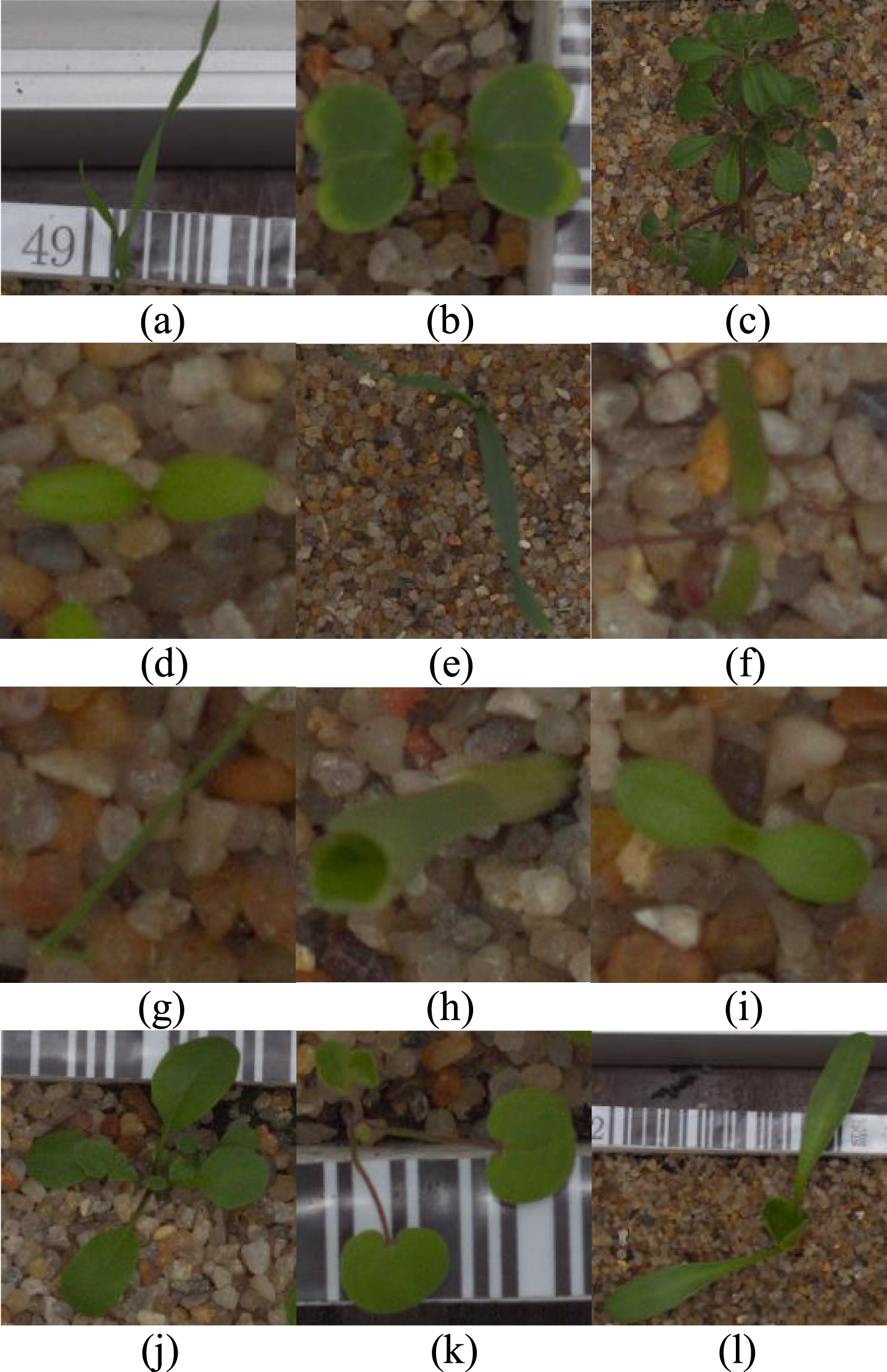
Sample images. (a) black grass. (b) charlock. (c) cleavers. (d) common chickweed. (e) common wheat. (f) fat hen. (g) loose silky bent. (h) maize. (i) scentless mayweed. (j) shepherd purse. (k) small flowered cranesbill. (l) sugar beet.
Dataset details
When preprocessing the image, since the resolution of the original image was different, we first unified the size of the image. Since the picture input size of the U-net network is 512×512 [16], in the preprocessing stage, we unified the picture resolution to 512×512. Next, we manually inspected the processed pictures, removed the damaged pictures, and converted the 32-bit pictures into 24-bit ones. The final number of obtained pictures was 5537.
Next, we performed three different processes on the dataset, and the picture after image segmentation is shown in Fig. 3. The first is not to perform any processing; the second is to use the original U-net to segment the dataset (with the BN layer added), and the network structure is shown in Fig. 4; the third is to use the improved U-net segmentation dataset, and the network structure is shown in Fig. 5. The purpose of data segmentation here is to remove image background interference and extract the seedling targets. Comparing Fig. 3, on the basis of the original U-net, whether it was down or up-sampling, at each scale, we increased the number of convolutional layers. For the first scale, we increased the number of convolutional layers to 3, and for the other scales, we increased the number of convolutional layers to 4, and added a BN layer after each convolutional layer.
We used the hyperparameters for the two U-nets, shown in Table 2.
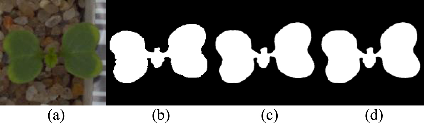
(a) Original image. (b)Ground truth. (c) Image after Original U-net segmentation. (d) Image after improved U-net segmentation.
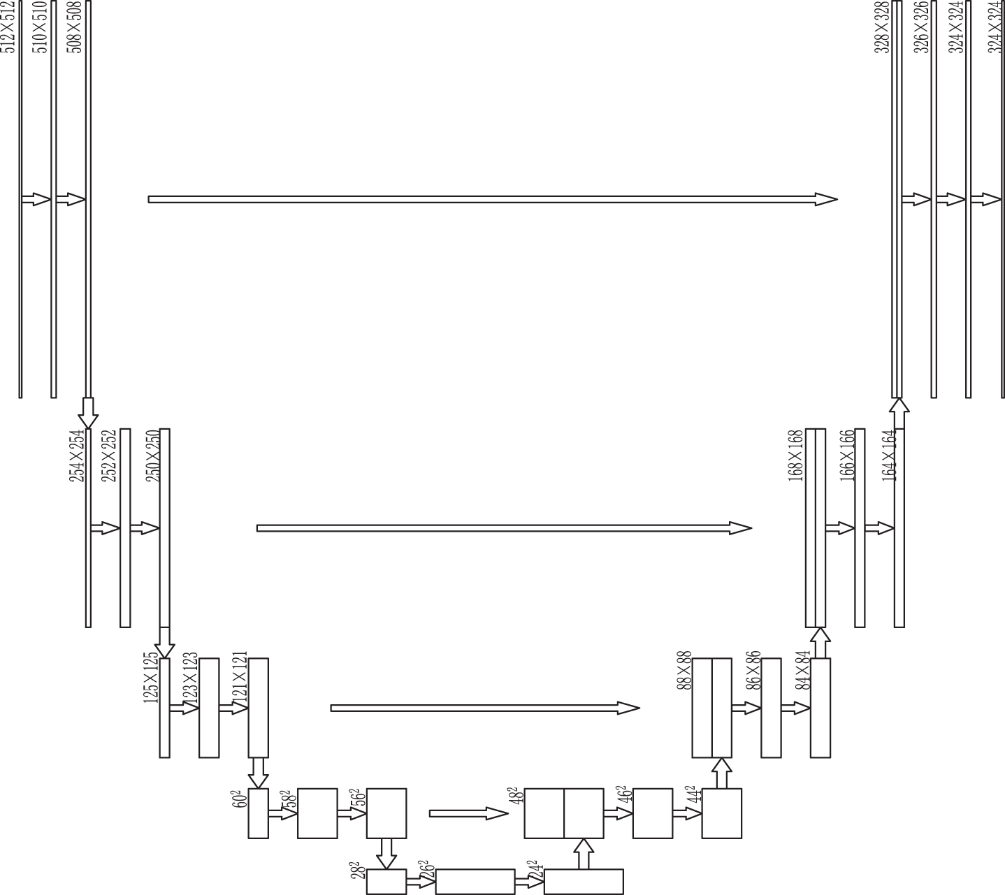
U-net architecture.
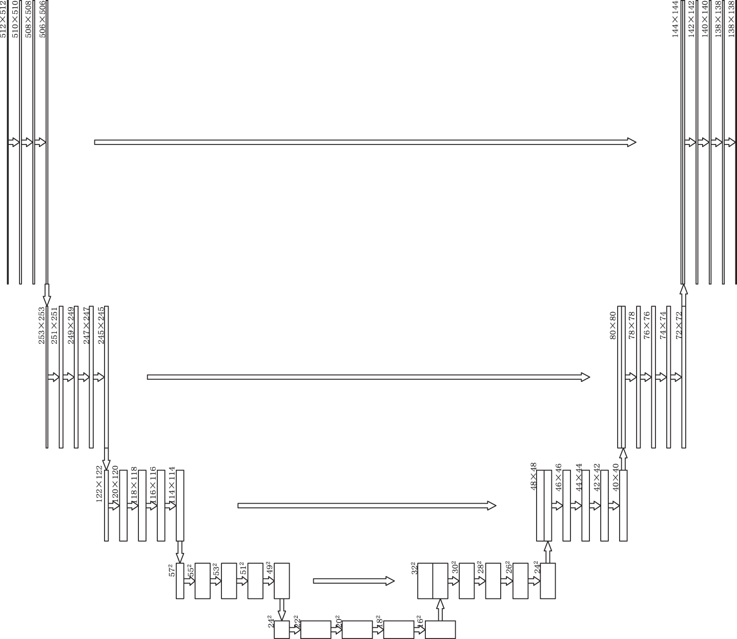
Improved U-net architecture.
Hyper-parameters of the experiments(U-net)
Next, we use three differently processed datasets to separately train the CNN model. In this experiment, we selected six representative CNN classification models for research. InceptionV3, Resnet50, NASnet, MobilenetV2, Densenet121 and Se-Resnet50 networks. The parameters are shown in Table 3.
Summary of the utilized architectures
Summary of the utilized architectures
According to the experimental control variable method, we set the same hyper-parameters for the six classification networks, as shown in Table 4.
Hyper-parameters of the experiments
We now briefly describe the characteristics of the six classification networks.
InceptionV3: the large convolutional block is decomposed into small convolutional blocks, the 7×7 convolutional block is decomposed into two 3×3 convolutional blocks, the 3×3 convolutional block is decomposed into 1×3 convolutional block and 3×1 convolutional block, and multiple convolutional blocks are used for parallel convolution. Then, channel dimensions are spliced to achieve the same effect as that when using a large convolutional block, and parameters are reduced; the structure is shown in Fig. 6 [17].
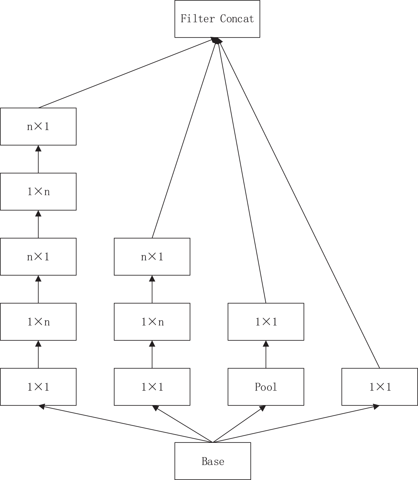
InceptionV3 structure.
Resnet50: a 1×1 convolutional block is used for dimensionality reduction in the residual term, and features are extracted through a 3×3 convolutional block, and finally a 1×1 convolutional block is used for dimensionality increase. The identity of the previous layer is also mapped and added to the residual term to obtain the output. The structure is shown in Fig. 7 [18].
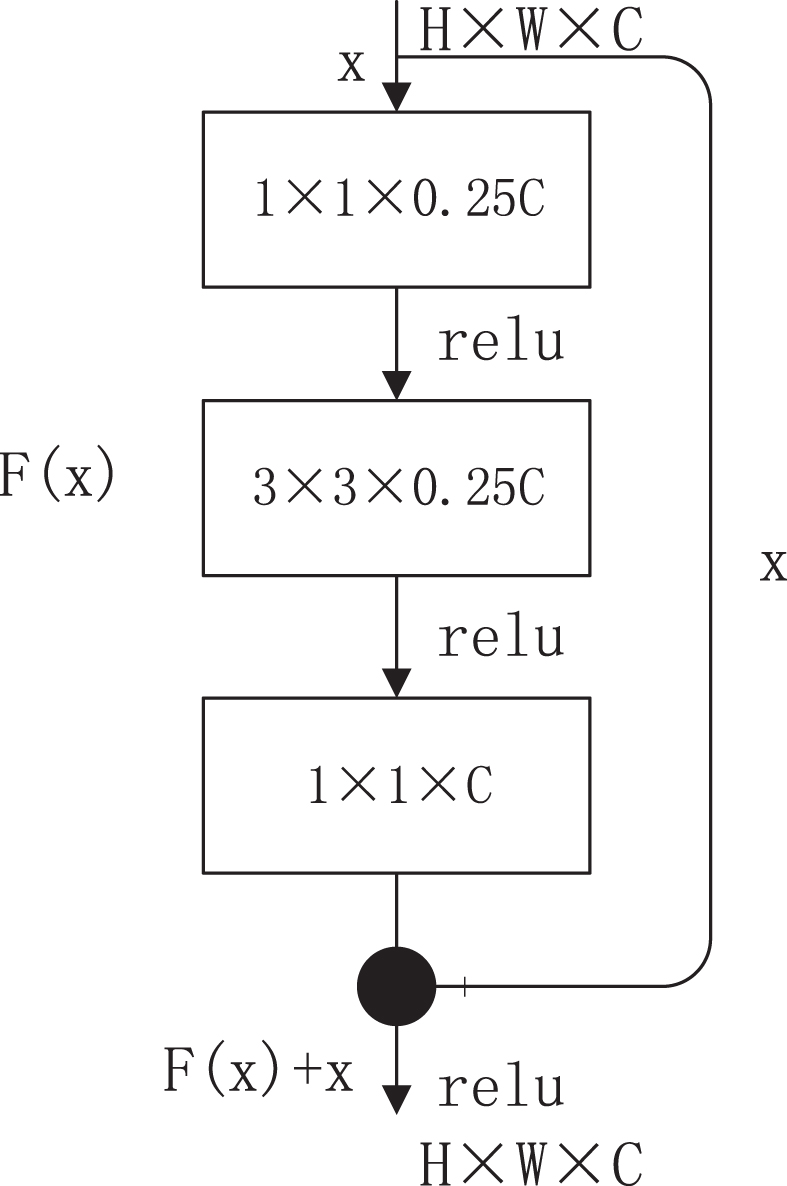
Resnet50 structure.
Densenet121: draws on the idea of the residual in Resnet50, and maps the output of each layer to the input of each subsequent layer. The structure is shown in Fig. 8 [19].

Densenet121 structure.
Se-Resnet50: Further improved on the basis of the residual structure in Resnet50, adding the squeeze and excitation blocks to make the network more nonlinear, better fit the complex correlation between channel performance, and greatly reduce the number of parameters and amount of calculations. Then, the normalized weight between 0 and 1 is obtained through a sigmoid gate, and a scale operation is used to weigh the normalized weight to the features of each channel. The structure is shown in Fig. 9 [20].
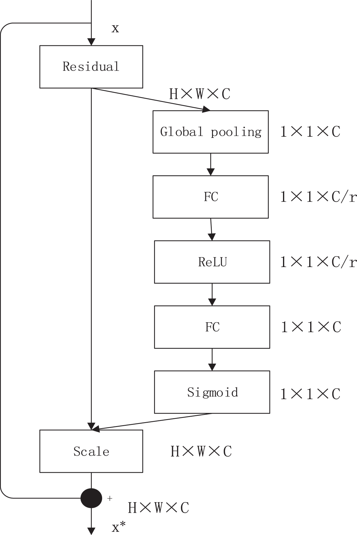
Se-resnet50 structure.
NASnet: Automatically trained using AutoML. The model performs a neural network architecture search on the dataset so that AutoML can find the best layer, flexibly stack multiple times to create the final network, and transfer the best learned architecture to image classification [21].
MobilenetV2: Its structure is similar to that of Resnet50, but unlike Resnet50, MobilenetV2 first performs dimensionality increase processing on the input, performs deep convolution (DW) on the dimensionality increase output, and then performs dimensionality reduction processing, that is, reverses the residual; the structure is shown in Fig. 10 [22].
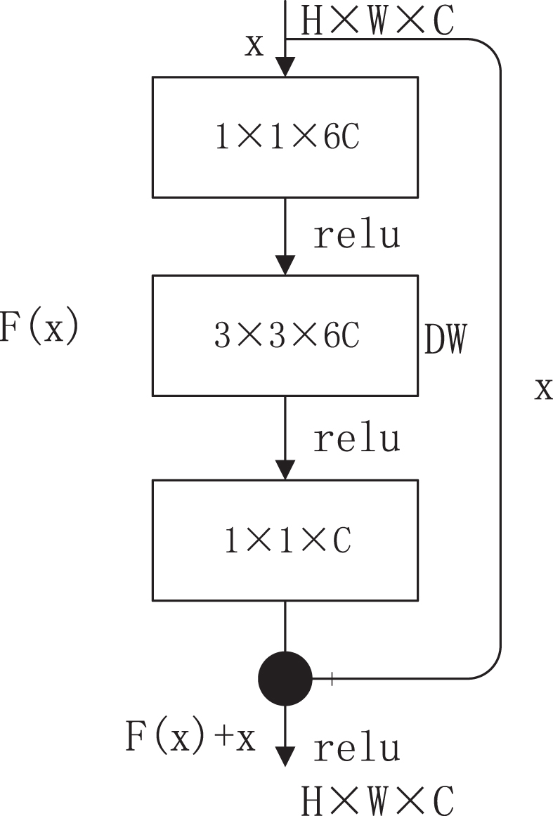
MobilenetV2 structure.
In this section, we used general multi-category evaluation indicators, namely, accuracy, recall, precision, and F1-score. These indicators are calculated by basic indicators, which are true positive(TP), false positive(FP), true negative(TN) and false negative(FN). TP predicts a positive class as a positive class, FP predicts a negative class as a positive class, TN predicts a negative class as a negative class, and FN predicts a positive class as a negative class.
Accuracy: The probability that the prediction is correct in the total sample. We used both the Top1 and Top2 accuracy rates.
Recall: The ratio of the number of retrieved related documents to the number of all related documents in the document library. It is also called recall rate or true rate.
Precision: describes the rate at which the prediction is correct when the prediction result is positive.
F1-score: the harmonic function of precision and recall.
Results
Because many calculations are required to train CNNs, all experiments were performed on a deep learning workstation. The workstation configuration is shown in Table 5. The training process was carried out in the PyTorch environment, and the programming language used Python 3.6.
Machine specifications
Machine specifications
In this experiment, we evaluated the accuracy, recall rate, precision rate, and F1-score of six CNN networks. The experiment results are shown in Table 6.
Performance measures (%) for every model
* Original U-net model segmentation, ** Improved U-net model segmentation.
All models showed similar and significant statistical performance. In all classification networks that used the improved U-net model to segment the dataset, the Top2 accuracy showed that the result of InceptionV3 was the best, reaching 97.7%. This was followed by Densenet121 and Resnet50, reaching 96.7% and 96.5%. The bottom three were MobilenetV2, Nasnet and Seresnet50, with Top2 accuracy rates of 94%, 92.7% and 92.2% respectively. In the classification network of all the datasets segmented by the original U-net model, the top three were Densenet121, Resnet50 and InceptionV3, and the bottom three were Nasnet, MobilenetV2 and Seresnet50. In all classification networks that were not segmented, the top three were still Resnet50, InceptionV3 and Densenet121, and the bottom three were still Nasnet, Seresnet50 and MobilenetV2.
On the other hand, the table shows that in each classification network, the Top2 accuracy of the classification network of the dataset segmented by the improved U-net is better than the classification of the dataset segmented by the original U-net. The network was better than the classification network of the undivided dataset. Moreover, the use of the U-net model for segmentation had different lifting effects on each classification network. In the four networks of Seresnet50, InceptionV3, Densenet121 and MobilenetV2, the improvement effect could reach about 3%. In Resnet50 and Nasnet, an increase of about 1% could also be achieved.
In addition, Table 7 shows the confusion matrix of the model based on performance metrics and the best results. On the basis of the results, the performance of the classifier could be intuitively evaluated, and the InceptionV3 model neurons using the improved U-net segmentation dataset could be used to determine which classes were highlighted. Rows are related to the output class, and columns are related to the true class. Diagonal cells are associated with correctly classified observations, and off-diagonal cells correspond to misclassified observations.
Confusion matrix based on InceptionV3 model. (1) black grass. (2) charlock. (3) cleavers. (4) common chickweed. (5) common wheat. (6) fat hen. (7) loose silky bent. (8) maize. (9) scentless mayweed. (10) shepherd purse. (11) small flowered cranesbill. (12) sugar beet
It is obvious from the confusion matrix in Table 7 that there were many misjudgments between black grass and loose silky bent. It recognized 19 pictures of black grass as loose silky bent, 11 pictures of loose silky bent were recognized as black grass, and the recognition accuracy of other types of plants was higher. In addition, we calculated the classification performance metric for each category, and the result of using the segmented InceptionV3 model is shown in Fig. 11.

Performance results for each class.
In addition, we compared the results with the work of other authors, as shown in Table 8, and our proposed method improved the performance of CNN to obtain better results.
Summary of techniques and comparison between studies for classification of plant diseases
The development of deep learning technology allows for using digital images to classify crops and weeds. When weeds are still in the seedling stage, we could establish a fast and accurate classification model to screen the weeds. The dataset that we used in this study was 3 crops and 9 weeds, with a total of 5519 pictures. We divided the dataset according to the ratio of 9:1, and performed three different segmentation operations on the training set. After training the six typical CNN classification models of Seresnet50, InceptionV3, Densenet121, Resnet50, Nasnet, and MobilenetV2, 18 classification results were obtained.
Among the six typical CNN models, the small networks Nasnet and MobilenetV2 showed poor Top2 accuracy on the three segmented datasets because of fewer parameters. Seresnet50, which had the largest parameter, had too many useless parameters on the three segmented datasets, resulting in a decrease in accuracy. In InceptionV3, Densenet121, and Resnet50, the parameters of InceptionV3 and Resnet50 were relatively close, and were significantly more than the parameters of Densenet121 were. However, in terms of Top2 accuracy, the values of InceptionV3, Resnet50 and Densenet121 were relatively close. This shows that, in the classification of plant seedlings, a model with appropriate parameters can achieve a better classification effect. When the two U-net models were introduced for segmentation, the accuracy of each classification network was significantly improved, and the Top2 accuracy increased from 1% to 4%. This shows that, if the U-net model is used to perform image processing, segmentation can improve the performance of the classification network. Moreover, using the improved U-net model for segmentation combined with the InceptionV3 classification network can achieve a Top2 accuracy rate of 97.7%.
All of the above classification models use different metrics to evaluate, including accuracy, recall, precision, and F1-score, and they all use the same hyperparameters. Table 6 shows that using the U-net segmentation model for segmentation with the InceptionV3 network model achieved better results than those of other combined models. Table 7 shows the confusion matrix of the classification results of the hybrid model using the improved U-net combined with InceptionV3. The confusion matrix showed that, since black grass and loose silky bent are very similar, the hybrid model had a high error rate in identifying them. As shown in Fig. 12, since these two types of plants are very similar in appearance, they cannot be distinguished by the naked eye. Therefore, the confusion matrix also showed that the classification network could not distinguish between black grass and loose silky bent. Since there were only 12 classified plant seedlings, if Top5 accuracy is used, even better results can be obtained, but the ability to distinguish crops is reduced. Moreover, in practical applications, these two types of plants are weeds, and failure to discriminate the seedlings of these two weeds does not affect the removal of weeds, so we used the Top2 accuracy rate as the evaluation standard of the CNN model.
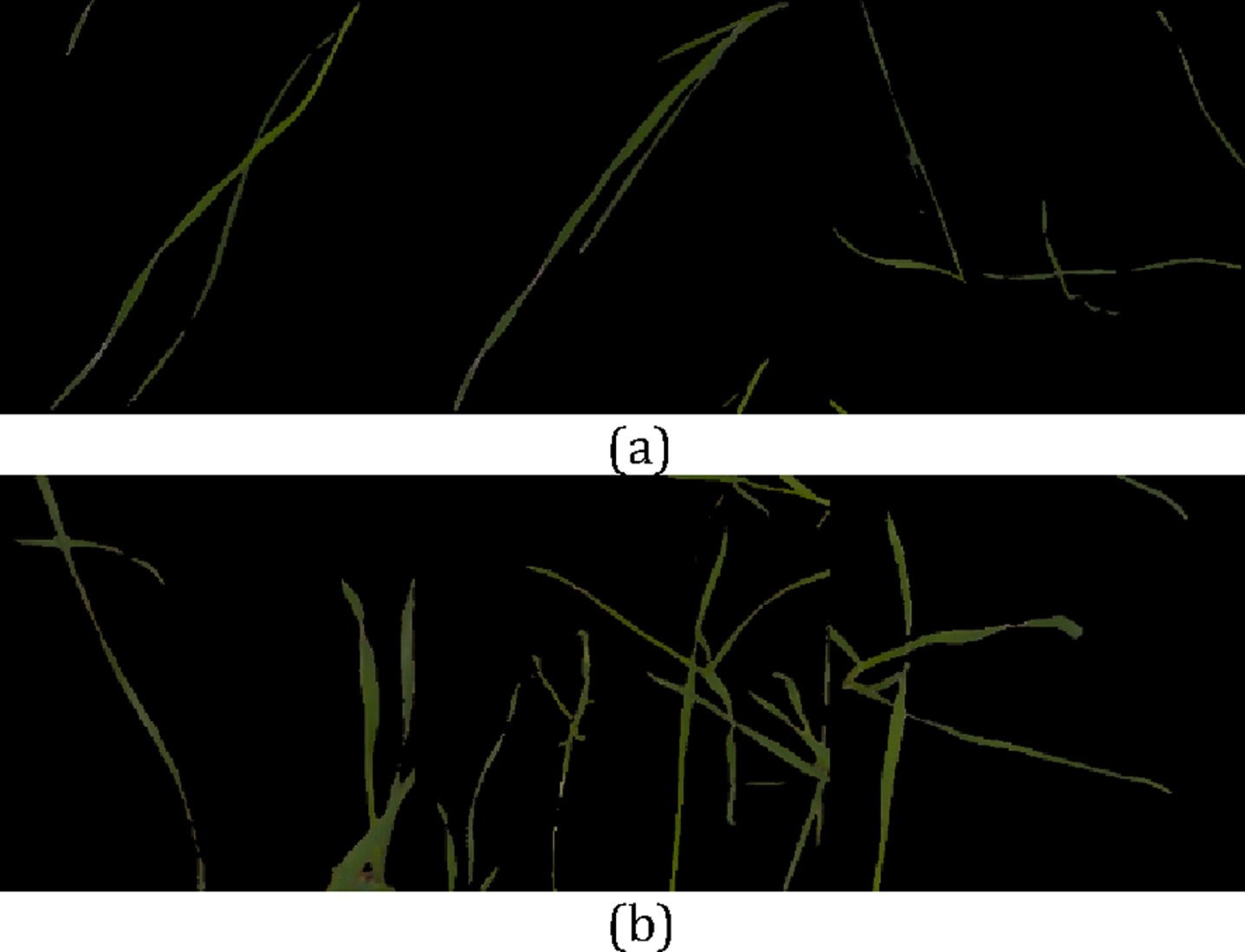
Test image. (a) Black Grass. (b) Loose Silky Bent.
On the other hand, this work has some limitations. We did not produce a more detailed distinction between black grass and loose silky bent in order to achieve more precise results, and the U-net model that is often used when processing medical images was used in the experiment for segmentation. This requires operators to understand the content of image segmentation and classification, which is not conducive to users or farmers with little or no professional knowledge.
This paper proposed a two-stage plant seedling classification method based on deep learning. We used the three processing methods of the improved U-Net, the original U-Net, and no segmentation for the dataset, and the six classification models of Seresnet50, InceptionV3, Densenet121, Resnet50, Nasnet, and MobilenetV2 for verification. Through experiments, after using the improved U-Net for image segmentation, better classification performance were achieved. Although each model used in this work could be classified from 3 crop seedlings and 9 weed seedlings, the improved U-Net combined with the InceptionV3 classification model proposed in this paper could achieve a Top2 accuracy rate of 97.7%. Its classification performance was the best, which is of great significance for the classification of plant seedlings.