A novel MapReduce-based deep convolutional neural network algorithm

Abstract

Deep convolutional neural networks (DCNNs), with their complex network structure and powerful feature learning and feature expression capabilities, have been remarkable successes in many large-scale recognition tasks. However, with the expectation of memory overhead and response time, along with the increasing scale of data, DCNN faces three non-rival challenges in a big data environment: excessive network parameters, slow convergence, and inefficient parallelism. To tackle these three problems, this paper develops a deep convolutional neural networks optimization algorithm (PDCNNO) in the MapReduce framework. The proposed method first pruned the network to obtain a compressed network in order to effectively reduce redundant parameters. Next, a conjugate gradient method based on modified secant equation (CGMSE) is developed in the Map phase to further accelerate the convergence of the network. Finally, a load balancing strategy based on regulate load rate (LBRLA) is proposed in the Reduce phase to quickly achieve equal grouping of data and thus improving the parallel performance of the system. We compared the PDCNNO algorithm with other algorithms on three datasets, including SVHN, EMNIST Digits, and ISLVRC2012. The experimental results show that our algorithm not only reduces the space and time overhead of network training but also obtains a well-performing speed-up ratio in a big data environment.

Keywords

DCNN MapReduce network compression conjugate gradient method load balancing

1 Introduction

The past decade has witnessed considerable progress in image recognition work with deep learning, which is based on structured deep neural networks [1 –3]. Deep convolutional neural network (DCNN) [4], one of the foremost families, embraces convolutional computation capable of downscaling a large number of parameters of an image and effectively preserving image features, which is virtually tailored for processing images. In particular, the advent of the big data era has opened the gateway for the rapid development of DCNNs. Many excellent deeper models have been proposed, the excellent AlexNet, VGG, GoogLeNet, ResNet and DenseNet [5 –9]. The learning of large amount of training data allows models to achieve better generalization ability and function approximation capability. However, with the exponential growth of data, several issues cannot be ignored. Most DCNNs use some convolutional layers in image recognition work before the fully connected layers. Convolutional layers aim to diminish image dimensionality, but they are computationally tedious and there may be invalid kernels in the convolutional kernel, which do not significantly help image classification results but incur significant inference costs. In this way, the network must be reconstructed and adapted to take into account solutions working in big data. One research direction is to remove redundancy by pruning. The general procedure is to measure the importance of neurons, remove some of the unimportant neurons, and fine-tune the network. In this way, by modifying the bulky model, it is possible to reduce its memory and time cost while obtaining as much performance as possible from its original unmodified model.

Backpropagation (BP) [10] is one of the most widespread supervised learning algorithms in multilayer feedforward neural networks. There are two weight update modes in the BP algorithm: online mode and batch mode. The batch update mode is more suitable for some popular frameworks that deal with big data (such as MapReduce [11]), because all items in the training set can be used simultaneously. Unfortunately, the original BP algorithm converges slowly when executing parameter updates and tends to fall into local optima, which seriously affects the training time. In addition, the stochastic gradient descent method [12] in BP algorithm involves a great deal of manual tuning to optimize the parameters when distributed or parallelized using clusters of computers. Compared to this, the conjugate gradient method [13] offers special features that allow the gradient computation to be distributed over different machines, while the training is more stable and the convergence is easier to check, but it is usually slower. Therefore, it is worth pondering how to accelerate the convergence of conjugate gradient method. On the other hand, the single machine training model requires high memory and time efficiency, and the parallelization within DCNN does not consider load balancing, which may result in long response time and inefficient parallelization. As one of the most popular Big Data frameworks, MapReduce provides new ideas for solving this problem. As one of the most popular Big Data frameworks, MapReduce provides a reliable, fault-tolerant and resilient computational framework for storing and processing large data sets that scales well as the size of the data set continues to grow. This definitely provides new ideas to improve the parallelization efficiency of DCNN.

Based on the above analysis, a new parallelized deep convolutional neural network algorithm combined with MapReduce is proposed. The experimental results indicate that the algorithm demonstrates excellent performance when dealing with large-scale datasets. And it works even better as the computing nodes grow. The main contributions of this study are as follows:

A feature map pruning (FMP) strategy was designed to effectively reduce redundant parameters.

A conjugate gradient method based on modified secant equation (CGMSE) is obtained in the map phase to achieve fast convergence of the conjugate gradient method.

To mitigate the effects of data skew in the reduce phase, a load balancing strategy based on regulate load rate (LBRLA) is developed to realize equal distribution of the data keys, thus ensuring the balance of computation completion time.

The rest of the paper is arranged as follows. Section 2 shows related work, and Section 3 introduces the DCNN and conjugate gradient methods. Then Section 4 describes the details of our proposed DCNN algorithm and analyzes its time complexity. After that, Section 5 shows our experimental design and comparison results; Finally, Section 6 concludes the paper.

2 Related Work

To assist readers, the relevant work mentioned in the manuscript is listed in Table 1. Substantial work has been done on reducing redundant parameters by pruning. Tung et al. [14] proposed the CLIP-Q method, which jointly performs weight pruning and weight quantification in parallel with fine-tuning. To some extent, it reduces the superfluous elements, but does not take into account the inter-layer differences in DCNN. Immediately afterwards, Lin et al. [15] combined two different regularizes for structured sparsity in the original filter pruning objective function to prune adaptively. By exerting structured sparsity and fully coordinating global output and local pruning operations, the number of filters and output feature mappings are simultaneously diminished, speeding up the computation. Unfortunately, this scheme is less efficient for pruning due to the structured sparsity that requires frequent access to memory. Yu et al. [16] assessed neuronal importance directly by back propagation weights. The importance-based criterion is extensively implemented for the purpose of reducing memory access. However, a drawback of this method is that its compression of high-dimensional information may degrade the accuracy.

Table 1
Literature merits and demerits

Literature Merits Demerits

[14] Joint weight pruning and weight quantification with fine-tuning Inter-layer differences in DCNN are ignored

[15] Combined two different structured sparse regularization methods for adaptive pruning Requires frequent memory access which makes pruning inefficient

[16] Implemented importance-based criteria, thus reducing memory access Compression of high-dimensional information may reduce accuracy

[17] Improved learning step-size and conjugate directions Gradient-dependent and time-consuming

[18] Both sufficient descent characteristics of the search direction and bounded characteristics of the spectral parameter sequence are guaranteed Without convexity of the objective function, it is not necessarily globally convergent.

[19] Globally convergent without the assumption of convexity of the objective function The direction of descent cannot be ensured and a restart may be required.

[20] A data-parallel strategy is used to divide the training samples to each computational node Model efficiency and loss of accuracy due to data separation are ignored

[21] Added elastic distortion to input data for improved accuracy Large amount of intermediate data is generated during the process, leading to frequent IO operations

[22] Local polymorphic parallel neural networks and many-to-many connections are designed to reduce the computational complexity Dependence on reliable performance indicators

[23] Combine with artificial bee colony method to find the optimal parameters in parallel, thus minimizing the classification error Low resource utilization due to insufficient utilization of the acceleration provided by parallelization and neglect of the server load capacity

Literature	Merits	Demerits
[14]	Joint weight pruning and weight quantification with fine-tuning	Inter-layer differences in DCNN are ignored
[15]	Combined two different structured sparse regularization methods for adaptive pruning	Requires frequent memory access which makes pruning inefficient
[16]	Implemented importance-based criteria, thus reducing memory access	Compression of high-dimensional information may reduce accuracy
[17]	Improved learning step-size and conjugate directions	Gradient-dependent and time-consuming
[18]	Both sufficient descent characteristics of the search direction and bounded characteristics of the spectral parameter sequence are guaranteed	Without convexity of the objective function, it is not necessarily globally convergent.
[19]	Globally convergent without the assumption of convexity of the objective function	The direction of descent cannot be ensured and a restart may be required.
[20]	A data-parallel strategy is used to divide the training samples to each computational node	Model efficiency and loss of accuracy due to data separation are ignored
[21]	Added elastic distortion to input data for improved accuracy	Large amount of intermediate data is generated during the process, leading to frequent IO operations
[22]	Local polymorphic parallel neural networks and many-to-many connections are designed to reduce the computational complexity	Dependence on reliable performance indicators
[23]	Combine with artificial bee colony method to find the optimal parameters in parallel, thus minimizing the classification error	Low resource utilization due to insufficient utilization of the acceleration provided by parallelization and neglect of the server load capacity

Aiming to accelerate the rate of convergence, a spectral conjugate gradient algorithm by modifying the learning step-size and conjugate directions is described in research [17], which only adopts the gradient direction for each line search and guarantees global convergence using a non-monotonic strategy. There is no free lunch, and its strong dependence on many functions and gradients predisposes it to be more time-consuming. Jian et al. [18] proposed a new spectral parameter generation method (JC method) with a step size obtained from a strong Wolfe or generalized Wolfe line search. By introducing a new double truncation technique, both the sufficient descent property of the search direction and the bounded property of the spectral parameter sequence can be guaranteed. The algorithm achieves global convergence for uniformly convex functions, but does not work for convexity without an objective function. As a modified version of the JC method, Faramarzi et al. [19] proposed a new spectral conjugate gradient method for unconstrained optimization problems and proved that it is globally convergent without the assumption of convexity of the objective function. Despite the success, all the above schemes pose restrictions, such as the inability to secure generation of descent directions, thus requiring the typically inefficient restart process to ensure convergence, which leads to potentially significant time consumption. Consequently, how to make the conjugate gradient method converge quickly is an urgent issue.

To date, many studies have tried to implement the convolution neural network by MapReduce. Zhao et al. [20] proposed the convolution neural network based on MapReduce (CNN-MR) algorithm, which adopts a data-parallel strategy to partition the training samples to each computational node. However, the method simply distributed the training samples without considering the efficiency of the model and the loss of accuracy due to data segregation. In [21], the MapReduce-based deep convolution neural network algorithm (MR-DCNN), developed by Basit et al. in 2017, added elastic distortion to the input data. Despite the improved accuracy, the algorithm struggles to achieve a satisfying balance between accuracy and computational cost. The large amount of intermediate data generated in the MapReduce process causes frequent IO operations, which will consume a lot of time. In the literature [22], the polymorphic parallel convolution neural network (PP-CNN) algorithm, developed by Zeng et al. in 2019, introduced deconvolution layer and designs local polymorphic parallel neural network and many-to-many connections. Their method reduces the computational complexity marginally, but it should be noted that it relies on reliable performance metrics, so availability is a limitation. To overcome these issues, Banharnsakun et al. [23] proposed a distributed artificial bee colony (distributed CNN-ABC) algorithm, which combined with the artificial bee colony method to find the optimal parameters in parallel, thereby minimizing classification errors and reducing time complexity. However, the above scheme failed to take full advantage of the acceleration provided by parallelization, and the non-uniform distribution of keys induce imbalance in task completion time and delay in the execution of the overall work, so how to design and implement an efficient parallel DCNN is still an urgent problem to be solved.

3 Preliminary

3.1 DCNN

DCNN extracts advanced semantic features of the image by utilizing multiple convolutional layers and pooling layers. It reduces the dimensionality of the feature map and preserves important feature information while ensuring image rotation invariance and translation invariance. Its training process is divided into two stages: forward propagation and back propagation.

During forward propagation process, the feature map is calculated for each layer input as $y_{l} = f (\sum_{r \in I} w_{r}^{l} * x_{r}^{(l - 1)} + b^{l})$ (1)

where * denotes a convolutional operation, y_l is the output of the lth convolutional layer, x^(l-1) and b^l are the input vector and the bias term of the l th layer. I is the set of input feature maps and f (x) is the activation function. The weights of the l th convolutional kernel of the rth level are denoted by I.

During back propagation process, let’s assume the dataset has M samples, and the forward propagation phase of the network will output predictions for each class by comparing the desired output of the network with the predicted outcome to adjust the weights. Define the final objective function of the network as $E (w) = min \sum_{i = 1}^{M} L (p_{r}) + λ (w)$ (2)

Here, L (p_r) is the loss function, and the classification error is reduced by iteratively training the network to reduce the loss function. p_r is the output of the last level in Equation (1), where it represents the input to the back propagation. λ (w) is the regularization function and w indicates the weight in the network.

3.2 Conjugate gradient method

Definition 2.1. The standard conjugate gradient method generates a sequence of weights {w_i} [24] using the following iterative formula: $w_{i + 1} = w_{i} + η_{i} d_{i}, i = 0, 1, . . ., N$ (3)

Here, i is the current iteration commonly denominated epoch, w₀ ∈ Rⁿ indicates a given initial point, η_i > 0 is the learning rate and d_i is the descent search direction.

Definition 2.2. In conjugate gradient method, the search direction [24] is the descent direction of the objective function value when searching for the optimal solution. That is, the negative gradient of the current iteration is linearly combined with the previous search direction, which is defined as Equation (4). $d_{u} = {\begin{matrix} - g_{0}, & i = 0 \\ - g_{i} + β_{i} d_{i - 1}, & otherwise \end{matrix}$ (4)

Use the following expressions to define the update parameter β_i [25, 26] in Equation (4): $β_{i}^{HS} = \frac{g_{i}^{T} y_{i - 1}}{y_{i - 1}^{T} d_{i - 1}}, β_{i}^{FR} = \frac{| | g_{i} | |^{2}}{| | g_{i - 1} | |^{2}}$ (5)

Here, g_i = ∇ E (w_i), y_i-1 = g_i - g_i-1, || · || represents the Euclidean norm.

Definition 2.3. The standard secant formula [27] is an approximate matrix expression of the Hesse matrix, namely $B_{i} s_{i - 1} = y_{i - 1}$ (6)

Definition 2.4. Modified secant formula (MS) [27] limits the gradient of the standard secant formula, thereby improving the curvature accuracy of the conjugate gradient method, defined as $B_{i - 1} s_{i - 1} = {\bar{y}}_{i - 1}, {\bar{y}}_{i - 1} = y_{i - 1} + \frac{θ_{i - 1}}{s_{i - 1}^{T} k} k$ (7) where k is arbitrary vector such that $s_{i - 1}^{T} k \neq 0$ , s_i-1 = w_i - w_i-1, θ_i-1 = 2 (E_i-1 - E_i) + (g_i + g_i-1) ^Ts_i-1.

Property 2.1. If s_i-1 satisfies constraints $s_{i - 1}^{T} (\nabla^{2} E_{i} s_{i - 1} - y_{i - 1}) = O (| | s_{k - 1} | |^{3})$ and $s_{i - 1}^{T} (\nabla^{2} E_{i} s_{i - 1} - {\bar{y}}_{i - 1})$ = O (||s_k-1||⁴), then the MS is more accurate as compared to the standard secant formula; if ||s_k-1||>1, then the standard secant formula is superior [27].

4 PDCNNO: Parallel Deep Convolutional Neural Networks Optimization Algorithm

In this section, we describe and analyze parallel deep convolutional neural networks optimization (PDCNNO) algorithm in detail. The structure of PDCNNO is shown in Fig. 1. Our algorithm has three kernels: model compression, obtaining local classification results, and obtaining global classification results. In the model compression phase, to achieve pruning of redundant parameters, the FMP strategy calculates the L_a-norm of the feature map to obtain the L_a-norm average of the convolutional kernel, and then pre-training the network to obtain the compressed model. In the phase of obtaining local classification results, the Split function is firstly applied to divide the entire dataset into file blocks of the same size and stored on each node; then CGMSE is used to update the parameters when a Map function is employed to train the network on each node. In the phase of obtaining global classification results, LBRLA is designed to improve the performance of the Reduce function in calculating the final weights of the network, so as to quickly obtain the global classification result.

Fig. 1

PDCNN algorithm structure.

4.1 Model compression

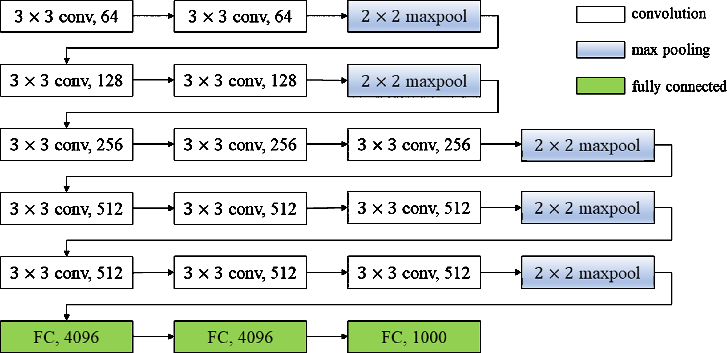
A DCNN usually contains many layers, each of which in turn contains many convolutional kernels. However, not all the weights in convolutional kernel are needed in predicting the network, so the network has a large number of redundant parameters. The traditional pruning method for redundant parameters is tocalculate the L₁-norm for each convolutional kernel. On this basis, convolutional kernels larger than the L₁-norm are considered significant, while those smaller than the L₁-norm are insignificant. In practice, the convolution kernel shows the features of a dimension of the image (e.g. outline, color), and it has degrees of depth. For example, the VGG16 configuration is shown in Fig. 2, which has 16 layers (13 convolutional and 3 fully connected layers), and its convolutional layers are divided into 5 segments, with a maximum pooling after each segment convolution. The 3 × 3 small convolution kernel is used to reduce the parameters and improve the fitting ability of the network. The 2 × 2 maximum pooling separates the layers from each other and the ReLU function is used for the activation units of all hidden layers. For shallower convolutional layers, it can only extract simple edges and color blocks. With conv1-1 (the first convolutional layer of VGG16), as shown in Fig. 3. (a), we can clearly see the outline of the whole bird, which is the edge feature of the object. Unlike shallower convolutional layers, deeper convolutional layers can focus on extracting highly abstract image features. As shown in Fig. 3. (b), conv4-1 (the eighth convolutional layer of VGG16) obtained high-level features such as the head, wings, and tail of the bird. ConsideringL₁-norm alone may face the problem of ignoring important convolutional kernels, so we proposed FMP to pre-train DCNN before using all the data for training.

Fig. 2

VGG16 Configuration.

Fig. 3

Feature map of (a) VGG16 conv1-1 and (b) VGG16 conv4-1 output.

The FMP first randomly selects some training data to pre-train the DCNN, and evaluates the importance of the convolutional kernel using the L_a-norm mean of the feature map. For each input sample x in the training dataset, the L_a-norm for the output of the convolution kernel can be computed, and then the mean value of the L_a-norm for all training samples is assigned to this kernel. The convolutional kernels are sorted by their corresponding mean values, and pruning is performed on those kernels having mean value less than a preset threshold. This pruning strategy can be repeated, recursively compressing the model and increasing computational speed.

Theorem 3.1. Suppose ||F_i,j||_a is the L_a-norm of the feature map F that corresponds to the output of the jth convolutional kernel when the ith sample is input to the network, and M is the number of samples randomly selected from the training data set. The formula for the L_a-norm is as Equation (8). ${\bar{La}}_{i} = \frac{\sum_{i = 1}^{M} | | F_{i, j} | |_{a}}{M}, a = {\begin{matrix} 1, low layer \\ \infty, deep layer \end{matrix}}$ (8)

Proof. Set the feature map of the output of the jth convolutional kernel as F_j at the ith sample input to the network. There are two cases. (1) If j ∈ low layer, then feature map F_j has a strong representation of semantic information but weak representation of geometric information, with a more homogeneous distribution of elements and many larger elements. (2) If j ∈ deep layer, then the feature map F_j has a strong representation of geometric details but weak representation of semantic information, with a concentrated distribution of elements and contains only a few larger elements. Therefore, for different levels of feature maps, distinct pruning methods should be applied. Owing to the properties of different norms (the L₁-norm will treat equally elements of different positions and sizes in the feature map, while the L_∞-norm will favor larger elements in the feature map), we can get: (1) if j ∈ low layer, we use the L₁-norm ( $| | X {| |}_{1} = \sum_{i = 1}^{n} | x_{i} |$ ) to prune in order to retain sufficient information for subsequent levels. (2) If j ∈ deep layer, we use the L_∞-norm (||X||_∞ = max(|x_i|)) for pruning, which screens out convolutional kernels containing larger elements.

Clearly, the use of FMP allows the removal of insignificant parameters and the retention of parameters that have an impact on the classification results. The pseudo code of model compression is shown in Algorithm 1.

Algorithm 1 The original database mining process
Input: partial data in the dataset DB.
Output: compressed sequence of DCNN weights
{w_m}.
1. for each sample∈ DB * x % do {
2. input DCNN for training neural network
3. for each convolution kernel do {
4. Get feature map (M, f)
5. ifM is low layer then
6. F_M = f₁
7. else F_M = \|\|f\|\|_∞
8. end if
9. end for
10. end for
11. for each m ∈ Mdo
12. La_m = avg (m, F)
13. sort (La_m)
14. for each La_mdo
15. del w_m which La_m < threshold (La_m)
16. end for
17. end for
18. output {w_m}

4.2 Obtaining local classification results

The obtaining of partial classification results includes Split phase and Map phase. During the Split phase, divides the original dataset into blocks of the same size using Hadoop’s default file block policy. During the Map phase, the Map function is used to calculate the local variation of each network weight parameter, and then the weights are updated to obtain local classification results. Since the stochastic gradient descent method of updating weights in Map phase is very slow to converge in a big data environment, this paper proposes CGMSE to search for the optimal parameters based on the quadratic convergence of the conjugate gradient method. There are three main steps to CGMSE, detailed below.

Step 1. Set the secant formula. Property 1 shows that the MS formula outperforms the standard secant formula if ${\bar{y}}_{i - 1}$ is more approximate to ∇²E_is_i-1 than y_i-1, but the opposite is true if ||s_k-1||>1. To overcome this shortcoming and improve the speed of the search, we propose an equilibrium secant formula. $B_{i - 1} s_{i - 1} = {\bar{y}}_{i - 1}, {\bar{y}}_{i - 1} = y_{i - 1} + σ_{i - 1} \frac{max {θ_{i - 1}, 0}}{s_{i - 1}^{T} k} k$ (9) where k is arbitrary vector such that $s_{i - 1}^{T} k \neq 0$ , s_i-1 = w_i - w_i-1, θ_i-1 = 2 (E_i-1 - E_i) + (g_i + g_i-1) ^Ts_i-1, w_i is the point at the i iteration, parameter σ_i-1 ∈ {0, 1}, σ_i-1 = 1 when s_i-1 ⩽ 1 and σ_i-1 = 0 otherwise.

Step 2. Set the parameters for the search direction. The search direction is the descent direction of the objective function value during the search for the optimal solution, and β_i is an important parameter that have impacts on the search direction. If β_i is not properly valued, it is quite likely that the conjugate gradient method will fail to find a convergent solution. Based on the global convergence principle of the conjugate gradient method [28], β_i is given as $β_{i}^{IHS} = max {\frac{g_{i}^{T} {\bar{y}}_{i - 1}}{{\bar{y}}_{i - 1} d_{i - 1}^{T}}, 0}$ (10)

Step 3. Set search direction. The conjugate gradient method for improved secant formulas does not ensure the generation of the descent direction, resulting in restarting the algorithm sometimes to ensure convergence. To avoid inefficient restarts, we set up Equation (11) based on the FR method [26] to solve for the search direction.

Theorem 3.2. Given $g_{i}^{T} d_{i} = - | | g_{i} | |^{2}$ , the search direction is as Equation (11). $d_{i} = - (1 + β_{i}^{IHS} \frac{g_{i}^{T} d_{i - 1}}{| | g_{i} | |}) g_{i} + β_{i}^{IHS} d_{i - 1}$ (11)

Proof Property 2.1 implies that Eq. (7) is more accurate than the standard secant formula when MS satisfies θ_i-1 = 2 (E_i-1 - E_i) + (g_i + g_i-1) ^Ts_i-1, $s_{i - 1}^{T} (\nabla^{2} E_{i} s_{i - 1} - y_{i - 1}) = O (| | s_{k - 1} | |^{3})$ , and $s_{i - 1}^{T} (\nabla^{2} E_{i} s_{i - 1} - {\bar{y}}_{i - 1}) = O (| | s_{k - 1} | |^{4})$ . So there is, if ||s_k-1||⩽1, ${\bar{y}}_{i - 1}$ is closer to ∇²E_is_i-1 than y_i-1, that is, Equation (7) is superior the standard secant formula β_is_i-1 = y_i-1. If s_k-1 > 1, β_is_i-1 = y_i-1 is superior to Equation (7). It follows that Equation (9) is the optimal solution, for all s_k-1 ∈ R. Thus, the convergence speed of CGMSE is greater than or equal to the other two methods (standard conjugate gradient method and conjugate gradient method with modification of the positive cut formula) in the real range.

The pseudo code for obtaining local classification results is shown in Algorithm 2.

Algorithm 2 Obtaining local classification results
Input: entire dataset D, initialization weights ω₀,
objective function E_G, maximum number
of iterations i_max.
Output: sequence of weights {w_i} of the network
in each node.
1. $E (w) = min \sum_{i = 1}^{M} L (p_{i}) + λ (w)$
2. $g_{i}^{T} d_{i} = - g_{i}^{2}$
3. ifE (w) ⩽ E_Gthen
4. output {w_i}
5. end if
6. ifg_i = 0 t hen
7. return “Mission Fail”
8. end if
9. update gradient by
$d_{k} = - (1 + β_{i}^{IHS} \frac{g_{i}^{T} d_{i - 1}}{g_{i}}) g_{i} + β_{i}^{IHS} d_{i - 1}$
10. calculate weight by Wolfe condition
11. $E (w_{k} + α_{k} d_{k}) - E (w_{k}) ⩽ ɛ_{1} α_{i} g_{i}^{T} d_{i}$ ,
$\| g {(w_{i} + α_{i} d_{i})}^{T} d_{i} \| ⩽ ɛ_{2} \| g_{i}^{T} d_{i} \|$
12. update weight w_i+1 = w_i + η_id_i
13. k = k + 1
14. ifi > i_maxt hen
15. return “Mission Fail”
16. else
17. goto step 2
18. end if

4.3 Obtaining global classification results

In the previous phase, each node is trained to obtain the local weights of DCNN. At this stage, the key-value pairs <key = (a, b) , value = w> output by each Map node are transmitted to the reduce function to complete the final merge and obtain the final network weights (w is the weight, and (a, b) is the bth weight of the ath convolutional kernel). Taking into consideration the impact of load balancing on the efficiency of parallel algorithms, this paper proposes LBRLA. It maintains load balancing and enhances system resource utilization through load distribution rules and setting load thresholds. The LBRLA is described below.

Given a server composed of nodes, where node S_i (i = 1, 2, . . . , n) has an inherent load of C_i and a current load of L_i, the following equation holds if the parallel system reaches load balancing. $P_{i} = \frac{L_{i}}{C_{i}} = \frac{L_{j}}{C_{j}}, i \neq jandi, j = 1, 2, \dots, n$ (12)

Here, P_i is the load rate of the ith node. Averaging the load rates of all nodes we get the current average load rate $\bar{P_{i}} = \frac{1}{n} \sum_{i = 1}^{n} P_{i}$ of the server. Theoretically, the load rate at each node should be equal to the average load rate when the server reaches load balancing, namely $\bar{P_{i}} = P_{1} = P_{2} = . . . = P_{n}$ (13)

However, according to fuzzy set theory [29], for each node of a parallel system, once the utilization of hardware resources (GPU, memory, network, disk) or parallel nodes exceed a certain percentage (such as 97%), the nodes can no longer handle the additional load. Accordingly, in the process of distributing load, it is necessary to evaluate the load by considering the following metrics: disk I/O usage, GPU usage, memory usage, network usage, parallel node usage, etc. Since they are all proportional to the load, we assign a weight to each metric, where disk I/O usage is D [i], GPU usage is G [i], memory usage is M [i], network usage is W [i], and node usage is N [i]. The combined node load rate is ${Load}_{i} = P_{i} (D [i] + G [i] + M [i] + W [i] + N [i])$ (14)

Then, in practice, when the server reaches load balancing, we have $\bar{Load} = {Load}_{1} = {Load}_{2} = . . . = {Load}_{n}$ (15)

The parallel system calculates the difference between the average load and the load per node; the larger the difference, the smaller the node load and the higher the priority of the node to allocate the load; similarly, the smaller the difference, the larger the node load and the lower the priority of the node to allocate the load. Since the MapReduce chunking mechanism makes it difficult to get each node load exactly the same, when the node load reaches $(1 - x %) \bar{{Load}_{i}}$ (x is an adaptive factor that can be set as needed), the parallel system will no longer allocate load to that node.

In summary, LBRLA takes into account parallel node load rate and load weight as metrics based on real-time feedback from parallel nodes. By controlling the load rate, the data volume and distribution of each node is more balanced. It not only ensures the load balance of each compute node, but also enhances and upgrades the resource utilization of the parallel system.

The pseudo code for obtaining the global classification results is shown in Algorithm 3.

Algorithm 3 Obtaining global classification results
Input: sequence of network weights {w_m} for each
compute node (m is the number of
weights in each network), initial number
of server nodes n, the intrinsic load of
node S_i (i = 1, 2, . . . , n) is C_i, the current
node load rate is P_i, and the number of
data blocks is N
Output: sequence of final network weights {w_m}
1. {w_m } = w₁, w₂, . . . , w_m
2. for each reduceNode do
3. Load_i = P_i (D [i] + G [i] + M [i] + W [i] + N [i])
4. if ${Load}_{i} < \bar{Load}$ then
5 loadList.append( $\bar{Load} - {Load}_{i}$ )
6. end if
7. sort(loadList)
8. end for
9. for each (a, b)∈ 〈 (a, b) , w_m 〉 d o
10. MapReduce.Reduce ((a, b) , w_m)
11. W_m = avg (w_m) which key=(a, b)
12. end for
13. output {W_m}

4.4 Time complexity

The time complexity of the PDCNNO algorithm is shown in Table 2 and it consists of the following three stage:

Model compression stage: assume the network contains D convolutional layers, C_l represents the number of convolutional cores in the lth convolutional layer, and M is the number of convolutional cores in each layer. The edge lengths of the output feature maps of the convolutional kernels, K represents the edge length of each convolutional kernel, and the number of pre-trained samples is m. Then the time complexity of the model compression using FMP is the sum of the feature map ordering time and the pruning time below the preset threshold weights, namely O (m log m) + O (m).

The stage of obtaining local classification results: suppose the number of Map nodes is a. Since each iteration of the CGMSE requires a matrix-vector multiplication and some vector inner product calculations, the complexity is O (n³) after completing n iterations. Therefore, the time complexity of obtaining local classification results is $O (\sum_{τ = 1}^{a} n^{3})$ .

The stage of obtaining global classification results: Assuming that the number of Reduce nodes is r, the time complexity of obtaining global classification results in Reduce stage is the quotient of the number of nodes and the total number of samples b, that is, O (b/r).

Table 2
Time complexity

Time complexity

Model compression O (m log m) + O (m)

Obtaining local classification results $O (\sum_{τ = 1}^{a} n^{3})$

Obtaining global classification results O (b/r)

PDCNNO $O (m (log m + 1) + b / r + \sum_{τ = 1}^{a} n^{3})$

	Time complexity
Model compression	O (m log m) + O (m)
Obtaining local classification results	$O (\sum_{τ = 1}^{a} n^{3})$
Obtaining global classification results	O (b/r)
PDCNNO	$O (m (log m + 1) + b / r + \sum_{τ = 1}^{a} n^{3})$

In conclusion, the time complexity of the PDCNNO algorithm is the sum of the above three stages, namely $O (m (log m + 1) + b / r + \sum_{τ = 1}^{a} n^{3})$ .

5 Experimental evaluation

In this section, we discuss the experimental setup, the experimental results and the corresponding analysis.

5.1 Experimental setup

We used the following three real datasets:

The SVHN [30] dataset contains color digital images from the real world, 32 × 32 pixels in size. The official dataset has 73257 images in the training set, 26,032 images in the test set, and 531,131 images for additional training. We segmented 6,000 images from the training set as a validation set and divided the pixel values by the 255, so their size is in the range [0,1], instead of using additional training images.

The EMNIST Digits [31] dataset is all black and white images of 32 × 32 pixels. It provides a handwritten digital dataset that is directly compatible with the original MNIST dataset. The dataset has a total of 280,000 images, including 240,000 images for the training set and 40,000 images for the test set.

The ISLVRC2012 [32] dataset contains 1,000 classes with 1,281,167 training images, 50,000 validation images, and 100,000 test images, each with multiple bounding boxes and corresponding class labels, and the entire dataset is approximately 150 G. Due to the inconsistency in image size, we cropped and scaled the images in the dataset to 224 × 224 and randomly selected 500 of these classes for the experiment.

Specific information about the dataset is shown in Table 3.

Table 3
Experimental datasets

SVHN EMNIST Digits ISLVRC2012

Number of images 73257 280000 612327

Image size 32 × 32 32 × 32 224 × 224

Dataset size 716 1228.8 68720

Number of classes 10 10 500

	SVHN	EMNIST Digits	ISLVRC2012
Number of images	73257	280000	612327
Image size	32 × 32	32 × 32	224 × 224
Dataset size	716	1228.8	68720
Number of classes	10	10	500

For the experimental hardware, we used 1 JobTracker node and 7 TaskTracker nodes. All nodes have an AMD Ryzen 7 CPU, 16GB RAM, with 8 processing units, a GPU of NVIDIA RTX2070 8 G, connected via 1Gb/s Ethernet. For software, the operating system installed in each node is Ubuntu 18.04, the MapReduce architecture is Apache Hadoop 2.7.4, and the software programming environment is java JDK 1.8.0. The specific configuration of the nodes is shown in Table 4.

Table 4

The foundation configuration of each node in the experiment

Node type	Host name	IP	Role
Master	Master	192.168.1.103	Master/JobTracker/NameNode
Slaver	Slaver_1∼Slaver_7	192.168.1.104∼192.168.1.110	Slaver/TaskTracker/DataNode

5.2 Experimental results and analysis

To validate the performance of the PDCNNO algorithm, we conducted experimental comparisons by evaluating the algorithm running time, memory usage, and speed-up ratio.

5.2.1 Running time and memory usage

We perform experiments based on the SVHN, EMNIST Digits, ISLVRC2012 dataset to comprehensively compare the PDCNNO algorithm with the MR-DCNN [21] algorithm, PP-CNN [22] algorithm, distributed CNN-ABC [23] algorithm, and a variant of the PDCNNO algorithm without model compression (denoted by PDCNN below). The running time and memory usage of the five algorithms are shown in Fig. 4.

Fig. 4

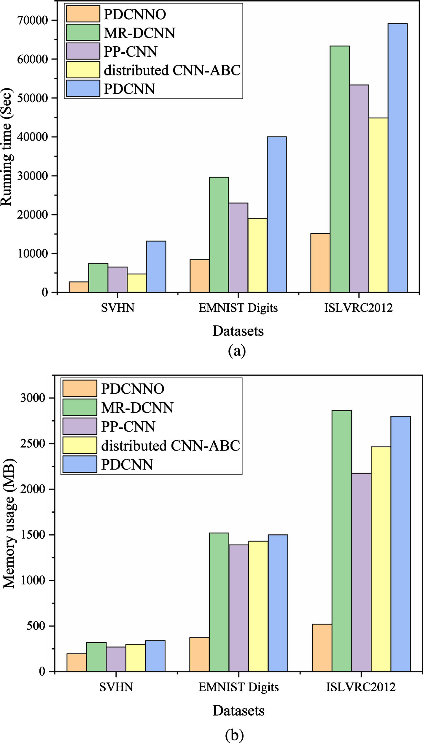
Comparison of (a) running time and (b) memory usage of each algorithm.

As shown in Fig. 4(a), the running time of the PDCNNO algorithm when processing the SVHN dataset is 36.31% of MR-DCNN, 41.25% of PP-CNN, 61.83% of distributed CNN-ABC, and 20.42% of PDCNN, respectively. Note that as the volume of data increases, the PDCNNO running time grows gently, while the other algorithms (including the PDCNN algorithm) increase geometrically. Especially when dealing with the largest dataset ISLVRC2012, the running time of the PDCNNO algorithm is 23.87% of MR-DCNN, 28.34% of PP-CNN, 41.47% of distributed CNN-ABC and 21.96% of PDCNN algorithm, respectively. The PDCNNO algorithm performs the best, while the ABC algorithm performs the second best. On the whole, there are three reasons for this result: firstly, since the pre-training time is much less relative to the algorithm running time, it has little impact on the overall performance of the PDCNNO algorithm; secondly, the distributed CNN-ABC algorithm manages to find the optimal initial weights, which improves time efficiency to some extent, but pruning of the network method in this study, directly led to a low-complexity network that accelerated model operation; finally, the use of CGMSE speeds up network convergence, thereby reducing running time better.

From a memory usage perspective (as shown in Fig. 4(b)), when processing the SVHN dataset, our algorithm is 53.23% of MR-DCNN,72.7% of PP-CNN, 57.65% of the distributed CNN-ABC and 57.65% of PDCNN, respectively. The superiority of the PDCNNO algorithm is becoming apparent when processing the latter two datasets. It can be noticed that the memory usage of the PDCNNO changes slightly, while the memory usage of the remaining algorithms increases sharply with larger datasets. Focusing on the comparison of the four algorithms it is revealed that they differ little on the first two datasets, except that the PP-CNN and distributed CNN-ABC algorithms perform slightly better on the dataset ISLVRC2012. This is attributed to the many-to-many connections used by the PP-CNN algorithm to guarantee continuous memory in the model. The more acceptable memory usage of the PDCNNO algorithm comes mainly from its pruning strategy. By pruning the redundant parameters via FMP, the number of parameters is substantially reduced, with a consequent reduction in running time and memory usage. Therefore, it can be concluded that the PDCNNO algorithm can significantly improve the training efficiency of DCNN in a big data environment and ensure the efficient operation of the model.

5.2.2 Speed-up ratio

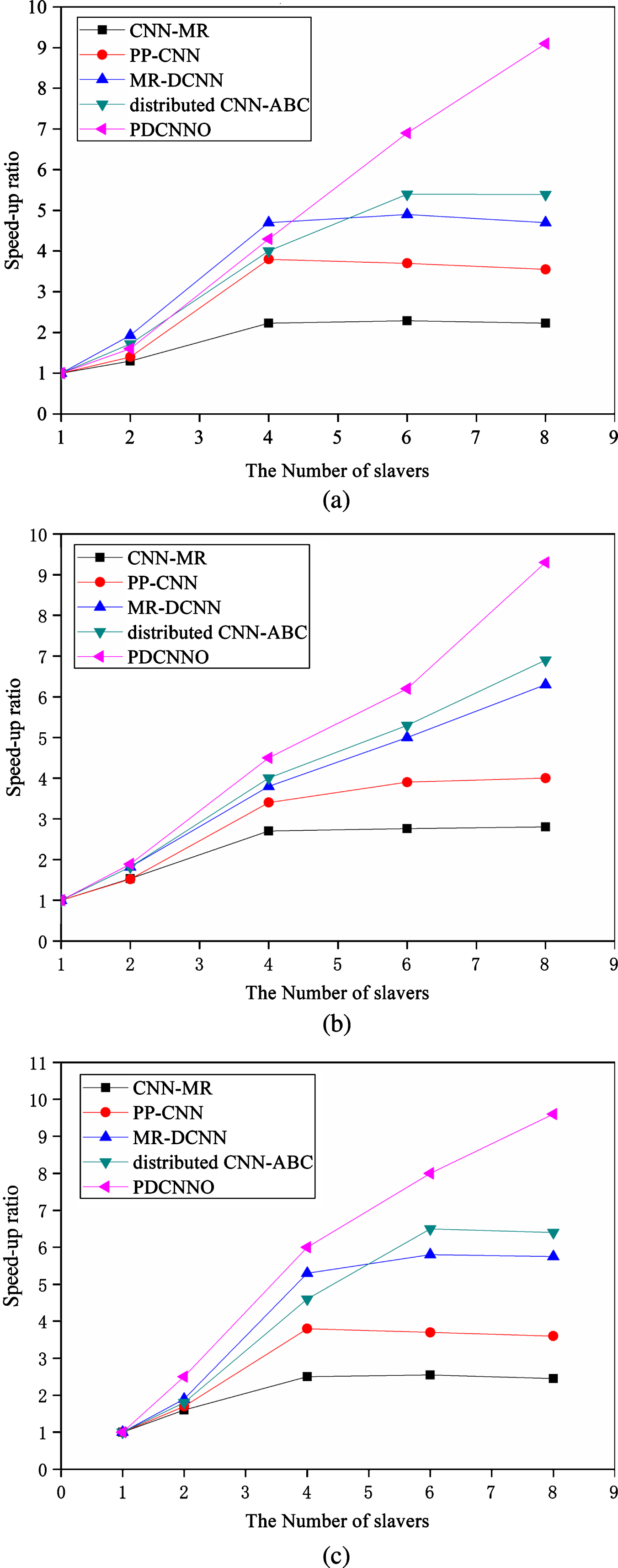
Speed-up ratio is typically used as a significant indicator to measure the parallelization performance of the algorithm. The speed-up ratio refers to the ratio of time, which is defined as $Speedup = \frac{T_{s}}{T_{p}}$ where T_s and T_p denote the running time of the algorithm in serial and in parallel, respectively. Figure 5 compares experimentally the speed-up ratios of PDCNNO and four algorithms, namely CNN-MR [22], MR-DCNN [23], PP-CNN [24] and distributed CNN-ABC [25], using data sets of different scales.

Fig. 5

Speed-up ratios for each algorithm on (a) SVHN, (b) EMNIST Digits and (c) ISLVRC2012.

From Fig. 5, it can be seen that the speed-up ratio of each algorithm follows an increasing trend with the number of nodes. When the number of nodes is small, such as 2, the difference among the algorithms’ speed-up ratios on the three datasets is not significant, although the value is slightly larger using the ISLVRC2012 dataset. In other words, with fewer nodes, the PDCNNO algorithm incurs time overhead in cluster operation, task scheduling, node storage, and other aspects, which slow down the computation speed of the algorithm, so the parallel performance of the PDCNNO algorithm is not good in this case. However, as the number of nodes increases to 6, the speed-up ratio of the PDCNNO algorithm surpasses other algorithms, for instance, it is higher than the MR-DCNN, distributed CNN-ABC, PP-CNN, and CNN-MR algorithms by 2.0, 1.5, 3.2, and 3.9, using SVHN dataset. This difference becomes more pronounced with rising number of nodes, and as we see from the different datasets, the speed-up ratios of the four comparison algorithms eventually stabilize, whereas the speed-up ratios of the PDCNNO algorithm essentially increase linearly with increasing number of nodes. This is due to the fact that the PDCNNO algorithm distributes the classification results equally among the computing nodes using LBRLA, and the advantage of the algorithm to compute the classification results and update the weights in parallel is gradually amplified. From Fig. 5(c), we observe that the acceleration ratio of PDCNNO is consistently better than the other algorithms. This result further suggests that the PDCNNO algorithm is suitable for processing larger datasets, and the parallel performance of the algorithm is greatly improved while the number of computational nodes is increased.

6 Conclusions

To compensate for the shortcomings of the traditional DCNN algorithm in terms of redundant parameters, slow convergence, and inefficient parallel performance in a big data environment, this research proposes the PDCNNO algorithm and provides an in-depth exploration and evaluation of its parallel design and implementation. At first, pre-training a portion of the randomly selected data and designing an FMP to reduce redundant parameters in the network by comparing the average value of L_a-norm. Next, we trained the network using the MapReduce model and propose CGMSE during parameter updates in the Map phase, which accelerates convergence by optimizing the search direction. Finally, we presented LBRLA in the Reduce phase to solve the problem of load imbalance across nodes in parallel systems and improve the parallel performance of the algorithm. Furthermore, in our experiments, the proposed algorithm and other techniques are compared in detail, including CNN-MR algorithm, MR-DCNN algorithm, PP-CNN algorithm, distributed CNN-ABC algorithm and PDCNN algorithm. Experimental results illustrated that our algorithm significantly outperforms the other compared algorithms in terms of running time, memory usage and speed-up ratio. And for larger datasets, the PDCNNO algorithm is more adaptable.

However, there remains room for improvement of the algorithm. For instance, pruning is limited by the width of the convolutional layer and the threshold for evaluating the L_a-norm needs to be adjusted manually. A future effort is to design an adaptive pruning so that the parameters can be applied to more general cases. Moreover, another point to note is that the algorithm provides insignificant performance improvement or even performance drops when dealing with small data sets. As such, it will be our direction to explore in the future by further improving the resource utilization of Hadoop clusters.

References

Islam

M.T.

, Siddique

B.M.N.K.

, Rahman

and Jabid

, Image recognition with deep learning, International Conference on Intelligent Informatics and Biomedical Sciences 3 (2018), 106–110.

Traore

B.B.

, Kamsu-Foguem

and Tangara

, Deep convolution neural network for image recognition, Ecological Informatics 48 (2018), 257–268.

Dourado

C.M.

, Da Silva

S.P.P.

, Da Nóbrega

R.V.M.

, Rebouças Filho

P.P.

, Muhammad

and De Albuquerque

V.H.C.

, An open IoHT-based deep learning framework for online medical image recognition, IEEE Journal on Selected Areas in Communications 39(2) (2020), 541–548.

Zhou

D.X.

, Theory of deep convolutional neural networks: Downsampling, Neural Networks 124 (2020), 319–327.

Shanthi

and Sabeenian

R.S.

, Modified Alexnet architecture for classification of diabetic retinopathy images, Computers & Electrical Engineering 76 (2019), 56–64.

Alippi

, Disabato

and Roveri

, Moving convolutional neural networks to embedded systems: the alexnet and VGG-16 case, IEEE International Conference on Information Processing in Sensor Networks (2018), 212–223.

Khan

R.U.

, Zhang

and Kumar

, Analysis of ResNet and GoogleNet models for malware detection, Journal of Computer Virology and Hacking Techniques 15(1) (2019), 29–37.

Wang

, Jia

, Lu

and Xia

, Thorax-Net: an attention regularized deep neural network for classification of thoracic disease on chest radiography, IEEE Journal of Biomedical and Health Informatics 24(2) (2020), 475–485.

Han

, Li

and Wang

, Channel-attention-based DenseNet network for remote sensing image scene classification, IEEE Journal of Selected Topics in Applied Earth Observations and Remote Sensing 13 (2020), 4121–4132.

10.

Lillicrap

T.P.

, Santoro

, Marris

, Akerman

C.J.

and Hinton

, Backpropagation and the brain, Nature Reviews Neuroscience 21(6) (2020), 335–346.

11.

Verma

, Malhotra

and Singh

, Big data analytics for retail industry using MapReduce-Apriori framework, Journal of Management Analytics 7(3) (2020), 424–442.

12.

Xie

, Wu

and Ward

, Linear convergence of adaptive stochastic gradient descent, International Conference on Artificial Intelligence and Statistics (2020), 1475–1485.

13.

Malik

, Mamat

and Abas

S.S.

, Convergence analysis of a new coefficient conjugate gradient method under exact line search, International Journal of Advanced Science and Technology 29(5) (2020), 187–198.

14.

Tung

and Mori

, Deep neural network compression by in-parallel pruning-quantization, IEEE Transactions on Pattern Analysis and Machine Intelligence 42(3) (2020), 568–579.

15.

Lin

, Ji

, Li

, Deng

and Li

, Toward compact convNets via structure-sparsity regularized filter pruning, IEEE Transactions on Neural Networks and Learning Systems 31(2) (2020), 574–588.

16.

, Li

, Chen

C.F.

, Lai

J.H.

, Morariu

V.I.

, Han

, Gao

, Lin

C.Y.

and Davis

L.S.

, NISP: Pruning networks using neuron importance score propagation, Proceedings of the IEEE Conference on Computer Vision and Pattern Recognition, (2018), 9194–9203.

17.

Birgin

E.G.

and Martínez.

J.M.

, A spectral conjugate gradient method for unconstrained optimization, Journal of Yulin Normal University 43 (2016), 117–128.

18.

Jian

, Chen

, Jiang

, Zeng

and Yin

, A new spectral conjugate gradient method for large-scale unconstrained optimization, Optimization Methods and Software 32(3) (2017), 503–215.

19.

Faramarzi

and Amini

, A modified spectral conjugate gradient method with global convergence, Journal of Optimization Theory and Applications 182(2) (2019), 667–690.

20.

Zhao

, Dong

, Ota

, Wu

, Li

and Li

, MapReduce enabling content analysis architecture for information-centric networks using CNN, IEEE International Conference on Communications (2018), 1–6.

21.

Basit

, Zhang

, Wu

, Liu

, Bin

, He

and Hendawi

A.M.

, MapReduce-based deep learning with handwritten digit recognition case study, IEEE International Conference on Big Data (2017), 1690–1699.

22.

Zeng

, Ding

and Jia

, Single image super-resolution using a polymorphic parallel CNN, Applied Intelligence 49(2019), 292–300.

23.

Banharnsakun

, Towards improving the convolutional neural networks for deep learning using the distributed artificial bee colony method, International journal of machine learning and cybernetics 10 (2019), 1301–1311.

24.

Zou

, Xia

and Cao

, Dense Broad Learning System based on Conjugate Gradient, International Joint Conference on Neural Networks (2020), 1–6.

25.

, Wu

and Yuan

, Some modified Hestenes-Stiefel conjugate gradient algorithms with application in image restoration, Applied Numerical Mathematics 158(2020), 360–376.

26.

Sun

, Liu

and Wang

, Two improved conjugate gradient methods with application in compressive sensing and motion control, Mathematical Problems in Engineering, (2020).

27.

Boutet

, Haelterman

and Degroote

, Secant Update generalized version of PSB: a new approach, Computational Optimization and Applications 78(3) (2021), 953–982.

28.

Jiang

and Jian

, Improved Fletcher–Reeves and Dai–Yuan conjugate gradient methods with the strong Wolfe line search, Journal of Computational and Applied Mathematics 348(2019), 525–534.

29.

Khorasani

E.S.

, Cremeens

and Zhao

, Implementation of scalable fuzzy relational operations in MapReduce, Soft Computing 22(9) (2018), 3061–3075.

30.

Yuan

and He

, Ensemble Generative Cleaning with Feedback Loops for Defending Adversarial Attacks, Proceedings of the IEEE/CVF Conference on Computer Vision and Pattern Recognition (2020), 581–590.

31.

Cohen

, Afshar

, Tapson

and Schaik

, EMNIST: Extending of MNIST to handwritten letters, 2017 International Joint Conference on Neural Networks (2017), 2161–4407.

32.

Krizhevsky

, Sutskever

and Hinton

G.E.

, Imagenet classification with deep convolutional neural networks, Advances in Neural Information Processing Systems 25 (2012), 1097–1105.

A novel MapReduce-based deep convolutional neural network algorithm

Abstract

Keywords

1 Introduction

2 Related Work

3.1 DCNN

Table 2 Time complexity Time complexity Model compression O (m log m) + O (m) Obtaining local classification results O ( ∑ τ = 1 a n 3 ) Obtaining global classification results O (b/r) PDCNNO O ( m ( log m + 1 ) + b / r + ∑ τ = 1 a n 3 )

5.1 Experimental setup

Table 3 Experimental datasets SVHN EMNIST Digits ISLVRC2012 Number of images 73257 280000 612327 Image size 32 × 32 32 × 32 224 × 224 Dataset size 716 1228.8 68720 Number of classes 10 10 500

5.2.1 Running time and memory usage

References

Table 2
Time complexity

Time complexity

Model compression O (m log m) + O (m)

Obtaining local classification results $O (\sum_{τ = 1}^{a} n^{3})$

Obtaining global classification results O (b/r)

PDCNNO $O (m (log m + 1) + b / r + \sum_{τ = 1}^{a} n^{3})$

Table 3
Experimental datasets

SVHN EMNIST Digits ISLVRC2012

Number of images 73257 280000 612327

Image size 32 × 32 32 × 32 224 × 224

Dataset size 716 1228.8 68720

Number of classes 10 10 500