An adaptive forecast combination approach based on meta intuitionistic fuzzy functions

Abstract

Intuitionistic meta fuzzy forecast combination functions are introduced in the paper. There are two challenges in the forecast combination literature, determining the optimum weights and the methods to combine. Although there are a few studies on determining the methods, there are numerous studies on determining the optimum weights of the forecasting methods. In this sense, the questions like “What methods should we choose in the combination?” and “What combination function or the weights should we choose for the methods” are handled in the proposed method. Thus, the first two contributions that the paper aims to propose are to obtain the optimum weights and the proper forecasting methods in combination functions by employing meta fuzzy functions (MFFs). MFFs are recently introduced for aggregating different methods on a specific topic. Although meta-analysis aims to combine the findings of different primary studies, MFFs aim to aggregate different methods based on their performances on a specific topic. Thus, forecasting is selected as the specific topic to propose a novel forecast combination approach inspired by MFFs in this study. Another contribution of the paper is to improve the performance of MFFs by employing intuitionistic fuzzy c-means. 14 meteorological datasets are used to evaluate the performance of the proposed method. Results showed that the proposed method can be a handy tool for dealing with forecasting problems. The outstanding performance of the proposed method is verified in terms of RMSE and MAPE.

Keywords

Forecast combination meta-analysis intuitionistic fuzzy c-means meta fuzzy functions meteorology

1 Introduction

The concept of forecasting is defined as a planning tool for the future trends based mainly on data that were previously collected. Therefore, forecasting methods have been commonly used in variety fields, such as economics, meteorology, health sciences, consumption in all areas, and etc. Because the complex structure of a time series in real-life problems, there are hundreds of thousands forecasting methods in the literature that were proposed under different circumstances. While some of these methods are probabilistic, some of them are non-probabilistic. However, usually real-life time series datasets contain both probabilistic and non-probabilistic parts in them.

Probabilistic approaches have been introduced under strict assumptions, i.e. stationarity. Stationarity which requires that a time series dataset has a constant mean and covariance function is a strong assumption. Autoregressive Integrated Moving Average (ARIMA), which was organized by Box and Jenkins [19] to obtain the best ARIMA model parameters, is one of the most used traditional time series forecasting methods in probabilistic approaches. However, ARIMA models assume that there is a linear relationship between data. Because this is usually not the case in real life datasets, many researchers have studied alternative (non-probabilistic) methods for forecasting, such as Artificial Neural Networks (ANN), Fuzzy Inference Systems (FIS), and Fuzzy Time Series (FTS).

The first ANN method was proposed by McCulloch and Pitts [58]. It has been commonly studied topic by then. Recently, ANN method has been widely used for forecasting problems. Zhang [20] hybridized ARIMA and ANN in their studies. Yolcu et al. [54] took in consideration both linear and non-linear parts of a time series in their proposed ANN method. Gundogdu et al. [40] proposed multiplicative ANN based on Gaussian activation function. Li and Chan [44] proposed predictive time series modeling by adapting ANNs. Egrioglu et al. [15] introduced recurrent multiplicative neural network for non-linear time series forecasting. Khosravi et al. [1] used ANNs and support vector machines to predict wind speed and wind direction. Because, ANN based forecasting methods contribute the literature, multilayer perceptron ANN is included as a forecasting method in the study.

Another commonly used method for forecasting is FISs, which were first introduced by Zadeh [31]. He gave the definition of a linguistic variable and fuzzy systems in his study. Later, several researchers studied FISs by adapting the fuzzy set theory to the inference systems. Some of the well-known FISs, which are used in the forecasting literature, are proposed by Mamdani and Assillian [17], Takagi and Sugeno [53], Jang [25], and Turksen [21]. Sarica et al. [5] proposed adaptive fuzzy inference system (ANFIS) by employing autoregressive model for forecasting. Chen and Zhang [12] introduced ensembled time series prediction method based on ANFIS. Chang [4] used ANFIS resolving forecasting problems of overshoot and volatility clustering. Beyhan and Alci [47] used ARX model in fuzzy functions for nonlinear system identification. Tak et al. [37] proposed recurrent type-1 fuzzy functions for forecasting. Tak [34] adapted intuitionistic fuzzy c-means algorithm and grey wolf optimizer in recurrent type-1 fuzzy functions for time series forecasting. The studies in the literature have shown that FISs are outstanding options in the forecast literature. Therefore, time series fuzzy inference system is also included in the study.

FTS method, which is another power tool for forecasting, was firstly introduced by Song and Chissom [45]. There are three stages in FTS forecasting approaches: the fuzzification, fuzzy logical relationship determination and defuzzification stages. Because FTS does not make any assumption on a time series, they have been widely used in the recent literature. Chen and Chen [32], proposed a granular computing based FTS method for forecasting stock prices. Jiang et al. [43] introduced a framework for inbound tourism demand by using FTS and advanced optimization algorithm. Xian et al. [52] proposed a FTS method based on the improved artificial fish swarm optimization algorithm. Chen and Phuong [49] proposed optimal partitions of intervals and optimal weighting vectors based FTS method.

Because the complex structure of real-world time series problems, a time series usually contain both probabilistic and non-probabilistic structure. In other words, defining a time series has a pure linear or nonlinear structure almost impossible in real life problems. Thus, the combination of forecasting methods has been commonly used techniques by researchers [26, 42].

Two challenges arise in the forecast combination literature. The first challenge is to choose the forecasting methods to combine. The accuracy of forecasting performance in forecast combination can be improved by selecting various methods in the system. In this context, Makridakis and Winkler [50] pointed out that the forecasting accuracy is improved as the number of forecasting methods increase in the combination function although it is not always possible. Lemke and Gabrys [7] searched for the best individual forecasting method for a given time series at first, tried to improve the forecasting accuracy, later, by using different meta-learning approaches.

The other challenge is to determine the optimum weights in the combination. There are numerous combination techniques in the literature by using different combination weight functions. The combination of two forecasting methods were first introduced by Bates and Granger [26]. Later, Newbold and Granger [42] proposed another approach that aimed to combine three different forecasting methods by introducing three different combination weight functions. Eventually, both studies propose that combining forecasting methods had better performance accuracy. Later, Aladag et al. [10] used ANN to obtain the weights of the methods in the combination function in their paper. It has been common studied topic by researchers in terms of forecasting by then. Granger and Ramanathan [11] introduced an improved combination forecasting methods. They concluded that it is more accurate to add up the weights to one. Shamseldin et al. [3] used three forecast combination techniques for simulated river flows of different rainfall. Eliiott and Timmermann [18] proposed an optimal forecasting combination method under regime switching. Wang et al. [30] introduced neural network based optimal forecast combination method for time series forecasting. Safari and Davallou [2] proposed a hybrid model based on time-varying weights with Kalman filter. They concluded that time-varying weights outperformed the fixed weights based forecast combination methods.

Aforementioned studies have revealed that forecast combination methods are powerful tool in the time series forecasting literature. Thus, in this study, we propose a forecast combination method, which adjusts the weights of the methods in the functions based on the forecasting performances of the methods for a given time series. The proposed method adjusts the selected forecasting methods in functions based on their outcome performances for a given time series. In this sense, intuitionistic meta fuzzy forecast combination functions (MIFFs) contribute the selection of forecasting methods in the forecast combination literature.

Intuitionistic fuzzy c-means (IFCM) is employed in MFFs because it has been a powerful tool in forecasting literature. Hajek et al. [41] used intuitionistic fuzzy sets in cognitive maps for forecasting interval valued time series. Bisht and Kumar [27] proposed a forecasting method for financial time series based on hesitant fuzzy sets. Chao et al. [8] used intuitionistic fuzzy sets in recurrent neural networks for online learning and time series prediction. Fan et al. [59] introduced a long term intuitionistic fuzzy time series method for network traffic forecasting. Gupta and Kumar [28] proposed a probabilistic time series forecasting method based on hesitant fuzzy sets. Hassan et al. [48] designed an intuitionistic fuzzy forecasting model combined with information granules and weighted association reasoning. Kocak et al. [6] used intuitionistic fuzzy time series method in long-short term memory method to obtain accurate outcomes. The cited studies and many more have shown that intuitionistic fuzzy set-based forecasting methods had better outcomes than the classical fuzzy set-based methods. In this sense, IFCM is employed in MFFs to account for the hesitancy of an object belonging to a cluster.

To sum, the first contribution of the study is to give an outline to combine different forecasting methods that are proposed under different circumstances in functions. Another contribution of the paper is considering the hesitancy of a forecasting method that belongs to a cluster (function) with a degree of membership value. In this sense, the performance of MFFs is improved by adapting intuitionistic fuzzy c-means (IFCM) clustering algorithm.

The rest of the paper is organized as follows. Section 2 gives a brief introduction of the selected forecasting methods. Section 3 covers meta fuzzy functions and intuitionistic fuzzy c-means. The proposed method is discussed in Section 4. Section 5 evaluates the performance of meta intuitionistic fuzzy functions with 14 meteorological time series datasets. Some remarks and conclusions are argued in Section 6.

2 Selected forecasting methods

Six different forecasting methods are aggregated in functions in the proposed method; Multilayer Perceptron Artificial Neural Network (MLP-ANN) that is introduced by using ANN for forecasting problems, Fuzzy Time Series Network (FTS-N) that is introduced as an alternative FTS forecasting method, Time Series Fuzzy Inference System (TSFIS) that is introduced as an FIS forecasting method, and Seasonal Holt method (S-Holt), Winters Additive Exponential Smoothing (WA-ES) and Winters Multiplicative Exponential Smoothing (WM-ES) that are defined as classical forecasting methods. FTS-N, MLP-ANN, TSFIS, S-Holt, WA-ES, and WM-ES are briefly explained in this section.

To start with, FTS-N was proposed by [14]. A fuzzy time series method was firstly presented as a network structure in FTS-N. Fuzzy-time-series forecasting models can be successfully used for real-life time series that have linearity or nonlinearity. FTS-N is a hybrid forecasting method, it combines an autoregressive model and a fuzzy-time-series forecasting model based on a fuzzy approach, in a network structure. Besides, FTS-N is designed to forecast linear and nonlinear time series.

The second, the use of neural networks, and in particular the multilayer perceptron, has been shown to be effective alternatives to more traditional statistical techniques [46]. A multi-layer perceptron (MLP) has same structure of a single layer perceptron but it has one or more hidden layers different from single layer perceptron. MLP has an input layer that connects to the input variables, one or more hidden layers, and an output layer that produces the output variables. An important issue of MLP-ANN [13] is the determination of the number of inputs and hidden layer neurons. There are three main training algorithms for MLP-ANN in the literature as back propagation, Levenberg-Marquardt and Bayesian Rule algorithms. In the proposed method, Levenberg Marquardt training algorithm was used as learning algorithm.

The third, although classical FISs can produce good forecasting results, each of these classical fuzzy inference systems cannot employ probabilistic approaches and confidence intervals for forecasts. Unlike from these fuzzy inference systems, time series fuzzy inference system (TS-FIS) proposed by Yolcu et al. [56] can generate probabilistic results, produce confidence intervals and some possibilities for the forecasts. Moreover, TS-FIS has a superior forecasting performance. With these properties, TS-FIS filled an important gap of the fuzzy inference systems.

The fourth, Holt method has been widely used for the prediction of time series with trend component and the method was proposed by Holt [9]. In the Holt method, the predictions are obtained by updated trend and level of series. Updating of trend and the next level of series are determined via utilization of previous computed and real values. Although this method produces successful prediction results for time series with trend component, many encountered time series include seasonal component as well as trendy. From this point of view, Yolcu et al. [55] proposed a new model in Holt method that contains a seasonal component (Seasonal Holt Model). The seasonal Holt model has some new smoothing parameters regarding to seasonal component and these smoothing parameters of the seasonal Holt method are estimated by using particle swarm optimization.

Last, Winters exponential smoothing methods have been used if a time series have both trend and seasonality. Winters exponential smoothing methods are firstly applied to the level, slope and then seasonal component of the series. There are two types of Winters exponential smoothing methods as Winters additive exponential smoothing (WA-ES) and Winters multiplicative exponential smoothing (WM-ES) methods. WA-ES and WM-ES are used in series suitable for additive and multiplicative model respectively. Both WA-ES and WM-ES have level, slope and seasonality parameters. These parameters are updated by using certain update equations.

3 Preliminaries

3.1 Meta fuzzy functions

Meta fuzzy functions (MFFs) were proposed by Tak [33] to improve the outcomes of many methods by aggregating them in functions and to overcome the difficulties of choosing the right method for a purpose. MFFs was inspired by meta-analysis and carried out by looking at the outcomes of the methods However, Tak [33] improved the forecasting accuracy of recurrent type-1 fuzzy functions as an application in his study. Thus, he showed that it was possible to stabilize and increase the prediction accuracy of a method. Tak [35] used MFFs to aggregate different definitions of currency crisis and process capability indices. Tak and Gok [36] used meta fuzzy functions based on possibilistic fuzzy c-means clustering algorithm for indices to design an early warning system. The results show that meta fuzzy functions was capable of capturing more crisis than other compared methods. Aforementioned studies has shown that MFFs is a powerful tool in different domains. Thus, we aggregate 6 commonly used forecasting benchmarks in functions to obtain more reliable and accurate forecasting performance in this study.

There are three components in MFFs: functions, weights, and the best meta fuzzy function. Functions are defined as the linear combination of weights and the outputs of the selected methods. Weights are calculated from the membership grades that are obtained from FCM. The best meta fuzzy function is the function that has the best evaluation criteria. Meta fuzzy functions start with the construction of the input matrix as the outputs of selected methods for a purpose. Later, the input matrix is clustered by using FCM to discriminate the methods based on their prediction accuracy. Thus, each method will belong to a cluster with a membership grade. Then, the weights of the methods are calculated by using membership grades for each cluster. In this case, there will be as many functions as the number of clusters. However, we are looking for a function that has the best evaluation criteria. Thus, the function that has the best evaluation criteria is selected as the best meta fuzzy function, finally.

3.2 Intuitionistic FCM (IFCM)

Clustering is one of the commonly used unsupervised learning method to discriminate the objects that have different characteristics in different clusters while grouping the objects that have similar characteristics in the same cluster. Thus, clustering is used in many fields.

One of the commonly used clustering algorithms is k-means. K-means starts with initializing the number of clusters and the centers of the clusters. While there are some criteria to initialize the optimum number of clusters, the cluster centers are generally randomly generated. Next, the objects are assigned in a cluster based on a distance metric between cluster centers and the location of an object. Thus, an object can belong to one cluster or not. Finally, all cluster are assigned to a cluster and cluster centers are optimized based on the objective function of k-means clustering algorithm. However, in real life examples, it is not always case to assign an object to a cluster. In other words, there are uncertainty in some real-life examples, thus, it is fuzzy to assign an object to one cluster. In this sense, fuzzy c-means clustering algorithm was proposed by Bezdek [24] as the generalization of k-means clustering algorithm. FCM allows an object to be belong to more than one cluster with certain membership grades. Thus, FCM accounts for uncertainty of an object belonging to a cluster.

In order to obtain the membership grades and cluster centers accurately, there have been numerous studies in the literature. Because it accounts also for hesitancy of an object belonging to a cluster, intuitionistic FCM Atanassov [29], which is the generalization of FCM, is one way to obtain membership grades accurately. The main advantages of intuitionistic FCM are: [57]

A vague classification problems are transformed to a precise and well defined optimization problem.

The uncertainty of degree of memberships are controlled by intuitionistic FCM.

The detailed steps of IFCM is given in Step 5 of the proposed meta intuitionistic fuzzy functions.

4 The proposed meta intuitionistic fuzzy functions

There are 6 forecasting methods to reveal the prediction accuracy of the proposed method. Indeed, adding different forecasting methods would improve the accuracy of MIFFs. However, FTS-N is selected to capture both linearity and non-linearity in the time series data set. MLP-ANN used in the combination function because artificial neural networks have been recently famous for nonlinear time series forecasting literature. Besides, TS-FIS is added in the study because of its superior forecasting accuracy. In order to refer linear time series datasets, S-Holt and WM-ES are included in the proposed method to capture the seasonality and trend. Lastly, because seasonality is considered to be additive, WA-ES is also included in MIFFs.

The proposed method assumes that a forecasting method might have much/partial/ no information for a given time series dataset. In this sense, we are looking for the optimum weights of the forecasting methods in the combination function for a given time series. To aggregate the forecasting methods in different functions according to the amount of information they have, MIFFs are introduced in the paper. Thus, the forecasting methods are clustered based on their forecasting performances by using IFCM. The functions are composed of the linear combination of the weights, which are calculated by using IFCM, and the methods for all clusters. In this case, a function is represented by a cluster. Thus, the number of functions equal to the cluster numbers. While the methods that have better forecasting performances are represented by higher membership values in a function, the methods that have worse forecasting performances are represented by higher membership values in another function. Each function is a candidate for the best MIFF. The answer to the question “Which function should we select for the final forecasting model?” is the function that has the minimum RMSE or MAPE value is selected as MIFF_best.

So, the proposed method is an adaptive method for forecast combination.

The algorithm and pseudo code of MIFFs are detailed step by step as below.

Algorithm 1 Pseudo code of the MIFFs

Determine the forecasting methods

Divide the time series dataset into two as Y_train and Y_test

Train the selected methods by using Y_train

Obtain the forecasts from the trained methods for Y_test

Use the forecasts of the forecasting methods as the input matrix (X) for MIFFs

Divide X as X_training and X_test

Use X_training to obtain MIFFs

Initialize the number of clusters and fuzzy index parameter

while (α <m) do

while (i< max number of functions/clusters (c)) do

Use IFCM to determine the weigths of the forecasting methods in functions

Obtain the MIFFs by using Equations 8–9

Calculate RMSE and MAPE values of MIFFs

j = j + 1

end while

α = α + 0.1

end while

Return the function (MIFF_best) that has the minimum RMSE/MAPE

Calculate the forecasts by using MIFF_best

Fig. 1

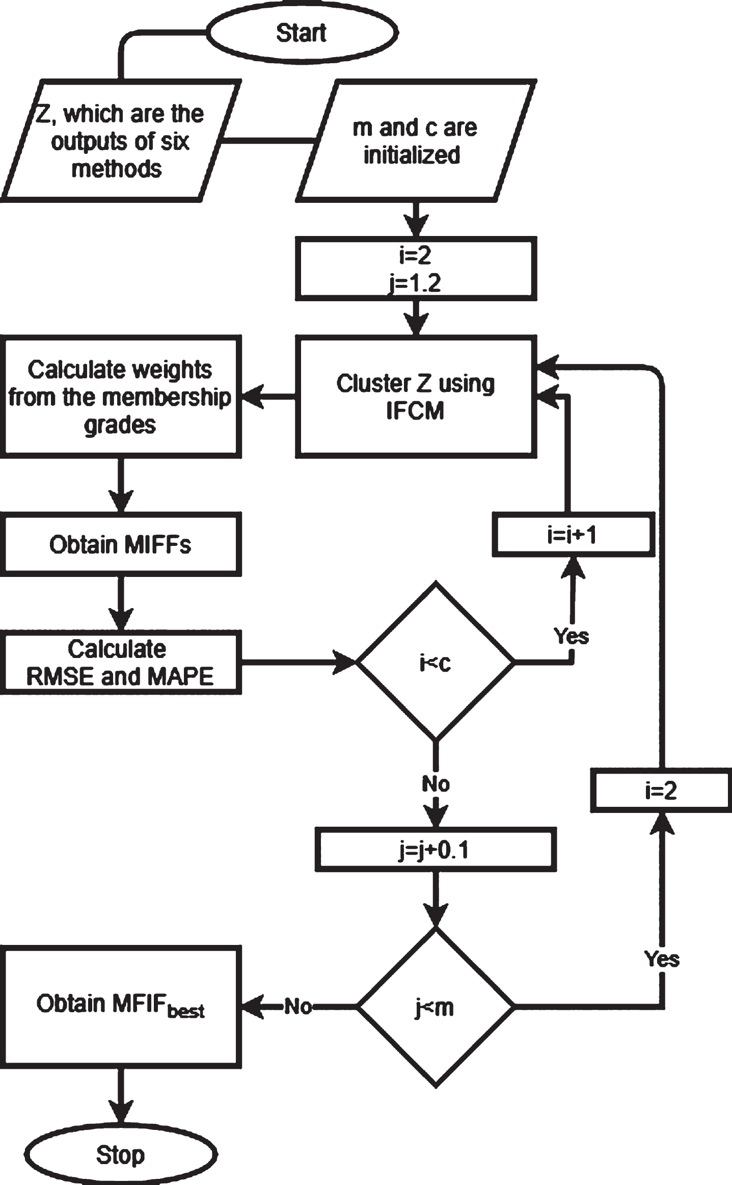
Flowchart of MIFFs.

Step 1. Parameters specification and methods selection.

The lengths of training (ntrain) and test (ntest) datasets for a time series dataset(Y) are determined. The block structure is preferred to discriminate training (Y_train) and test (Y_test) data. Forecasting methods, the number of clusters, alpha - cut and fuzziness index values are determined.

Step 2. Forecasting methods are applied to the training datasets. After training processes, the forecast values are obtained from each method for the test set. Moreover, if the forecast results are obtained from the literature, there is no need for the training processes. The proposed method only needs one step ahead forecasts from all methods for the test dataset.

Step 3. The forecasts of the test dataset from all methods are used as the inputs (X) of MIFFs and divided into two datasets, X_train and X_test. The lengths of X_train (ntrain₁) and X_test (ntest₁) are determined by the user. X_train is used to obtain the degrees of memberships and MIFFs. Then, the function that has the minimum MAPE value is determined as the MIFF_best. X_test is used to compare the performance of the proposed method with the other methods that are obtained from the literature.

Step 4. Z_test, which is standardized inputs of (X_test) is calculated with the formula given in Equation 3, is used to obtain the weights of the methods in a MIFF.

$X = [X_{ij}], i = 1, 2, . ., m; j = 1, 2 . ., {ntrain}_{1}$ (1) $Z = [Z_{ij}], i = 1, 2, . ., m; j = 1, 2 . ., {ntrain}_{1}$ (2) $Z_{. j} = \frac{X_{. j} - mean (X_{. j})}{std . dev (X_{. j})}$ (3) where $X = [\begin{matrix} X_{1, 1} & X_{2, 1} & . & . & X_{m, 1} \\ X_{1, 2} & X_{2, 2} & . & . & X_{m, 2} \\ . & . & . & . & . \\ . & . & . & . & . \\ X_{1, {ntrain}_{1}} & X_{2, {ntrain}_{1}} & . & . & X_{m, {ntrain}_{1}} \end{matrix}]$ where m is the number of methods that are selected for the proposed approach.

Step 5. Z matrix is clustered by using IFCM.

Using IFCM algorithm, the membership degrees for forecasting methods are calculated. In other words, the coefficients of forecasting methods in a function will be determined with the help of IFCM. Using the IFCM algorithm, cluster centers and the degrees of membership (μ (x)) and non-membership (u (x)) are obtained by considering α - cut. If μ (x) < α - cut, then μ (x) =0, and if u (x) < α - cut, then u (x) =0.

Step 5.1. Initialize the number of clusters, the fuzziness index (f), and the centers of the clusters (v_i) randomly.

Step 5.2. Calculate the degrees of membership (μ) and non-membership (u) with the formulas given in Equation (5)–(6):

$\begin{matrix} μ_{ik} = {[\sum_{j = 1}^{c} {(\frac{d (x_{k}, v_{i})}{d (x_{k}, v_{j})})}^{\frac{2}{f - 1}}]}^{- 1}, \\ i = 1, 2, . . c; k = 1, 2, . ., n \end{matrix}$ (4) where d (.) is the Euclidean distance between the kth data in the ith cluster center: $u_{ik} = (1 - μ_{ik}^{α})^{1 / α}, α > 0$ (5) $μ_{ik}^{*} = 1 - u_{ik}$ (6)

Step 5.3. Update the centers of the clusters by using Equation (7): $v_{i} = \frac{\sum_{k = 1}^{n} (μ_{ik}^{*})^{f} x_{k}}{\sum_{k = 1}^{n} (μ_{ik}^{*})^{f}}, i = 1, 2, . . ., c$ (7)

Step 5.4. Stop if the difference between two iterations drops under some threshold; otherwise, go to Step 4.2.

Step 6. Using the degrees of memberships from IFCM, MIFFs are obtained with Equations 8–9.

$\begin{matrix} {MIFF}_{i} (x) = \sum_{j = 1}^{m} w_{ij} x_{j}, i = 1, 2, . ., c; \\ x = (x_{1}, x_{2}, . ., x_{m}) \end{matrix}$ (8) $w_{ij} = \frac{μ_{ij}^{*}}{\sum_{j = 1}^{m} μ_{ij}^{*}}, i = 1, 2, . ., c$ (9) where c represents the number of clusters, MIFF_i is the i^th meta fuzzy forecasting function and x_j is forecast of j^th method and w_ij represents the coefficient of j^th method in the MIFF_i.

Step 7. Forecasts of MIFFs (F_ij ; i = 1, 2, …, c ; j = 1, 2, …, ntrain₁) are obtained for X_{train
_.j} is a vector, consisting of forecasts for j^th data points from m methods. $F_{ij} = {MIFF}_{i} (X_{. j})$ (10) $X_{. j} = {[X_{1 j} X_{2 j} . . . X_{mj}]}^{T}, j = 1, 2, . . ., {ntrain}_{1}$ (11)

Step 8. Determining the MIFF_best. $T = [\begin{matrix} T_{1} \\ T_{2} \\ . \\ T_{{ntrain}_{1}}, \end{matrix}]$ $F = [\begin{matrix} F_{1, 1} & F_{2, 1} & . . & F_{c, 1} \\ F_{1, 2} & F_{2, 2} & . . & F_{c, 2} \\ . . & . . & . . & . . \\ F_{1, {ntrain}_{1}} & F_{2, {ntrain}_{1}} & . . & F_{c, {ntrain}_{1}} \end{matrix}]$ where T is the actual values of X_train and F is the forecasts of MIFFs for X_train.

Using the forecasts and actual values, evaluation criteria (RMSE, MAPE) are calculated. The one that has the minimum evaluation criteria is selected as MIFF_best.

Step 9. The forecasts for the best MIFF are calculated for X_test.

The forecasts for the best MIFF (MIFF_best), ${\hat{F}}_{j}; j = 1, 2, . . ., {ntest}_{1}$ are obtained for X_train. The Input matrix (X) is designed by using obtained forecasts for X_test. X_{test
_.j} is a vector consisting of forecasts for j^th data points from m methods. ${\hat{F}}_{j} = {MIFF}_{best} (X_{{test}_{. j}}), j = 1, 2, . . ., {ntest}_{1}$ (12) $X = [X_{{test}_{ij}}], i = 1, 2, . . ., m; j = 1, 2, . . ., {ntest}_{1}$ (13) $X_{{test}_{. j}} = [X_{{test}_{1 j}} X_{{test}_{2 j}} . . . X_{{test}_{mj}}], j = 1, 2, . . ., {ntest}_{1}$ (14)

Step 10. The evaluation criteria (RMSE, MAPE) is calculated for ${\hat{F}}_{j}$ of the MIFF_best to evaluate the forecasting performances of MIFFs with the methods that are obtained from the literature.

5 Evaluation

The evaluation of MIFFs starts with training by using maximum temperature, monthly average temperature and rainfall datasets of Giresun, Turkey. Then, the forecasts that are obtained from the selected forecasting methods are used as the inputs (X) of MIFFs. Next, X is divided into two sets; X_train and X_test. The length of X_train and X_test are determined by the user. Then, the algorithm is applied to X_train to calculate the weights of the forecasting methods in functions. MIFFs are calculated and the best function is selected as the MIFF_best by using the weights. Further, the methods are evaluated according to RMSE and MAPE values, which are calculated in Equation 15-16 by using X_test. Finally, the performance of MIFFs is validated by using Diebold-Marino and, Tukey post hoc tests.

$RMSE = \sqrt{\frac{1}{n} \sum_{t = 1}^{n} (x_{t} - {\hat{x}}_{t})^{2}}$ (15) $MAPE = \frac{1}{n} \sum_{t = 1}^{n} | \frac{x_{t} - \hat{x_{t}}}{x_{t}} |$ (16)

14 practical time series datasets are used to evaluate the performance of the proposed method. The outcomes of the MIFFs are calculated in R. The first 12 datasets are maximum temperature datasets from Giresun, Turkey whose elements are daily observed from 2006 to 2017 year by year. The observations of the average temperature dataset of Giresun are collected monthly between January 1960 and December 2011. The rainfall dataset is observed monthly from 1960 to 2016 in Giresun, Turkey.

There are two parameters to be adjusted in the proposed method; the fuzziness parameter (m) and cluster numbers (c). Many studies in the literature have been conducted to determine the optimum value of fuzziness parameter by researchers. Pal and Bezdek [38] suggested that [1.5, 2.5] is the optimal value of m. Ozkan and Turksen [22], on the other side, proposed that the upper and lower values of m is varied between 1.4 and 2.6, respectively. Bezdek [23] identified that 2 is the optimum value of m. Because, there is no consensus on determining the optimal value of m, m is searched iteratively between 1.5 to 3 with an increase rate of 0.1 in the study. Optimum cluster numbers are also searched iteratively between 2 and 5. The optimum value of m and c are determined in terms of RMSE/MAPE for the training set.

As an application 6 different selected forecasting benchmarks are aggregated by using MIFFs to obtain more accurate results for temperature and rainfall datasets. Winters additive and multiplicative exponential smoothing methods (Method1 and Method2, respectively), seasonal Holt method (Method3), fuzzy time series network (Method4), time series fuzzy inference system (Method5), and multilayer perceptron artificial neural network (Method6) are trained for all datasets. Multiple inputs, one hidden layer and one output are used as the architecture of ANN and particle swarm optimization method is used to train ANN. The summary of the datasets and the optimum parameter specifications of the datasets for MIFFs are given in Table 1.

Table 1

Summary and parameter determination of the datasets

Datasets	n	ntraining	ntest		m	c
			ntraining₁	ntest₁
Rainfall	360	300	48	12	1.7	3
TempAverage	624	576	36	12	1.9	4
Temp-2006	365	245	90	30	1.7	3
Temp-2007	365	245	90	30	2	3
Temp-2008	366	246	90	30	2	3
Temp-2009	365	245	90	30	1.4	3
Temp-2010	365	245	90	30	1.6	2
Temp-2011	365	245	90	30	1.5	2
Temp-2012	366	246	90	30	1.9	3
Temp-2013	365	245	90	30	1.6	2
Temp-2014	365	245	90	30	1.4	2
Temp-2015	365	245	90	30	2	4
Temp-2016	366	246	90	30	2	4
Temp-2017	365	245	90	30	1.7	3

“ntraining” in the Table 1 is the number of observations in the training dataset that is used to train the selected forecasting methods. By using the trained forecasting methods, rest of the observations are forecasted by using one-step ahead forecast for the given datasets. Then, the forecasts are used as the inputs (X) of MIFFs and divided into two sets by using the block partitioning structure. The first set (X_training) is used to train and calculate the weights of the selected forecasting methods in functions in MIFFs. The forecasts of MIFFs are obtained by using the weights of (X_training) and the second set (X_test). The length of X_training and X_test are represented as ntraining₁ and ntest₁ in Table 1. The optimum values of m and c are searched iteratively for all given datasets and determined as in Table 1.

5.1 Rainfall dataset of Giresun, Turkey

The elements of the rainfall dataset were collected monthly from 1960 to 2016. There are 360 observations in the dataset. In order to train the 6 selected forecasting methods, the last 60 observations are left out of the sample. Thus, the methods are trained by using 300 observations and 60 future points are forecasted by using one-step-ahead forecast approach. Simple average (SimpleA) [26] method, variance covariance method (VCM) [51], artificial neural network (ANN) [10] and meta fuzzy functions (MFFs) [33] based forecast combination methods are used to evaluate the forecasting accuracy of the proposed method for rainfall dataset of Giresun in Table 5.

The forecasts from 6 methods are used as the inputs (X) of MIFFs. The last 12 observations are left out of X. So, the first 48 observations (X_training) are used to calculate the methods’ weights in functions. The weights of the 6 methods and the last 12 observations are used to calculate the forecasts of MIFFs. The weights of the methods for training dataset (X_training) and corresponding RMSE and MAPE values of X_training are given in Table 2. Table 2 is used to determine the MIFF_best by looking at the MAPE values of the functions. MIFFs for rainfall dataset are given in Equation 17-19. MIFF_best that will be used for the future predictions is selected as the second function in terms of MAPE (see Table 3). Table 4 represents that MIFFs obtains more accurate forecasting accuracy by aggregating the selected forecasting benchmarks. Inspecting Table 5, it is clear that the proposed method outperformed some well-known forecast combination techniques in terms of RMSE and MAPE values.

Table 2
Weights of the methods and RMSE values of the functions for the training set

MIFF ₁ MIFF ₂ MIFF ₃

Method1 0.042 0.000 0.300

Method2 0.061 0.000 0.297

Method3 0.370 0.048 0.048

Method4 0.352 0.076 0.093

Method5 0.000 0.812 0.000

Method6 0.175 0.065 0.261

RMSE 0.519 0.282 0.567

MAPE 0.092 0.049 0.099

	MIFF ₁	MIFF ₂	MIFF ₃
Method1	0.042	0.000	0.300
Method2	0.061	0.000	0.297
Method3	0.370	0.048	0.048
Method4	0.352	0.076	0.093
Method5	0.000	0.812	0.000
Method6	0.175	0.065	0.261
RMSE	0.519	0.282	0.567
MAPE	0.092	0.049	0.099

Table 3

Forecasts, RMSE and MAPE values of MIFFs

	Test	MIFF ₁	MIFF ₂	MIFF ₃
49	4.585883	4.368392	4.508602
50	4.55999	4.274074	4.533917
51	4.311693	4.194082	4.372129
52	4.346646	3.170052	4.405857
53	4.344841	4.126871	4.441074
54	4.429526	4.883564	4.502825
55	4.631183	4.167417	4.576967
56	4.557822	4.236087	4.534002
57	4.669473	5.21977	4.570496
58	4.815356	5.21655	4.599993
59	4.762563	4.952812	4.534981
60	4.647198	5.115441	4.555073
RMSE	0.534643	0.203382	0.586136
MAPE	0.105055	0.032967	0.114878

Table 4

The comparison table of MIFF_best and the existing methods and corresponding RMSE and MAPE values for the rainfall dataset

Test	Method1	Method2	Method3	Method4	Method5	Method6	MIFFs
4.275	4.393	4.765	4.746	4.557	4.335	4.290	4.368
4.024	4.507	4.705	4.608	4.604	4.219	4.331	4.274
4.194	4.458	4.620	4.423	4.268	4.188	4.019	4.194
3.506	4.393	4.666	4.389	4.338	2.911	4.152	3.170
4.159	4.387	4.588	4.143	4.497	4.072	4.371	4.127
5.051	4.491	4.533	4.258	4.543	4.982	4.513	4.884
4.168	4.448	4.527	4.287	5.009	4.041	4.681	4.167
4.079	4.365	4.576	4.227	4.903	4.145	4.605	4.236
5.282	4.379	4.541	4.370	5.028	5.329	4.698	5.220
5.701	4.506	4.563	4.780	5.066	5.310	4.551	5.217
4.832	4.438	4.597	5.034	4.715	5.013	4.419	4.953
5.192	4.354	4.687	4.876	4.452	5.232	4.613	5.115
RMSE	0.628	0.659	0.569	0.570	0.227	0.547	0.203
MAPE	0.116	0.135	0.102	0.115	0.036	0.102	0.033

Table 5

The comparison table of MIFF_best and the existing forecast combination methods for the rainfall dataset

Test	SimpleA	MSFE	VCM	ANN	MFFs	MIFFs
4.275	4.514	4.460	4.384	4.134	4.415	4.368
4.024	4.496	4.364	4.491	4.374	4.312	4.274
4.194	4.329	4.163	4.429	4.296	4.237	4.194
3.506	4.141	3.514	4.364	3.196	3.259	3.170
4.159	4.343	4.050	4.372	4.224	4.135	4.127
5.051	4.553	4.610	4.488	5.365	4.849	4.884
4.168	4.499	4.311	4.441	4.545	4.167	4.167
4.079	4.470	4.275	4.359	4.371	4.233	4.236
5.282	4.724	5.004	4.387	5.455	5.169	5.220
5.701	4.796	5.216	4.506	5.495	5.202	5.217
4.832	4.703	5.079	4.446	5.224	4.974	4.953
5.192	4.702	4.991	4.383	5.212	5.107	5.115
RMSE	0.468	0.263	0.617	0.2591	0.208	0.203
MAPE	0.010	0.0467	0.1128	0.0522	0.035	0.033

$\begin{matrix} {MIFF}_{1} = 0.42 * {Method}_{1} + 0.61 * {Method}_{2} + \\ \dots + 0.175 * {Method}_{6} \end{matrix}$ (17) $\begin{matrix} {MIFF}_{best} = {MIFF}_{2} = 0.48 * {Method}_{3} + \\ 0.76 * {Method}_{4} + \dots + 0.065 * {Method}_{6} \end{matrix}$ (18) $\begin{matrix} {MIFF}_{3} = 0.30 * {Method}_{1} + 0.29 * {Method}_{2} + \\ \dots + 0.261 * {Method}_{6} \end{matrix}$ (19)

Diebold-Marino test, which aims to compare the forecasting accuracy of two methods, is used to compare the forecasting performance of MIFFs with other forecasting methods. Table 6 indicates that MIFFs are significantly different SimpleA and VCM although there is no significant difference between MSFE, ANN, MFFs and the MIFFs. However, RMSE and MAPE values of MIFFs, still, indicate a minor improvement on forecasting accuracy.

Table 6

Diebold-Marino test results of the proposed method and other methods for rainfall dataset

Rainfall	SimpleA	MSFE	VCM	ANN	MFFs
DM	–3.725	–1.521	–3.058	–1.035	–0.369
P-value	0.003***	0.157	0.011**	0.323	0.719

DM denotes the test statistics value

*Denotes significance at 10%

**Denotes significance at 5%

***Denotes significance at 1%

5.2 Temperature datasets of Giresun

There are 13 temperature datasets to evaluate the performance of the MIFFs in this section. The first dataset is monthly collected by observing the average temperature of Giresun, Turkey from January, 1960 to December, 2011. The next 12 datasets are daily collected by observing the maximum temperature of Giresun from 2006 to 2017. Each year is evaluated separately. The detailed tables (such as methods’ weights in functions and functions) are given for the first application. The performances of MIFFs of the rest of the datasets are given in comparison tables in terms of RMSE and MAPE values in Tables 12, 13, respectively.

5.2.1 Average temperature

There are 624 observations in average temperature dataset of Giresun, Turkey. The first 624 observations are used to train the selected 6 forecasting methods. The next 48 observations are forecasted by using the selected forecasting methods. The inputs (X) of MIFFs are obtained from the forecasts of 6 different methods. Then, X is divided into two as X_training and X_test. X_training is used to obtain the methods’ weights in functions and to determine the MIFF_best. X_test is used to compare the forecasting performances of the proposed method with the existing ones. The weights of the methods are calculated by the membership degrees of the methods in each cluster and corresponding RMSE and MAPE values are given in Table 7. Table 8 gives the outcomes of 6 selected forecasting methods for X_test and corresponding RMSE and MAPE values.

Table 7
Weights of the methods and RMSE values of the functions for the training set

MIFF ₁ MIFF ₂ MIFF ₃ MIFF ₄

Method1 0.0000 0.0000 0.0000 0.7313

Method2 0.0000 0.0000 0.7388 0.0000

Method3 0.3684 0.0627 0.0000 0.0000

Method4 0.3448 0.1533 0.0779 0.0788

Method5 0.0000 0.5742 0.0000 0.0000

Method6 0.2868 0.2099 0.1833 0.1899

RMSE 1.8470 1.4866 2.6861 2.7719

MAPE 0.1341 0.0963 0.1824 0.1821

	MIFF ₁	MIFF ₂	MIFF ₃	MIFF ₄
Method1	0.0000	0.0000	0.0000	0.7313
Method2	0.0000	0.0000	0.7388	0.0000
Method3	0.3684	0.0627	0.0000	0.0000
Method4	0.3448	0.1533	0.0779	0.0788
Method5	0.0000	0.5742	0.0000	0.0000
Method6	0.2868	0.2099	0.1833	0.1899
RMSE	1.8470	1.4866	2.6861	2.7719
MAPE	0.1341	0.0963	0.1824	0.1821

Table 8

Forecasts, RMSE and MAPE values of MIFFs

Obs.	MIFF ₁	MIFF ₂	MIFF ₃	MIFF ₄
37	8.760	7.627	10.568	11.194
38	7.917	7.152	4.671	4.972
39	8.940	7.535	5.625	4.802
40	11.401	10.631	9.042	9.018
41	15.287	14.312	11.361	11.850
42	20.826	21.691	20.173	20.337
43	23.838	23.590	25.325	24.909
44	24.275	23.884	27.585	27.440
45	21.928	22.585	22.641	23.633
46	18.022	15.648	19.635	19.298
47	13.015	12.214	10.668	10.146
48	9.672	9.208	3.792	3.493
RMSE	1.689	1.297	3.096	3.163
MAPE	0.115	0.085	0.225	0.231

It is clear from Table 7 that the best performances are obtained from the second function in terms of both RMSE and MAPE values. Therefore, the future forecasts are calculated by using the second function that is given in Equation 20. Four methods contribute the performance of the second function. Although the most contribution is carried out from the fifth method, the third, fourth and sixth methods also have some effect on the forecasting performances of MIFF₂.

Table 8 represents the forecasting performances of the all functions and corresponding RMSE and MAPE values. Simple average (SimpleA) method, variance covariance method (VCM), artificial neural network (ANN) and meta fuzzy functions (MFFs) based forecast combination methods are used to evaluate the forecasting accuracy of the proposed method for average temperature of Giresun in Table 10. Results in Tables 9 and 10 show that MIFF_best outperformed the other functions and the selected forecasting methods in terms of RMSE and MAPE values. $\begin{matrix} {MIFF}_{1} = 0.3684 * Method 3 + 0.3448 * Method 4 \\ + 0.2868 * Method 6 \end{matrix}$ (20) $\begin{matrix} {MIFF}_{best} = {MIFF}_{2} = 0.0627 * Method 3 + 0.1533 * \\ Method 4 + 0.5742 * Method 5 + 0.2099 * Method 6 \end{matrix}$ (21) $\begin{matrix} {MIFF}_{3} = 0.7388 * Method 2 + 0.0779 * Method 4 \\ + 0.1833 * Method 6 \end{matrix}$ (22) $\begin{matrix} {MIFF}_{4} = 0.7313 * Method 1 + 0.0788 * Method 4 \\ + 0.1899 * Method 6 \end{matrix}$ (23)

Table 9

The comparison table of MIFF_best and the existing methods and corresponding RMSE and MAPE values

Test Data	Method1	Method2	Method3	Method4	Method5	Method6	MIFFs
8	11.7063	10.8425	7.6739	8.6615	6.3783	10.2735	7.627
6.9	3.8901	3.5235	7.7796	8.1412	6.5734	7.8243	7.152
8.1	3.5573	4.7133	8.8395	10.4544	6.7182	7.2505	7.535
9.6	8.5394	8.5824	11.3858	13.3696	10.3934	9.0560	10.631
15.1	11.0988	10.4581	15.8021	16.9509	14.0622	12.6249	14.312
20.7	20.4633	20.2307	20.7933	22.3762	22.5884	19.0033	21.691
24.5	25.5128	26.0482	23.6804	25.1234	23.5722	22.4942	23.590
23.6	28.7663	28.9089	24.3235	24.9948	23.7353	23.3481	23.884
21.2	24.3519	22.9754	20.7027	24.3776	23.0542	20.5564	22.585
15.3	19.9507	20.3738	16.9270	20.7093	13.9556	16.2000	15.648
8.6	9.5020	10.2247	13.0922	14.8919	11.9722	10.6587	12.214
10.2	1.6845	2.1509	10.1264	11.1857	9.2885	7.2674	9.208
RMSE	4.0128	3.8801	1.5650	3.0307	1.5342	1.6881	1.297
MAPE	0.2917	0.2817	0.1017	0.2138	0.1136	0.1278	0.085

Table 10

The comparison table of MIFF_best and the existing forecast combination methods

Test Data	SimpleA	MSFE	VCM	ANN	MFF	MIFF
8	9.2560	10.53	5.77	6.31	7.3025	7.627
6.9	6.2887	4.15	8.98	5.22	6.9839	7.152
8.1	6.9222	4.99	8.91	6.21	7.3109	7.535
9.6	10.2211	9.42	10.29	10.51	10.5883	10.631
15.1	13.4995	11.91	15.96	14.43	14.2295	14.312
20.7	20.9092	20.90	19.49	22.22	21.9951	21.691
24.5	24.4052	25.88	21.41	24.06	23.6138	23.590
23.6	25.6795	28.55	21.67	24.64	23.8459	23.884
21.2	22.6697	23.82	16.65	22.76	22.8413	22.585
15.3	18.0194	20.20	12.05	16.26	15.2290	15.648
8.6	11.7236	10.75	12.32	12.36	12.1632	12.214
10.2	6.9506	3.36	11.90	8.07	9.2287	9.208
RMSE	1.8379	3.4465	2.4811	1.7342	1.3451	1.297
MAPE	0.1327	0.2474	0.1751	0.1454	0.0882	0.085

By comparing the forecasting results of the existing combination methods with MIFFs, MIFFs outperformed MSFE, VCM and ANN. In addition, DM tests (see Table 11) suggest that there is no significant difference between SimpleA, ANN and MIFFs.

Table 11

Diebold-Marino test results for forecasted IEX using the proposed method and other methods

	SimpleA	MSFE	VCM	ANN	MFFs
DM	–1.60	–2.39	–2.72	–3.23	–1.29
P-value	0.14	0.035**	0.020**	0.008***	0.222

DM denotes the test statistics value.

*Denotes significance at 10%.

**Denotes significance at 5%.

***Denotes significance at 1%.

5.2.2 Maximum temperature datasets

12 real-time series datasets are evaluated by using the outcomes of six different forecasting methods as the inputs of MIFFs in this section. The summary of the datasets, length of training and test datasets, the optimum value of m and optimum cluster numbers are given in Table 1. The search space for the optimum value of m and the cluster numbers are varied between 1.5 to 2.5 with an increment of 0.1 and between 2 to 5, respectively. The results of MIFF_best and the selected forecasting methods in terms of RMSE and MAPE values are given in Tables 12 and 13, respectively.

Table 12
RMSE values of the selected methods and MIFFs for Rainfall datasets of Giresun

Years Method1 Method2 Method3 Method4 Method5 Method6 SimpleA MFFs MIFFs

2006 2.875 3.213 2.828 2.841 1.249 2.654 2.610 1.249 1.249

2007 1.970 2.619 2.087 1.859 1.629 2.132 2.049 1.325 1.299

2008 2.789 3.975 2.769 2.543 2.052 2.992 2.853 1.789 1.609

2009 3.859 3.680 3.284 3.086 1.030 3.825 3.127 1.030 1.030

2010 4.436 5.040 4.091 4.101 1.116 4.185 3.828 0.986 0.931

2011 3.284 3.747 3.078 3.175 0.741 3.268 2.882 0.741 0.741

2012 2.963 3.341 2.656 2.809 0.826 3.052 2.608 0.799 0.766

2013 2.898 3.875 3.712 2.914 1.775 3.718 3.149 1.623 1.627

2014 3.550 3.993 3.251 3.302 1.028 3.242 3.061 1.036 1.028

2015 2.568 3.394 2.603 2.626 1.145 2.458 2.466 1.085 1.061

2016 3.222 3.246 3.019 3.042 1.103 2.943 2.763 1.060 1.051

2017 3.069 3.549 2.868 2.938 0.854 3.030 2.718 0.851 0.776

Mean 3.124 3.639 3.020 2.936 1.212 3.125 2.843 1.131 1.097

Years	Method1	Method2	Method3	Method4	Method5	Method6	SimpleA	MFFs	MIFFs
2006	2.875	3.213	2.828	2.841	1.249	2.654	2.610	1.249	1.249
2007	1.970	2.619	2.087	1.859	1.629	2.132	2.049	1.325	1.299
2008	2.789	3.975	2.769	2.543	2.052	2.992	2.853	1.789	1.609
2009	3.859	3.680	3.284	3.086	1.030	3.825	3.127	1.030	1.030
2010	4.436	5.040	4.091	4.101	1.116	4.185	3.828	0.986	0.931
2011	3.284	3.747	3.078	3.175	0.741	3.268	2.882	0.741	0.741
2012	2.963	3.341	2.656	2.809	0.826	3.052	2.608	0.799	0.766
2013	2.898	3.875	3.712	2.914	1.775	3.718	3.149	1.623	1.627
2014	3.550	3.993	3.251	3.302	1.028	3.242	3.061	1.036	1.028
2015	2.568	3.394	2.603	2.626	1.145	2.458	2.466	1.085	1.061
2016	3.222	3.246	3.019	3.042	1.103	2.943	2.763	1.060	1.051
2017	3.069	3.549	2.868	2.938	0.854	3.030	2.718	0.851	0.776
Mean	3.124	3.639	3.020	2.936	1.212	3.125	2.843	1.131	1.097

Table 13

MAPE values of the selected methods and MIFFs for Rainfall datasets of Giresun

Years	Method1	Method2	Method3	Method4	Method5	Method6	SimpleA	MFFs	MIFFs
2006	0.981	1.083	1.030	1.071	0.479	0.964	0.935	0.479	0.479
2007	0.149	0.245	0.181	0.149	0.150	0.188	0.177	0.124	0.121
2008	0.211	0.414	0.240	0.186	0.158	0.276	0.247	0.119	0.100
2009	0.196	0.201	0.160	0.160	0.056	0.188	0.160	0.056	0.056
2010	0.240	0.290	0.218	0.223	0.053	0.213	0.206	0.057	0.049
2011	0.192	0.245	0.180	0.185	0.048	0.188	0.173	0.048	0.048
2012	0.180	0.231	0.146	0.167	0.060	0.186	0.162	0.051	0.048
2013	0.329	0.496	0.476	0.321	0.226	0.478	0.388	0.222	0.221
2014	0.192	0.221	0.178	0.176	0.048	0.174	0.165	0.046	0.048
2015	0.228	0.298	0.228	0.228	0.110	0.212	0.217	0.105	0.102
2016	0.293	0.306	0.290	0.291	0.111	0.311	0.267	0.108	0.108
2017	0.171	0.224	0.166	0.169	0.052	0.171	0.159	0.052	0.047
Mean	0.280	0.354	0.291	0.277	0.129	0.296	0.271	0.122	0.119

The outcomes of MIFFs outperform the other methods in both tables by looking at the average of RMSE and MAPE values. Most of the time MIFFs approach improves the forecasting performances by aggregating different forecasting methods in functions. However, if the aggregation of the forecasting methods does not improve the forecasting performances, then, the proposed approach is able to determine the method that performs best in terms of MAPE values for a given dataset. Because Method 5 dominates the other five methods most of the time for temperature datasets of Giresun, Turkey, MIFF_best contains Method 5 with higher effect size for almost all years.

The one way analysis of variance (ANOVA) test is applied to see the significant difference among the means of RMSE values for all methods. The obtained ANOVA table is given in Table 14. According to statistical analysis, there is a significant difference among the methods. To determine homogenous sub-groups, Tukey post hoc test is applied and the results are given in Table 15. According to Table 15, the proposed method is grouped with the Method5 (TS-FIS) and MFFs approach. Other methods can create different two sub-groups without contain the proposed MIFFs method.

Table 14

The one way ANOVA results to compare performance of all methods for temperature datasets

Source	Type III Sum of Squares	df	Mean Square	F	Sig.
Corrected Model	97,683a	8	12210	50467	0.000
Intercept	652884	1	652884	2698466	0.000
Group	97683	8	12210	50467	0.000
Error	23953	99	0.242
Total	774519	108
Corrected Total	121635	107	a. R Squared = 0.803 (Adjusted R Squared = 0.787).

Table 15

The homogenous sub-grups according to post hoc test

Group	N	Subsets
		1	2	3
MIFFs	12	10973
MFFs	12	11312
Method5	12	12123
SimpleA	12		28428
Method4	12		29363
Method3	12		30205	30205
Method1	12		31236	31236
Method6	12		31249	31249
Method2	12			36393
Sig.		1000	0.893	0.064

Means for groups in homogeneous subsets are displayed.

Based on observed means.

The error term is Mean Square(Error) = 0.242.

a. Uses Harmonic Mean Sample Size = 12.

b. Alpha = 0.05.

6 Conclusions

A novel approach based on IFCM and MFFs is introduced to aggregate 6 selected forecasting methods in the study. The aim of the study is to combine the selected forecasting methods into functions by looking at their performances for a given time series dataset. In other words, collecting the methods, which perform better for a given dataset in terms of some evaluation criteria, in a cluster with higher degree of membership values is the focus of the paper. Some remarks of MIFFs are listed below.

6 different forecasting methods that were proposed under different circumstances are selected for the proposed method. Three of the selected forecasting methods are called as the classical time series approaches while the rest are called as non-classical time series forecasting methods. ANN, FISs, and FTS approaches are most used techniques as an alternative (non-classical) forecasting method in the literature. Thus, a method under each of these techniques is selected for the proposed method.

IFCM is employed to improve the performance of the proposed by quantifying the hesitancy of an object in a cluster.

The scope of the MIFFs is the aggregate the information of selected forecasting methods in functions by considering their forecasting performances for a given dataset. Therefore, MIFFs is an adaptive method that adjusts itself for a given dataset. For example, while method A can dominate the other methods for a dataset, method B can dominate method A for different datasets. Thus, while method A will be selected in the best function with higher weight, method B will be selected in the best function for different datasets.

Although MIFFs are usually able to increase the forecasting accuracy of 6 different forecasting methods by aggregating them in functions, they, at least, guarantees to pick the best forecasting method in terms of MAPE/RMSE among 6 methods.

In the paper, we propose a naive way to combine different forecasting methods in functions to get more reliable forecasting results in terms of some evaluation criteria. We use 14 different meteorological datasets from Giresun, Turkey. From the results, we are able to claim that MIFFs have the ability to improve the forecasting accuracy by aggregating different forecasting methods. For some datasets, MIFFs produced the outcomes of the best forecasting method. For example, the performances of MFFs and MIFFs are almost identical for Tables 5 and 10 because TS-FIS has outstanding forecasting performance compared to other forecasting methods. Thus, TS-FIS stands alone in a cluster for both MFFs and MIFFs. Although, there is no significant difference between MFFs and MIFFs, there is still improvement on forecasting performance for the proposed method. However, MIFF, usually, produced better outcomes than the best method by aggregating more than one method in functions. It is possible to increase the number of forecasting methods in the proposed method. We believe that the more forecasting methods in the MIFFs will give the better forecasting accuracy.

Declaration of competing interest

The authors declare that they have no known competing financial interests or personal relationships that could have appeared to influence the work reported in this paper.

References

Khosravi

, Koury

R.N.N.

, Machado

and Pabon

J.J.G.

, Prediction of wind speed and wind direction using artificial neural network, support vector regression and adaptive neuro-fuzzy inference system, Sustainable Energy Technologies and Assessments 25 (2018), 146–160.

Safari

and Davallou

, Oil price forecasting using a hybrid model, Information Sciences 148 (2018), 49–58.

Shamseldin

A.Y.

, O’Connor

K.M.

and Nasr

A.E.

, A comparative study of three neural network forecast combination methods for simulated river flows of different rainfall–runoff models, Hydrological Sciences Journal 52(2) (2007), 896–916.

Chang

, Resolving the forecasting problems of overshoot and volatility clustering using ANFIS coupling nonlinear heteroscedasticity with quantum tuning, Fuzzy Sets and Systems 159(23) (2008), 3183–3200.

Sarica

, Egrioglu

and Asikgil

, A new hybrid method for time series forecasting: AR-ANFIS, Neural Computing and Applications 29(3) (2018), 749–760.

Kocak

, Egrioglu

and Bas

, A new deep intuitionistic fuzzy time series forecasting method based on long shortterm memory, The Journal of Supercomputing (2020), 1–9.

Lemke

and Gabrys

, Meta-learning for time series forecasting and forecast combination, Neurocomputing 73(10-12) (2010), 2006–2016.

Luo

, Tan

, Wang

and Zheng

, An evolving recurrent interval type-2 intuitionistic fuzzy neural network for online learning and time series prediction, Applied Soft Computing 78 (2019), 150–163.

Holt

C.C.

, Forecasting seasonals and trends by exponentially weighted moving averages, Pittsburgh, Pa.: Carnegie Institute of Technology, Graduate school of Industrial Administration, 1957.

10.

Aladag

C.H.

, Egrioglu

and Yolcu

, Forecast Combination by Using Artificial Neural Networks, Neural Processing Letters 32(3) (2010), 269–276.

11.

Granger

C.W.J.

and Ramanathan

, Improved methods of combined forecasts, Journal of Forecasting 3(2) (1984), 1178–1188.

12.

Chen

and Zhang

, Time series prediction based on ensemble ANFIS, Proceedings of the fourth international conference on machine learning and cybermetics (2005), 3353–3356.

13.

Rumelhart

D.E.

, Hinton

G.E.

and Williams

R.J.

, Learning internal representations by error propagation, California Univ San Diego La Jolla Inst for Cognitive Science (1985).

14.

Bas

, Egrioglu

, Aladag

C.H.

and Yolcu

, Fuzzy-Time-Series Network used to forecast linear and nonlinear time series, Applied Intelligence 43(2) (2015), 343–355.

15.

Egrioglu

, Aladag

C.H.

, Yolcu

and Bas

, Recurrent multiplicative neuron model artificial neural network for non-linear time series forecasting, Neural Processing Letters 41(2) (2015), 249–258.

16.

Egrioglu

, Aladag

C.H.

, Yolcu

, Basaran

M.A.

and Uslu

V.R.

, A new hybrid approach based on SARIMA and partial high order bivariate fuzzy time series forecasting model, Expert Systems with Applications 36(5) (2009), 7424–7434.

17.

Mamdani

E.H.

and Assilian

, An experiment in linguistic synthesis with a fuzzy logic controller, International Journal of Man-Machine Studies 7(1) (1975), 1–13.

18.

Elliott

and Timmermann

, Optimal forecast combination under regime switching, International Economic Review 46(4) (2005), 1081–1102.

19.

Box

G.E.P

and Jenkins

G.M

, Time Series Analysis: Forecasting and Control, Holdan-Day, San Francisco,CA, 1976.

20.

Zhang

G.P

, Time series forecasting using a hybrid ARIMA and neural network model, Neurocomputing 50 (2003), 159–175.

21.

Turksen

I.B.

, Fuzzy functions with LSE, Applied Soft Computing 8(3) (2008), 1178–1188.

22.

Ozkan

and Turksen

I.B.

, Upper and lower values for the level of fuzziness in FCM, Information Sciences 177(23) (2007), 5143–5152.

23.

Bezdek

J.C.

, A physical interpretation of fuzzy ISODATA, Readings in Fuzzy Sets for Intelligent Systems (1993), 615–616.

24.

Bezdek

J. C.

, Ehrlich

and Full

, FCM: The fuzzy c-means clustering algorithm, Computers and Geosciences 10(2-3) (1984), 191–203.

25.

Jang

J.S.R.

, ANFIS: adaptive-network-based fuzzy inference system, IEEE Transactions on Systems, Man, and Cybernetics 23(3) (1993), 665–685.

26.

Bates

J.M.

and Granger

C.W.J.

, The combination of forecast, Journal of the Operational Research Society 20(4) (1969), 451–468.

27.

Bisht

and Kumar

, Hesitant fuzzy set based computational method for financial time series forecasting, Granular Computing 4(4) (2019), 655–669.

28.

Gupta

K.K.

and Kumar

, Hesitant probabilistic fuzzy set based time series forecasting method, Granular Computing 4(4) (2019), 739–758.

29.

Atanassov

K.T.

, Intuitionistic fuzzy sets, In Intuitionistic Fuzzy Sets, (pp. 1–137). Physica, Heidelberg, 1999.

30.

Wang

, Wang

, Qu

and Liu

, Optimal forecast combination based on neural networks for time series forecasting, Applied Soft Computing 66 (2018), 1–17.

31.

Zadeh

L.A.

, Outline of a new approach to the analysis of complex systems and decision process, IEEE Transactions on Systems, Man, and Cybernetics 3(1) (1973), 28–44.

32.

Chen

M.Y.

and Chen

B.T.

, A hybrid fuzzy time series model based on granular computing for stock price forecasting, Information Sciences 294 (2015), 227–241.

33.

Tak

, Meta fuzzy functions: Application of recurrent type-1 fuzzy functions, Applied Soft Computing 73 (2018), 1–13.

34.

Tak

, Type-1 recurrent intuitionistic fuzzy functions for forecasting, Expert Systems with Applications 140 (2020), Article ID:112913.

35.

Tak

, Meta fuzzy index functions, Communications Faculty of Sciences University of Ankara Series A1 Mathematics and Statistics 69(1) (2020), 654–667.

36.

Tak

and Gok

, Dating currency crises and designing early warning systems: Meta-possibilistic fuzzy index functions, International Journal of Finance and Economics, (2020), 1–18.

37.

Tak

, Evren

A.A.

, Tez

and Egrioglu

, Recurrent type-1 fuzzy functions approach for time series forecasting, Applied Intelligence 48(1) (2018), 68–77.

38.

Pal

N.R.

and Bezdek

J.C.

, On cluster validity for the fuzzy c-means model, IEEE Transactions on Fuzzy systems 3(3) (1995), 370–379.

39.

Cagcag

, Yolcu

, Egrioglu

and Aladag

C.H.

, A Novel Seasonal Fuzzy Time Series Method To The Forecasting Of Air Pollution Data In Ankara, American Journal Of Intelligent Systems 3(1) (2013), 13–19.

40.

Gundogdu

, Egrioglu

, Aladag

C.H.

and Yolcu

, Multiplicative neuron model artificial neural network based on gauss activation function, Neural Computing and Applications 27(4) (2015), 927–935.

41.

Hajek

, Froelich

and Prochazka

, Intuitionistic Fuzzy Grey Cognitive Maps for Forecasting Interval-Valued Time Series, Neurocomputing (2020).

42.

Newbold

and Granger

C.W.J.

, Experience with forecasting time series and combination of forecasts, Journal of the Royal Statistical Society, Series A 137(2) (1974), 131–165.

43.

Jiang

, Yang

, Li

and Li

, Inbound tourism demand forecasting framework based on fuzzy time series and advanced optimization algorithm, Applied Soft Computing 92 (2000), 106320.

44.

and Chan

M.F.

, Predictive time-series modeling using artificial neural networks for Linac beam symmetry: an empirical study, Annals of the New York Academy of Sciences 1387(1) (2017), 84–94.

45.

Song

and Chissom

B.S.

, Fuzzy time series and its models, Fuzzy Sets and Systems 54(3) (1993), 269–277.

46.

Schalkoff

, Pattern Recognition: Statistical. Structural and Neural Approaches, Wiley, New York, 1992.

47.

Beyhan

and Alci

, Fuzzy functions based arx model and new fuzzy basis function models for nonlinear system identification, Applied Soft Computing 10(2) (2010), 439–444.

48.

Hassan

S.G.

, Iqbal

, Garg

, Hassan

, Shuangyin

and Kieuvan

T.T.

, Designing Intuitionistic Fuzzy Forecasting Model Combined With Information Granules and Weighted Association Reasoning, IEEE Access 8 (2020), 141090–141103.

49.

Chen

S.M.

and Phuong

B.D.H.

, Fuzzy time series forecasting based on optimal partitions of intervals and optimal weighting vectors, Knowledge-Based Systems 118 (2017), 204–216.

50.

Makridakis

and Winkler

R.L.

, Averages of forecasts: Some empirical results, Management Science 29(9) (1983), 987–996.

51.

Gupta

and Wilton

P.C.

, Combination of forecasts: an extension, Management Science 33(3) (1987), 356–372.

52.

Xian

, Zhang

, Xiao

and Pang

, A novel fuzzy time series forecasting method based on the improved artificial fish swarm optimization algorithm, Soft Computing 22(12) (2018), 3907–3917.

53.

Takagi

and Sugeno

, Fuzzy identification of systems and its applications to modeling and control, IEEE Transactions on Systems, Man, and Cybernetics 15(1) (1985), 116–132.

54.

Yolcu

, Egrioglu

and Aladag

C.H.

, A new linear and nonlinear artificial neural network model for time series forecasting, Decision Support Systems 54 (2013), 1340–1347.

55.

Yolcu

, Egrioglu

and Bas

, A novel Holt’s method with seasonal component based on particle swarm optimization, 10th International Statistics Congress, Abstract book (2017), 86.

56.

Yolcu

, Bas

and Egrioglu

, A new fuzzy inference system for time series forecasting and obtaining the probabilistic forecasts via subsampling block bootstrap, Journal of Intelligent and Fuzzy Systems 35(2) (2018), 2349–2358.

57.

Khatibi

and Montazer

G.A.

, Intuitionistic fuzzy set vs. fuzzy set application in medical pattern recognition, Artificial Intelligence in Medicine 47(1) (2009), 43–52.

58.

McCulloch

W.S.

and Pitts

, A logical calculus of the ideas immanent in nervous activity, The bulletin of mathematical biophysics 5(4) (1943), 115–133.

59.

Fan

, Wang

and Zhang

, Network traffic forecasting model based on long-term intuitionistic fuzzy time series, Information Sciences 506 (2020), 131–147.