A hybrid algorithm for electric vehicle routing problem with nonlinear charging

2.1 Problem definition

In this section, the characteristics of the EVRPTW-NL can be generalized as follows:

There are some homogeneous EVs.

In a realistic logistic system, a nonlinear function is related to the charging time. The EVs that start from the depot are assumed to be fully battery capacity, and all the charging stations can handle an unlimited number of vehicles simultaneously. It might be profitable to charge overnight at the depot from a practical point of view [48]. Meanwhile, under fierce market competition, attention must be paid to customer satisfaction. If vehicles arrive within the time windows of the customer, it will achieve a higher satisfaction level.

Moreover, the calculation of the customer satisfaction level is divided into two categories. One is based on the number of customers, which depends on the proportion of the number of customers (i.e., providing service in advance or delay) to the total customers. The other task is to use the time window to calculate the customer satisfaction level. If the time window is a hard window, the value of customer satisfaction is 0 or 1. A triangular fuzzy membership function describes the satisfaction level under the fuzzy time windows. Adopting a rating level method is different from other literature [29, 30]. The superiority of this method are as follows: First, the more important the customer, the stricter the time window; Second, a proportion is calculated by the time interval, which represented by the customer satisfaction level, and the level is integrated into the objective. These superiority make this problem more realistic.

It has following assumptions in this paper:

Each customer must be served by only one vehicle.

2.2 Problem formulation

The EVRPTW-NL is defined on the graph G = (V, A), where V = {0} ∪ I ∪ F′. The 0 represents the depot, I and F′ are the set of customers and dummy vertices of charging stations, respectively. Let A = {(i, j) |i, j ∈ V, i ≠ j} be the set of arcs connecting vertices of V. Each arc (i, j) ∈ A is associated with a trip time t _ij and a battery consumption e _ij . In this paper, the battery consumption is equal to the distance. Each customer i ∈ I has a service time s _i . In canonical VRPTW, every customer i ∈ I equips a time window [a _i , b _i ]. In this study, it sets a preferred time window [E_ti, L_ti] and an allowable time window [EE_ti, LL_ti]. Customers cannot visit after their allowable time window [49]. Each charging station corresponds to a piecewise linear approximation of the charging function which modified from Montoya et al. [11]. The piecewise linear approximation of the charging function according to the different charging level which corresponding to the different speeds of charging. There are four level stages in this function which corresponding different charging speed for each stage. The problem is to minimize the total trip time and maximize the customer satisfaction value.

The parameters and decision variables are defined as follows:

In addition, the corresponding formulas are shown as follows:

Objective: min w ( ∑ i , j ∈ V V t ij x ij + ∑ i ∈ F ′ F ′ Δ i ) - ( 1 - w ) ∑ i = 1 I sv i(1)

Subject to:

∑ j ∈ V , i ≠ j x ij = 1 ∀ i ∈ I ( 2 ) ∑ j ∈ V , i ≠ j x ji - ∑ j ∈ V , i ≠ j x ij = 0 ∀ i ∈ I ( 3 ) { a 0 = B 0 ⩽ a i ⩽ B ∀ i ∈ V ( 4 ) e ij x ij - B ( 1 - x ij ) ⩽ a i - a j ∀ i ∈ V , j ∈ I ( 5 ) e ij x ij + B ( 1 - x ij ) ⩾ a i - a j ∀ i ∈ V , j ∈ I ( 6 ) e ij x ij - B ( 1 - x ij ) ⩽ a i - q j s ∀ i ∈ V , j ∈ F ′ ( 7 ) e ij x ij + B ( 1 - x ij ) ⩾ a i - q j s ∀ i ∈ V , j ∈ F ′ ( 8 ) a i ⩾ e i 0 x i 0 ∀ i ∈ V ( 9 ) a i = q i d ∀ i ∈ F ′ ( 10 ) 0 ⩽ q i s ⩽ q i d ⩽ B ∀ i ∈ F ′ ( 11 ) s l + ( z il - 1 ) ⩽ q i s B ⩽ s l + 1 + ( 1 - z il ) ∀ i ∈ F ′ , l ∈ R ( 12 ) ∑ l ∈ R z il = 1 ∀ i ∈ F ′ ( 13 ) q i s B ⩾ k l t ′ + b l - M ( 1 - z il ) ∀ i ∈ F ′ , l ∈ R ( 14 ) q i s B ⩽ k l t ′ + b l + M ( 1 - z il ) ∀ i ∈ F ′ , l ∈ R ( 15 ) s l + ( d il - 1 ) ⩽ q i d B ⩽ s l + 1 + ( 1 - d il ) ∀ i ∈ F ′ , l ∈ R ( 16 ) ∑ l ∈ R d il = 1 ∀ i ∈ F ′ ( 17 ) q i d B ⩾ k l t ″ + b l - M ( 1 - d il ) ∀ i ∈ F ′ , l ∈ R ( 18 ) q i d B ⩽ k l t ″ + b l + M ( 1 - d il ) ∀ i ∈ F ′ , l ∈ R ( 19 ) Δ i = t ″ - t ′ ∀ i ∈ F ′ ( 20 ) EE ti ⩽ t i ⩽ LL ti ∀ i ∈ I ( 21 ) st i + s i + t ij x ij - M ( 1 - x ij ) ⩽ t j ∀ i , j ∈ I ( 22 ) ∑ i ∈ F ′ Δ i + ∑ i ∈ V ∑ j ∈ V t ij x ij + ∑ i ∈ I s i ⩽ T max ( 23 ) ∑ i ∈ I ∑ j ∈ I d i x ij ⩽ Q ( 24 ) t ′ ⩾ 0 , t ″ ⩾ 0 , Δ i ⩾ 0 ∀ i ∈ F ′ ∀ i ∈ F ′ ( 25 ) sv i = { 1 , 1 - E ti - t i E ti - EE ti , 1 - t i - L ti LL ti - L ti E ti ⩽ t i ⩽ L ti EE ti ⩽ t i ⩽ E ti L ti ⩽ t i ⩽ LL ti ( 26 )

Different weights have different optimization effects on each objective of the multi-objective problems, and the weight sum method can well balance of the optimization between two objectives. In this paper, the weighted sum method is used to solve the problem, which gives the corresponding weight value according to the importance of each objective, and then converts the problem into single objective by optimizing its linear combination [50–52]. The objective function of Equation (1) is to minimize the weighted sum of the total trip time and customer satisfaction value, i.e., minimize the total trip time and maximize the customer satisfaction value. Equation (2) ensures that each customer is served only once. Equation (3) indicates that the number of arrivals and leaves the same vertex is equal. Equation (4) ensures the EV is fully charged departs from the depot, and the remaining battery capacity of the EV maintains between 0 and the maximum battery capacity. Equations (5)–(8) track of battery consumption at each vertex. Equations (5)-(6) calculate the battery consumption between two adjacent customers. Equations (7)-(8) compute the battery consumption between the customer and the charging station. Equation (9) guarantees the EV with the remaining battery level can reach the depot. Equation (10) resets the battery capacity of the EV after charging and the remaining battery capacity of the EV is equal to the battery level after charging. Equation (11) tracks of battery capacity at each charging station and the remaining battery capacity of the EV maintains between 0 and the maximum battery capacity. Equations (12)–(19) define the remaining battery capacity when the EV arrives at (or leaves) the charging station and the charging time. Equations (12)–(15) calculate the charging time corresponding to the remaining battery capacity of the EV when it arrives at the charging station. Equations (12)-(13) denote the interval in which the remaining battery capacity (in percentage) when the EV arrives at the charging station belongs to the nonlinear charging function. Equations (14)-(15) calculate the current time corresponding to the current battery capacity. Equations (16)–(19) calculate the current time corresponding to the battery level after charging for the EV and the approach is the same as above. Equation (20) is the time difference between t′ and t″. Equation (21) is the time window constraints. Equation (22) represents the time relationship between two adjacent customers. Equations (23)-(24) guarantee that the sum of the total trip time and the demand of customers do not exceed the maximum trip time and load capacity of the EV, respectively. Equation (25) states the range of the variable. Equation (26) calculates the customer satisfaction level that discussed in sub-section 4.4 in detail.

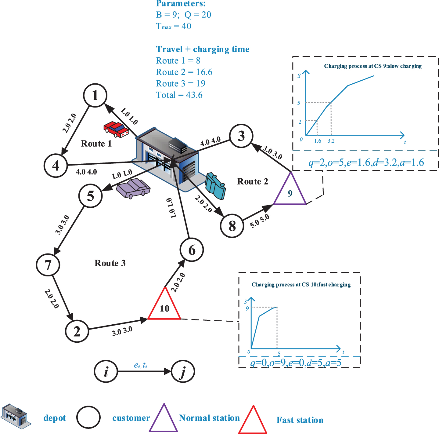
As depicted in Fig. 1, there are eight customers and two charging stations. Customer parameters are shown in Table 1. The tolerate time is 0.5 units and the service duration for each customer is 0.5 units. The charging stations contain two types (normal and fast) of charging stations. The piecewise linear function maps the battery capacity q and o to the charging time e to d so as to estimate the time spent at the charging station, and a presents the time difference between e and d. The information of the EV is depicted in Fig. 1 (the maximum load capacity is 20, the maximum battery capacity is 9 units, and the maximum trip time is 40 units). In this example, Route 1 does not require visiting any charging stations. Route 2 recharges at the No.9 charging station, where the EV arrives at the charging station with the zero remaining battery capacity and recharges to o = 5. It used the piecewise linear function to estimate the recharging time. Therefore, Route 2 consumes 16.6 time units with the total of the trip time (15) and the recharging time (1.6). Finally, Route 3 consumes 5 recharging time units. Customer satisfaction value sv _i is calculated by the Equation (26) and add it to the problem fitness. Table 1 shows that the sum of customer satisfaction value is 6.6. The weight w is 0.8, and the objective fitness of the small numerical example is 33.56.

OPEN IN VIEWER

Fig. 1

Example of the EVRPTW-NL.

3.1 Coding and initiation population

Each solution is represented by a real number in the canonical DE algorithm for solving the continuous optimization problem. Noted that the elements in each solution must be in the range between L _j and U _j , which solves the D-dimensional optimization problems. X i = { x i , 1 , x i , 2 , . . . , x i , n } i = 1 , . . . , N P . j = 1 , . . . , n ( n ∈ D ) where x_i,j represents a real number, L _j  ⩽ x_i,j ⩽ U _j and NP is the population size.

3.2 Mutation operator

Mutation, as the core operator, plays a crucial role in the search of DE algorithm. The mutation operator utilizes the following formula: v i , G + 1 = x c , G + F * [ x a , G - x b , G ](27) where a, b, c ∈ [1, NP], and should be different from each other, i.e., a ≠ b ≠ c. F is the scaling factor. v_i,G+1 is the mutation individual.

To increase the potential diversity, the crossover operator is executed after the mutation operator. The crossover operator is defined by the following equation: u i , G + 1 = { v i , G + 1 rand ij ⩽ CR or j = randn ( i ) x i , G otherwise(28) where rand _ij  ∈ [0, 1]. randn (i) is a random integer in [1, n]. G represents the number of current iteration, CR ∈ [0, 1] is the crossover probability factor. u_i,G+1 is the crossover individual.

To obtain the next generation, the estimation and selection operator is given as follows. The better fitness value will be retained. x i , G + 1 = { u i , G + 1 , f ( u i , G + 1 ) ⩽ f ( x i , G ) x i , G , otherwise .(29)

Repeat steps 3.2 to 3.4 until the iteration number reaches the maximum. It is noticed that the criterion is by means of the greedy selection.

4.1 Encoding method

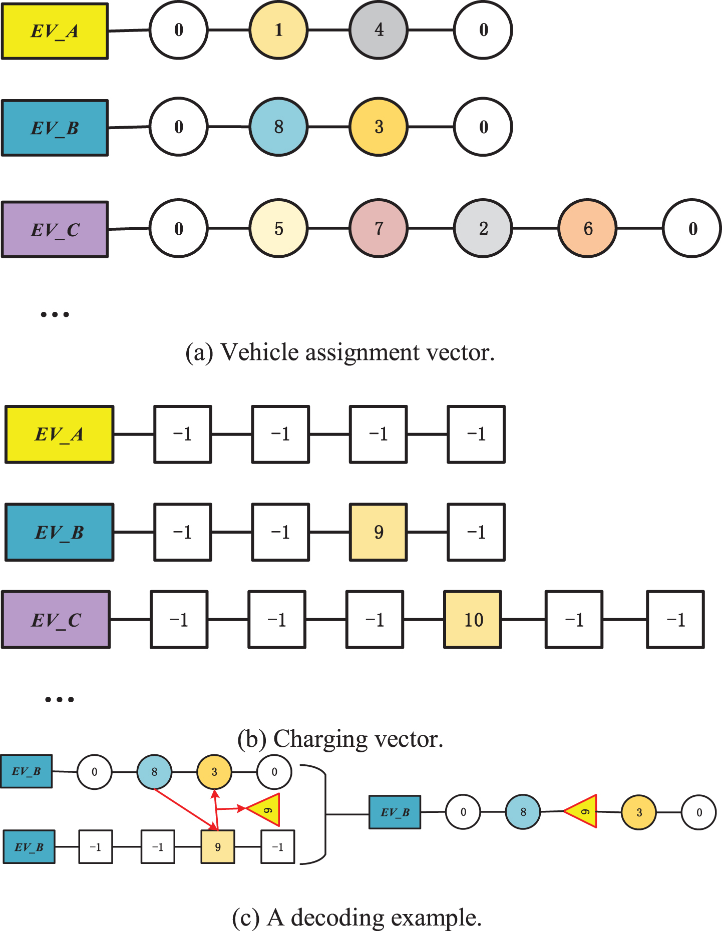
In this section, considering the problem constraints, two vectors are utilized to represent a solution, i.e., the vehicle assignment vector and the charging vector. The vehicle assignment vector is used to tell the assignment of the vehicles to each customer and provide sequence for the vehicle routes as well, and the charging vector tells whether a vehicle should be recharged at each charging station. Each vector contains a two-dimensional array. Figure 2(a) gives the illustrative example for the vehicle assignment vector, where the first dimension tells all the vehicles in the system and the second dimension represents the assigned customers for each vehicle. For example, there are three vehicles: the first vehicle serves two customers {1, 4}, and the other two vehicles serve {8, 3} and {5, 7, 2, 6}, respectively.

OPEN IN VIEWER

Fig. 2

Encoding representation and decoding.

Figure 2(b) tells whether a vehicle should be recharged at each charging station, where the element is set to the charging station number if the vehicle should be recharged at the corresponding charging station, otherwise, it is set to “–1”. For instance, the first vehicle will not visit any charging stations. The second vehicle will be recharged at the charging station numbered 9, while the last vehicle will be recharged at the charging station numbered 10.

In decoding procedure, first, it can use the charging vector to judge whether a vehicle recharged at the charging station, and then combine the vehicle assignment vector to determine the recharging operation between customers or between customer and depot, and finally find the entire route. In Fig. 2(c), two customers {8, 3} are served by the EV_B, the second sequence of {–1, –1, 9, –1} represents that the EV_B will be recharged at the charging station numbered “9”. It can be observed that the recharging operation between the customers numbered 8 and 3. Therefore, the entire route of the EV_B is expressed as {0, 8, “9”, 3, 0}.

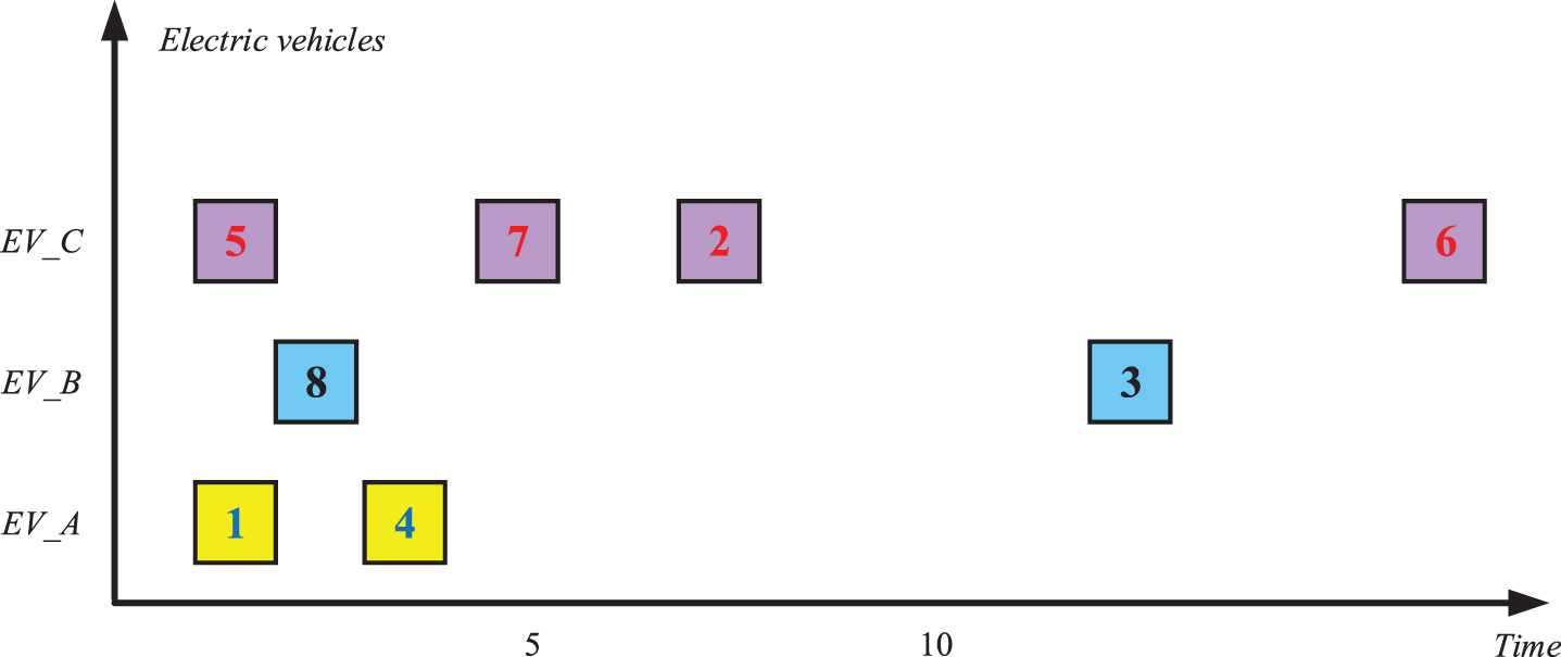
As mentioned above, the operations (like encoding, decoding, fitness evaluation) are illustrated as follows. Figure 3 presents a feasible Gantt chart. Each rectangle represents a customer. The customer parameters of the example (Fig. 1) are shown in Table 1. The vehicle assignment vectors and charging vectors are illustrated in Fig. 2. Without considering the battery capacity, the sequence of the EV_A is {1, 4}, the sequence of the EV_B is {8, 3}, and the sequence of the EV_C is {5, 7, 2, 6} (Fig. 2(a)). Then, prerequisites of battery capacity constraint is considered to the solution, to calculate the remaining battery capacity when the EV arrives at the customer. If the remaining battery capacity is negative, try inserting the charging station for recharging (that discussed in sub-section 4.3). Therefore, the charging vector is illustrated in Fig. 2(b). According to the Gantt chart, the trip time is obtained by the customer information and the charging time, and customer satisfaction level is calculated by the time windows and the time when the EV arrives at the customer. Consequently, the problem objective fitness is obtained by the weighted sum of the total trip time and customer satisfaction value.

4.3 The initialization strategy of charging stations

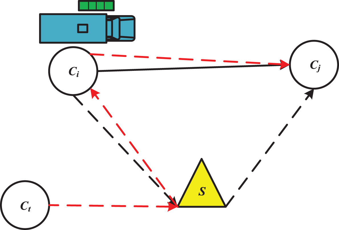
First, to assign the customers without considering the battery capacity, and then consider the prerequisites of battery capacity to the solution. It is necessary to record the battery consumption between customers and between customer and depot. Because some vehicles arrive at the customer, the remaining battery capacity may be negative. Therefore, it is necessary to consider inserting the charging stations for the charging operation. The example of inserting charging stations is illustrated in Fig. 4.

OPEN IN VIEWER

Fig. 3

Gantt chart of the example.

OPEN IN VIEWER

Fig. 4

The example of inserting charging station.

The number of negative remaining battery capacity represents s _n . The detailed steps of initialization strategy of inserting charging stations are given as follows:

To better understand the process of inserting charging stations, it can be described as follows. Before inserting into the charging station, the first step is to get the sum of the negative remaining battery capacity when the vehicle reaches the customer and the current trip time. If the remaining battery capacity is negative, it is necessary to try inserting the charging station for charging. To obtain an optimal solution, try inserting each charging station at each location. After charging, it needs to recalculate the total trip time and the negative remaining battery capacity.

If the negative value improves after inserting the charging station, there is still a negative battery capacity. Try considering inserting into other charging stations. After that, it could improve the negative remaining battery capacity.

Finally, after testing all charging stations for every location, select the best charging station to the best location for real insertion. The time complexity of the initialization strategy of charging stations is O (n³).

Recently, more and more people pay attention to the service performance. It can be reflected by customer satisfaction. The common approach to calculate it is considered as a linear function [53] and added it directly to the objective. However, customers usually cannot give an accurate satisfaction value in practice. The service satisfaction is assumed to be a piecewise function [54]. Figure 5 tells the piecewise function.

OPEN IN VIEWER

Fig. 5

Service-level function of time windows.

The approaches to calculate the customer satisfaction are as follows (t _i is time when the EV arrives at customer i):

When E _ti  ⩽ t _i  ⩽ L _ti , sv _i  = 1.

Each customer satisfaction level sv _i is obtained according to t _i (time when the EV arrives at customer i) and the time windows of each customer. The tolerate time is the same for every customer in this study, so the customer satisfaction value is converted into a uniform scale. The calculation of customer satisfaction value leverages the relationship of time (i.e., time when the EV arrives at customer i and the time windows of each customer) and the customer satisfaction value is between 0 and 1. For example, assuming that the time window is [E_ti, L _ti ] = [20, 40], the tolerance time is 5, i.e., [EE_ti, LL _ti ] = [15, 45] and t _i  = 43. The customer satisfaction level: sv i = ( 1 - 43 - 40 45 - 40 ) = 0.4 .

In the canonical DE algorithm, the mutation operator is to realize the individual mutation and generate the neighboring solution. However, it is used for continuous optimization problem. To better deal with this problem, the improved mutation heuristics is described as follows. There are two strategies for the current solution:

To generate neighboring solution, randomly chose one EV, and then one customer is randomly chosen from the chosen EV. Then, this customer is randomly removed from the newly chosen EV and inserted another EV to obtain a better solution. The time complexity of the first improved mutation heuristics is O (n²).

OPEN IN VIEWER

Fig. 6

Improved mutation process.

The detailed steps are given in the algorithm 3. It can be seen that the second method can generate a solution with more differences from the current one, and therefore can improve the detection abilities of the proposed algorithm.

In the canonical DE algorithm, the crossover operator is leveraged to solve continuous optimization problem. To better deal with this problem, the improved crossover operation is described as below. It randomly generates the newly solution through the crossover probability P _c . Figure 7 shows an example of the improved crossover operation. Two solutions are given in this figure: one is the current solution, and the other is the best solution. First, randomly select a vehicle from the current solution, find these customers who are served by this vehicle from the best solution, and then delete the corresponding customers from the best solution. At last, replace these deleted customers from the best solution and insert them into other vehicles to generate the crossover solution.

OPEN IN VIEWER

Fig. 7

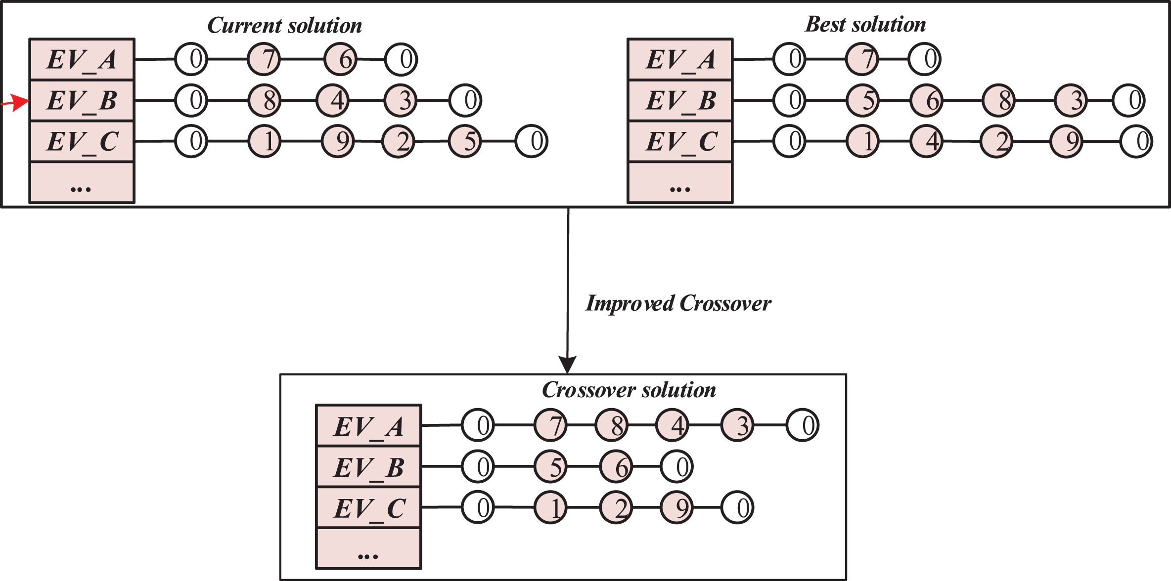
Crossover process.

The detailed steps of the improved following operation depicts in the algorithm 4. The time complexity of the improved crossover operation is O (n²). To ensure the non-negative battery capacity, it also continues to implement the charging station insertion strategy after the crossover operation.

Note that the current solution is to delete customers from the vehicle with the delete rate D _r .

In the current strategy, the EV is fully charged each time, but it still has the remaining battery capacity when it comes back to the depot. In terms of the concept of environmental protection, it is necessary to decrease the charging battery capacity. Therefore, a battery charging adjust (BCA) strategy is proposed in this paper. According to the last customer residual battery capacity, adjusting the charging battery capacity could decrease the total trip time.

The BCA strategy displays as below. First, record whether the charging operator is used for each vehicle. Then, remember the charging stations numbered for the next steps. Finally, recalculate the battery capacity and the charging battery capacity is set to the appropriate value. The time complexity of the BCA strategy is O (n²). It satisfied with the following conditions.

If there is only one charging station in the route, ensure that after charging in the current charging station, the vehicle returns to the depot with the zero remaining battery capacity.

4.8 Negative repair strategy

After the improved mutation operation or crossover operation, some customers could not satisfy the nonnegative battery capacity constraint. Therefore, the current solution becomes infeasible. Consequently, a negative repair strategy is proposed in this paper. There are two approaches to consider:

To generate a feasible solution, delete these customers with negative remaining battery capacity and add an extra vehicle to serve these customers.

The time complexity of the negative repair strategy is O (n²). It can use the figure to depict this process in detail. For example, delete the customer numbered 30 from the vehicle numbered 10. Now, assume insert into the ten vehicles (i.e., vehicles numbered 0 to 9), and the vehicle numbered 7 served these customers, including {1, 2, 5, 7}. There is a charging station numbered 8 between the customer numbered 5 and 7. The charging battery capacity is 100 in the charging process. It can increase 150 to ensure that this vehicle reaches the customer numbered 7 and then serves the customer numbered 30. The sequence can present {1, 2, 5, 7, 30} with the negative repair strategy (as shown in Fig. 8).

OPEN IN VIEWER

Fig. 8

Negative repair process.

With the above research, time complexity of the IDE algorithm is O (n³). Framework of the IDE algorithm is shown as below:

5.1 Experimental instances

The instances of this paper are generated from the Solomon benchmark instances. Clustering method is leveraged to divide the 100 customers of the Solomon instances into a number of categories by calculating the distance between each customer. Then, it designs the location of the charging station for each category by calculating the mean value of the customers’ coordinates which belong to each category. The instances can be found in the website"https://www.researchgate.net/publication/334735357_nonLinearVRPTWInstances". In reality, these midpoints may be more than or less than demand.

It contains 55 instances, named “c101” to “rc207”. Differences with the classical Solomon are listed below.

All EVs have a tripe of data, i.e., an energy consumption rate that tells the energy consumption for each unit of travel distance, a fixed capacity that represents the vehicle load capacity.

In this paper, the battery consumption is assumed to be equal to the distance on arc. The maximum battery capacity of the EV is 300.

5.2 Experimental parameter

To effectively set the system parameters, preliminary experiment is carried out. The parameters included in the experiment are as follows and shown in Table 2.

The population size P_s, which is the total number of individuals in an experiment.

In the DOE Taguchi method, an orthogonal array L₁₆ (4³) is leveraged [55]. The IDE algorithm was independently run 30 times with each parameter combination, and the average fitness value is used as the response variable (RV). Table 3 shows the results of various combinations of parameters. Figure 9 depicted the factor level trend.

OPEN IN VIEWER

Fig. 9

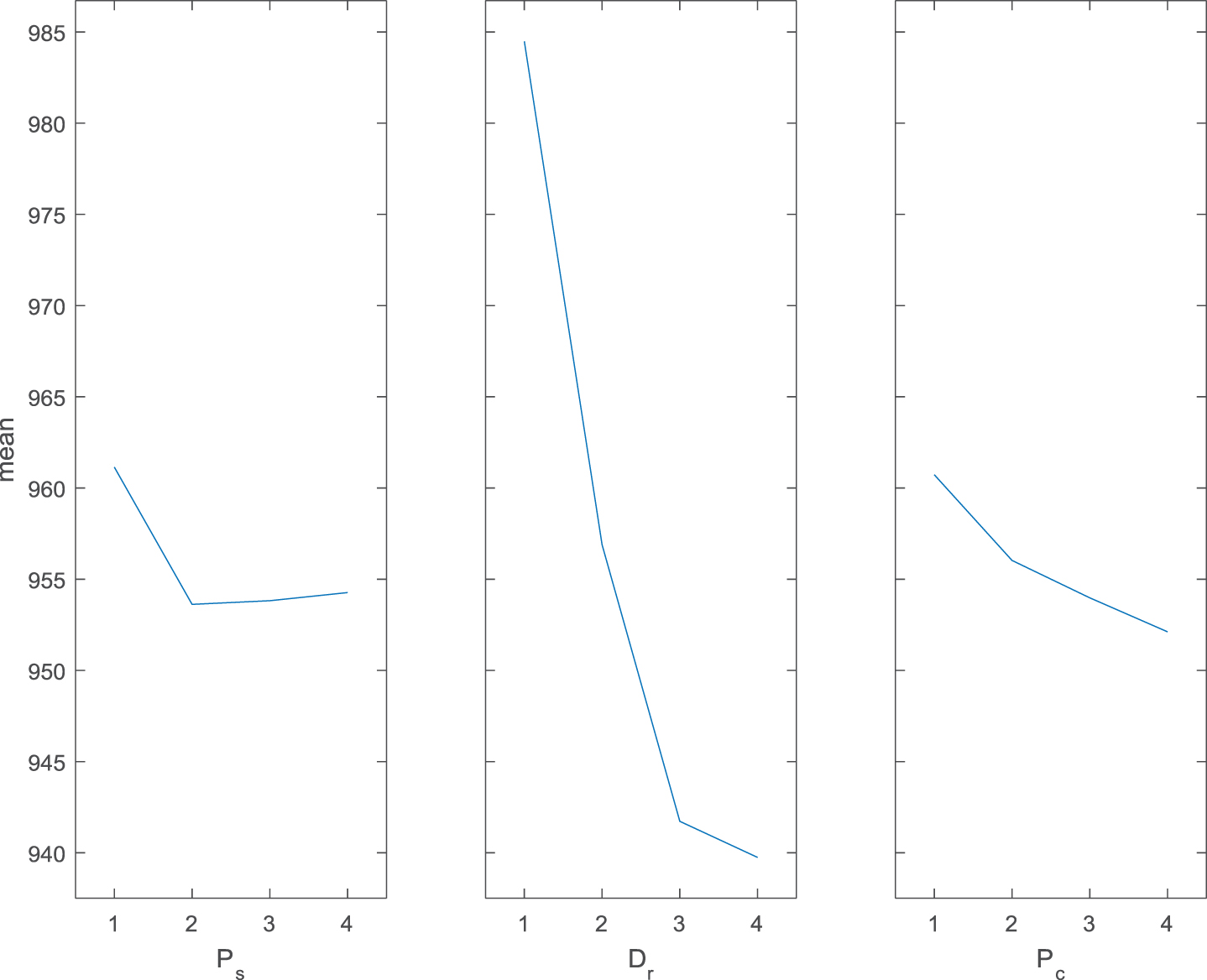
Factor level trend of three parameters.

As shown in Fig. 9, the IDE algorithm achieves better by selecting the following three key parameter levels: (1) P _s is the level 2; (2) D _r is the level 3; and (3) P _c is the level 4. Consequently, the suitable values of P _s , D _r and P _c are set to 100, 0.5 and 0.8, respectively.

In this section, to investigate the advantage of the improved crossover operator in this paper, it conducted a comparison with the classical crossover operator [44], i.e., the classical crossover operator (IDE-I for short), and the improved crossover operator (IDE-II for short). The fitness values obtained after 30 independent runs for 55 extending the VRPTW instances. Table 4 displays the experimental results.

It contains the instance name, the experimental results of the IDE-I and the IDE-II in minimum, average and maximum, respectively, and the percentage deviation. The calculation formula is given at (30): dev = ( f c - f b ) / f b × 100(30) As seen from Table 4, the IDE-II has the following features: (1) 39, 35, and 37 better values are obtained, while there are only 16, 20, and 18 better values calculated by the IDE-I in minimum, average and maximum, respectively; (2) as shown in the last line, the IDE-II obtains an average percentage deviation 0.58, 0.52, and 0.51. According to the table, the proposed crossover operator is significantly superior compared with the classical operator.

To further test whether the differences from the above table are significant, Fig. 10(a)-(c) conducted detailed comparisons. It presented the means and 95% LSD intervals for fitness with the IDE-I and IDE-II. It is obvious that the IDE-II presents superiority of statistical significance with respect to the IDE-I. This main reason for this results is that by using the improved crossover operator (i.e., the sub-section 4.6 discussed), the newly generated solution can boost seek and exploration capabilities.

OPEN IN VIEWER

Fig. 10

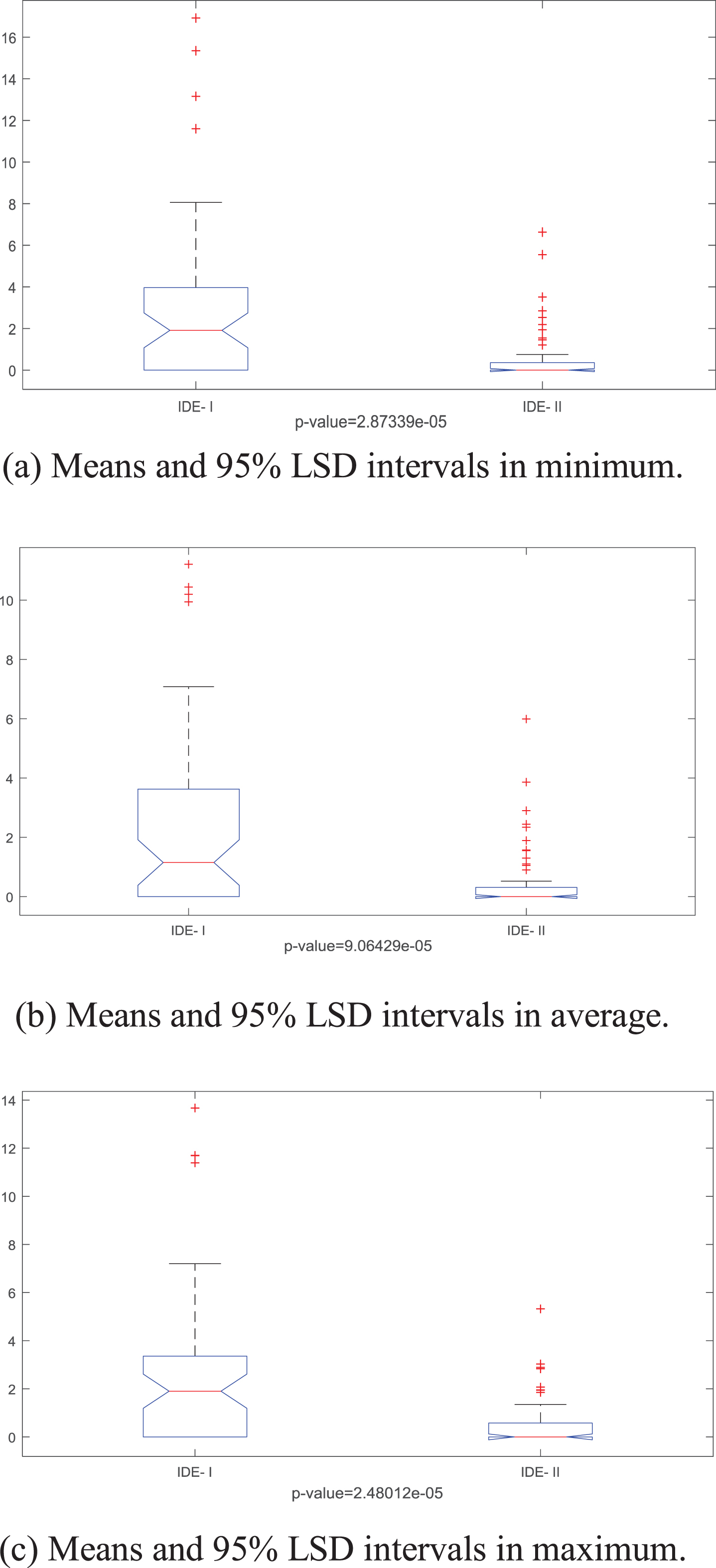
Means and 95% LSD intervals for IDE-I and IDE-II.

To further verify and test the validity of the IDE algorithm, the two-phase GA [30] and the improved TS algorithm (ITSA) [29] were selected as the comparison algorithms. The two-phase GA and the ITSA were efficient algorithms to solve a series of VRP. Likewise, the two algorithms can be applied to these instances for further comparison, re-encode the two-phase GA and ITSA aims to solve the EVRPTW-NL.

For experimental credibility, tested three algorithms on the same computer with the same 55 extended instances over 30 independent runs. The minimum and average values of these experiments are shown in the following two tables.

Table 5 shows the comparison experiment results: (1) 37 better solution are obtained by the IDE algorithm, while there is only 1 optimal solution calculated by the two-phase GA and 21 optimal solution calculated by the ITSA. (2) from the last line, the IDE algorithm obtains an average percentage deviation 1.11.

Table 6 presents that: (1) the IDE algorithm had 35 better values, while there are only 2 and 19 optimal solutions calculated by the two-phase GA and the ITSA respectively. (2) as shown in the last line, the IDE algorithm is 0.81.

The two tables show that the IDE algorithm is significantly superior in minimum and average than the other classical algorithms.

Figure 11(a)-(d) illustrates the two pairs of compared algorithms in minimize and average. The p-value is close to 0, indicating significant differences between the compared algorithms.

OPEN IN VIEWER

Fig. 11

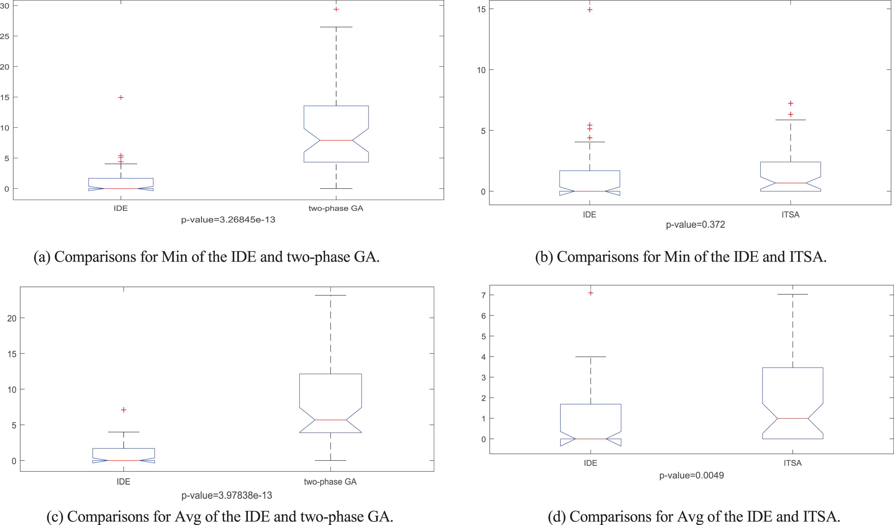
Means and 95% intervals for different algorithms.

To further verify the performance of the developed algorithm in solving this problem, randomly selected six instances ‘Inst1, Inst10, Inst18, Inst30, Inst41, Inst49’. Figure 12(a)-(f) reports the convergence curve of these instances, showing the effectiveness of the IDE algorithm.

OPEN IN VIEWER

Fig. 12

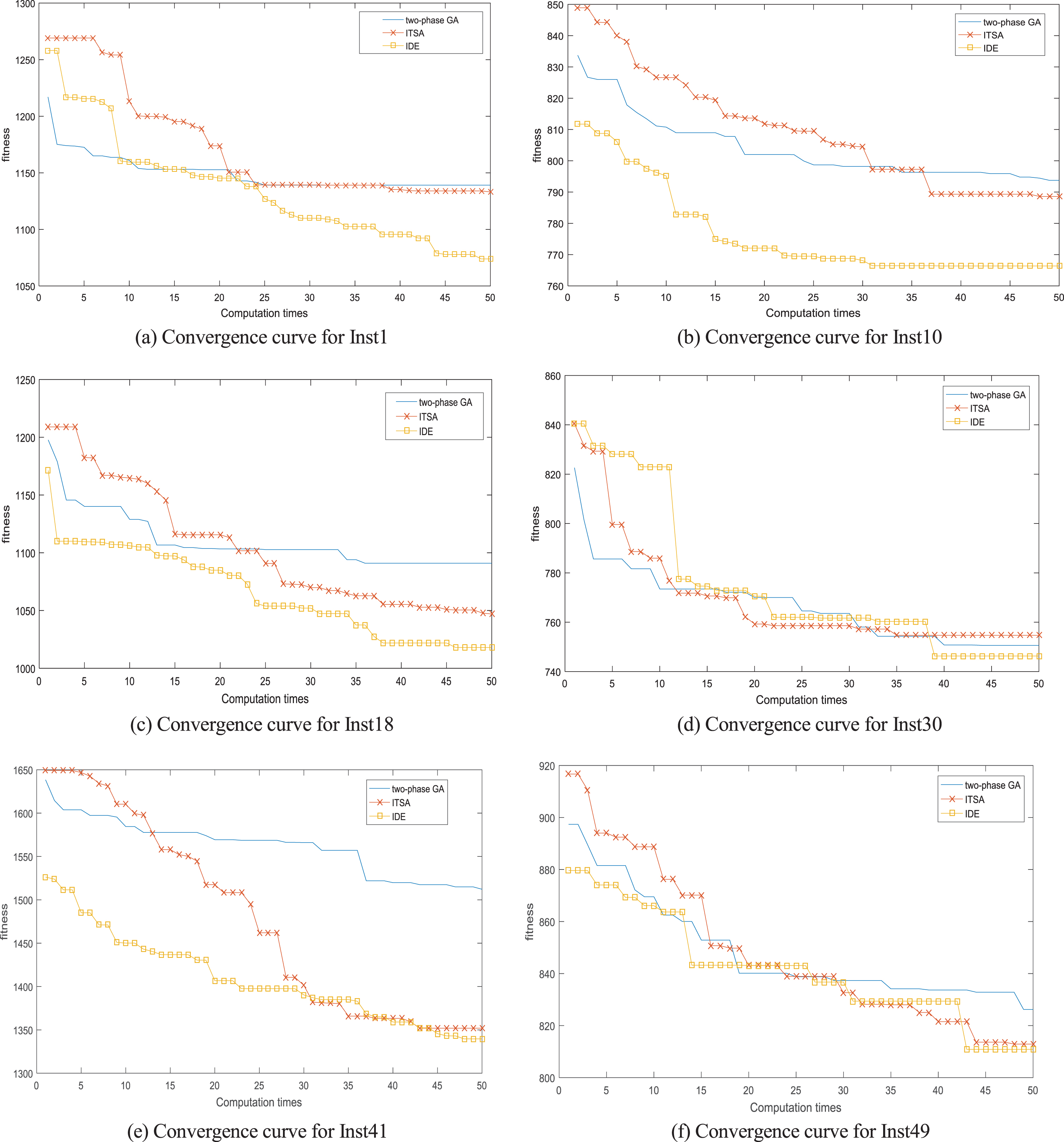
Convergence curve for instances.

Figure 13 presents the customer service time and charging time Gantt diagram of the instance. For example, the “V11” route is: V 11 : C 59 → C 58 → C 6 0 → ′ CS 3 ′ → C 38 → C 39 → ′ CS 1 ′ → C 19 → C 12 → C 1 00 . The total number of customers is 8. It is noticed that the “V11” charged in the charging station numbered 3 between customer 60 and 38. The figure shows the effectiveness of the IDE algorithm.

OPEN IN VIEWER

Fig. 13

Gantt chart for the instance.

As seen from the Equation (1), the weighted sum method is leveraged to calculate the objective fitness and the weight w is to optimize the two objectives, i.e., the total trip time and the customer satisfaction value sv _i . The weight w was set to 0.8 in this study. Reasonable weights are important for decision-making. In this section, we set the weight value to {0.1, 0.2, 0.3, 0.4, 0.5, 0.6, 0.7, 0.8, 0.9} to test the influence of each weight on the total trip time and customer satisfaction value. Each instance was run independently 10 times for ten instances. Figure 14 illustrates the results of the experiment, where each point represents the difference between the optimal objective value and the average objective value for each instance at the current weight value. It shows that: (1) the weight effects the balance between the total trip time and customer satisfaction value; (2) different weights have different optimization effects on the objective fitness.

OPEN IN VIEWER

Fig. 14

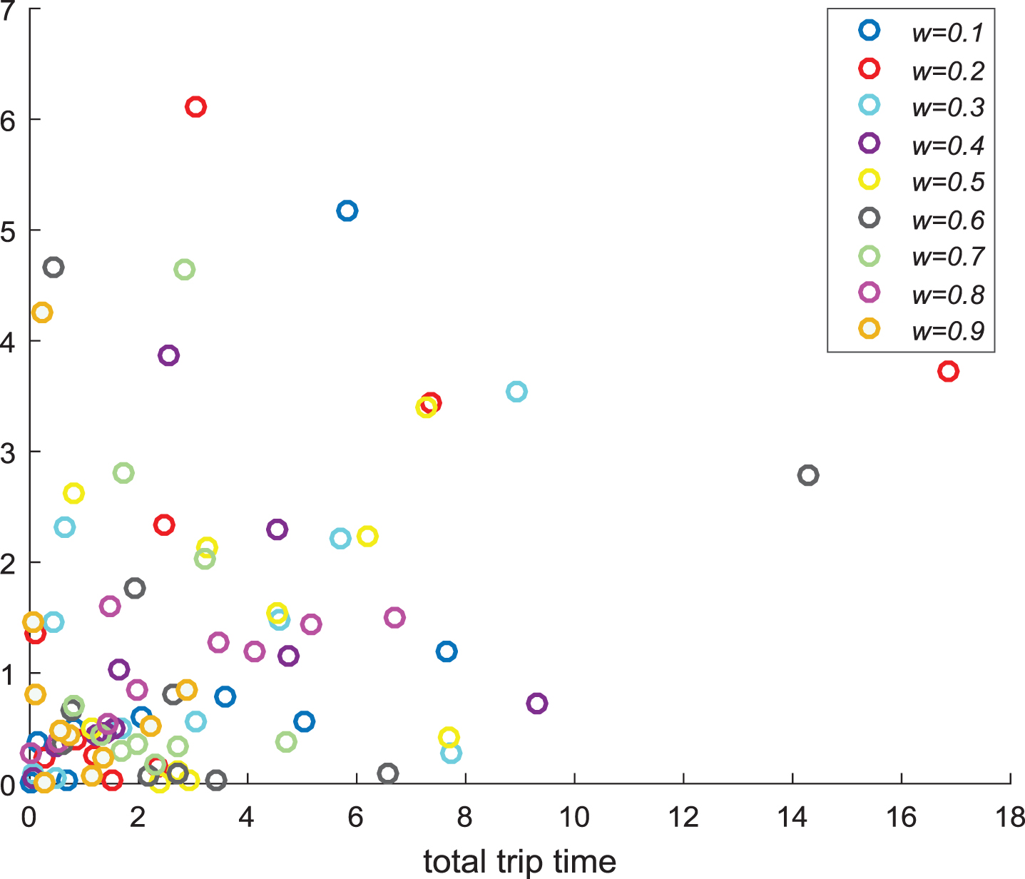
Comparison with different weights.