Adaptive scale weighted fuzzy C-Means clustering for the segmentation of purple soil color image

Abstract

The segmentation and extraction of the purple soil region from purple soil color image can effectively avoid the influence of background on recognition of soil types. A scale weighted fuzzy c-means clustering algorithm(SWFCM) is proposed for effective segmentation of purple soil color image. The main work is to establish the maximum difference optimization model with the mean of Gaussian distance between each pixel and each peak of the image histogram, and optimize the clustering number and the initial clustering centers. Then, the compactness of each class is defined to weight the Euclidean distance between the pixel and the clustering center and improve the optimization model of FCM for raising its clustering performance. Aiming at the problem of removing scattered small soil blocks in the background and filling holes in the purple soil region, the algorithm of extracting the boundary of the purple soil region and the algorithm of filling the purple soil region are proposed. Finally, the normal and robust experiments are carried out on the normal sample set and robust sample set. And the performances of relative algorithms are compared, which involves the previously released FCM algorithms and some methods for the segmentation of purple soil color image and our proposed algorithm. Experimental results show that performance of SWFCM is better and it can provide a high reference for adaptive segmentation of purple soil color images. Especially for robust experiment images, its average segmentation accuracy is improved by 6 . 64% ∼ 8 . 25 % compared with other purple soil segmentation algorithms.

Keywords

color image segmentation purple soil fuzzy c-means clustering(FCM)

1 Introduction

The cultivation of most crops is inseparable from soil and the high yield of crops is closely related to soil. With development of agricultural automation technologies, it is possible to recognize soil types by machine vision technology. Soil identification based on soil classification system is the basis of soil resources utilization and improvement, and it can provide scientific and technical support for improving soil fertility and formulating crop cultivation measures, so as to achieve the scientific development of agricultural production. But The classification of soil is complex, and traditional soil species identification is artificial identification of soil structure on natural soil faults, which only depends on the professional skills of soil experts. It even causes that many of ordinary agricultural scientists and technicians can not meet the requirements of accurately identifying soil types, and it is more difficult for ordinary agricultural practitioners [1]. In order to spread the technology of identifying soil types to farmers at the grass-roots level and realize more scientific agricultural production, the technology recognized soil types by machine vision has wide application and research value.

Purple soil is a kind of special soil and is widely distributed in Southwest China and there are rich nutrients in it. Under natural conditions in the field, a purple soil image obtained by machine vision inevitably contains complex backgrounds such as planted crops, mosses and weeds, which will interfere with the recognition of purple soil type. Therefore, segmenting and extracting the purple soil region image from the purple soil color image is the basic work for further identifying the purple soil types and analyzing the attribute value of the purple soil, and it is also the primary problem for studying the identification of purple soil types.

The segmentation of purple soil color image is a process of extracting an image of natural soil fault with intact soil structure. Accurate segmentation of purple soil color image is a challenging task due to the existence of shadows and the complex background and similar topsoil in it.

There are very few soil image processing documents that can be retrieved in nearly 10 kinds of mainstream Chinese and foreign literature databases. In the published literatures, threshold approaches and clustering approaches are mostly used. For the first time, Cheng(2019) [1] used normal distribution to fit the ’H’ component histogram of soil image and obtained the confidence interval of the ’H’ color component with 95% confidence as the segmentation threshold, but it is rather farfetched and the segmentation effect is poor due to poor fitting accuracy. In order to further improve the segmentation accuracy, the soil image was segmented by the improved simple linear iterative clustering algorithm (SLIC,2019) [2], and then the super-pixels belonging to the soil were merged. However, the disadvantage of this method is that it is unable to perform adaptive segmentation. Subsequently, Zeng(2019) [3] established an optimization model with the maximum ratio of inter-class variance and intra-class variance between soil and impurities in the purple soil region to optimize the confidence probability, and used Chebyshev inequality to acquire the segmentation threshold adaptively. It realizes the adaptive segmentation of soil image, but its segmentation accuracy needs to be improved.

To further improve the segmentation accuracy of purple soil color image, image segmentation algorithms in other fields are referenced. At present, neural network and deep learning are wildly used in the image segmentation and other field. However, because these algorithms require a large amount of data for training and it is expensive to collect soil images and number of the collected soil images is limited not to satisfy requirement of deep learning samples, they are not suitable for soil image segmentation. Fuzzy c-means clustering(FCM) has attracted our attention for segmenting soil image and it would be improved.

The rest of this paper is organized as follows. Section 2 reviews the FCM algorithms. SWFCM is described in Section 3. Section 4 shows the segmentation of purple soil color image. Experimental results are given in Section 5 and Conclusion of this paper is in Section 6.

2 Work related to FCM algorithm

FCM [4, 5] is a classical algorithm used in image segmentation because of its advantages such as better fault tolerance and retaining more original image information than hard clustering [6]. It was widely used in the segmentation of natural images [7 –9], medical images [10, 11] and remote sensing images [12, 13]. For the dataset X ={ x₁, x₂, . . . , x_n }, the FCM objective function is shown as Eq. (1). $\min J_{FCM} = \sum_{i = 1}^{n} \sum_{j = 1}^{C} u_{ij}^{m} {(x_{i} - v_{j})}^{2}$ (1) $s . t . \sum_{j = 1}^{C} u_{ij} = 1, 0 \leq u_{ij} \leq 1$ Here, C represents the number of clusters. v_j expresses the j^th center. u_ij denotes the fuzzy membership of x_i with respect to v_j. m is a weighting exponent to control fuzziness and 1 ≤ m ≤ 2.

Since FCM is sensitive to noise, some scholars integrate spatial neighborhood information into FCM to make it have better anti-noise capability [14], but it also brings high computational complexity at the same time. Then, FCM_S1 pre-integrates spatial neighborhood information into FCM by using average or median filtering to reduce time complexity [15]. The enhanced FCM algorithm (EnFCM) uses gray level instead of pixel to perform clustering, which further reduces the time complexity [16]. The EnFCM objective function is shown as Eqs.(2) and (3). $\min J_{EnFCM} = \sum_{i = 1}^{L} \sum_{j = 1}^{C} h (ξ_{i}) u_{ij}^{m} {(ξ_{i} - v_{j})}^{2}$ (2) $ξ_{i} = \frac{1}{1 + α} (x_{i} + \frac{α}{| N_{i} |} \sum_{r \in N_{i}} x_{r})$ (3) L represents the gray level of ξ_i, h (ξ_i) is the number of data points with value of ξ_i, ξ_i denotes the data value weighted by neighborhood information, α is the adjustment parameter, N_i is 3×3 neighborhood pixels centered on x_i, and |N_i| expresses the number of elements in the set N_i.

On the basis of EnFCM algorithm, the fast generalized FCM algorithm (FGFCM) [17] puts forward a new neighborhood information weighting method. The FGFCM objective function is shown as Eqs.(4)- (9). $\min J_{FGFCM} = \sum_{i = 1}^{L} \sum_{j = 1}^{C} h (ξ_{i}) u_{ij}^{m} {(ξ_{i} - v_{j})}^{2}$ (4) $ξ_{i} = \sum_{r \in N_{i}} s_{ir} x_{r} / \sum_{r \in N_{i}} s_{ir}$ (5) $a_{ir} = \max (| p_{i} - p_{r} |, | q_{i} - q_{r} |) / λ_{s}$ (6) $b_{ir} = {∥ x_{i} - x_{r} ∥}^{2} / λ_{g} σ_{i}^{2}$ (7) $s_{ir} = e^{- a_{ir} - b_{ir}}$ (8) $σ_{i} = \sqrt{\sum_{r \in N_{i}} {∥ x_{i} - x_{r} ∥}^{2} / | N_{i} |}$ (9) Where s_ir denotes the local similarity of space and color information, and (p_i, q_i) represents the coordinate of data point x_i in the image. λ_s and λ_g are the scale parameters of spatial and color information respectively.

To further improve anti-noise capacity, the neighbor weighted FCM algorithm (NWFCM) had defined the neighborhood-weighted distance to replace the Euclidean distance in the objective function of FCM based on image patches and local statistics [18]. NWFCM is able to provide better segmentation results for images corrupted by Salt & Pepper and Uniform noise, but it is sensitive to Gaussian noise. The NWFCM objective function is shown as Eqs.(10)- (14). $\min J_{NWFCM} = \sum_{i = 1}^{n} \sum_{j = 1}^{C} u_{ij}^{m} d_{N}^{2} (x_{i}, v_{j})$ (10) $d_{N} (x_{i}, v_{j}) = \sum_{r \in N_{i}} ω_{ir} \sum | x_{r} - v_{j} |$ (11) $a_{ir} = \exp (- {∥ G_{σ} * (N_{i} - N_{r}) ∥}^{2} / α σ_{i}^{2})$ (12) $b_{ir} = - {∥ G_{σ} * (N_{i} - N_{r}) ∥}^{2} / α σ_{i}^{2}$ (13) $ω_{ir} = a_{ir} / \sum_{r \in N_{i}} \exp (- b_{ir})$ (14) Where G_σ donates Gaussian template and σ_j is the same as Eq. (9).

The fast and robust FCM algorithm (FRFCM) is more robust to different noise than NWFCM because it incorporates the local spatial information of an image into FCM by introducing morphological reconstruction operation [19]. The FRFCM objective function is shown as Eqs.(11) and (12). $\min J_{FRFCM} = \sum_{i = 1}^{L} \sum_{j = 1}^{C} h (ξ_{i}) u_{ij}^{m} {∥ ξ_{i} - v_{j} ∥}^{2}$ (15) $ξ = R_{R_{f}^{γ} (ϑ (f))}^{ϑ} (γ (R_{f}^{ϑ} (ϑ (f))))$ (16) Where f is an original image, γ represents expansion operation, and ϑ donates corrosion operation. $R_{f}^{ϑ} (g) = ϑ_{f}^{(k)} (g)$ , $ϑ_{g}^{(k)} = ϑ$ (ϑ^(k-1) (g)) ∨ f, $ϑ_{f}^{(1)} (g) = ϑ (g) \lor f$ , $R_{f}^{γ} (g) = γ_{f}^{(k)}$ (g), $γ_{g}^{(k)} = γ (γ^{(k - 1)} (g)) \land f$ , $γ_{f}^{(1)} (g) = γ (g) \land f$ . g is a marker image. ∧ and ∨ mean to take the minimum and maximum value.

3 Improving FCM

Aiming at its poor segmentation effect for purple soil color image and initializing manually the clustering centers, FCM algorithm will be improved. The FCM improvements based our works include two parts: 1) Initializing adaptively the clustering centers. 2) Considering the influence of the clustering compactness on the effective classification of boundary points, a clustering compactness measure is defined and integrated into the traditional FCM algorithm by weighting.

3.1 Initializing the clustering centers

Initializing a suitable clustering centers not only helps to speed up the stability of the clustering centers, but also provides a better result for data classification. Therefore, an algorithm for initializing the clustering centers is designed. Due to the high density of the main peak of data histogram and the data points distributed around it, main peaks of the data histogram are usually initialized as the clustering centers [20]. By observing the ’a’ component histogram of 60 color images of purple soil, it is found that the main peaks have the following characteristics.

1) the density of the main peak and its surrounding distribution points is high.

2) There is a certain distance between two main peaks.

To meet the first characteristic mentioned above, the mean of the Gaussian distance (MGD) is introduced to reflect the density of the main peak and its surrounding points. Before calculating the MGD, all the peaks in histogram are first calculated, as shown in Eqs.(13)-(15). $h (l) = \sum_{i = 1}^{n} sign (x_{i} - l)$ (17) $sign (Z) = {\begin{matrix} 1, Z = 0 \\ 0, others \end{matrix}$ (18) $p e a k = {l | h (l) \geq h (l + 1) & h (l) \geq h (l - 1)}$ (19) Where n denotes the number of points. x_i is the i^th point. h (l) represents the number of points that its value is l, l ∈ [min (X) , max (X)].

Then, the calculation of MGD_j depends on the average difference between all points and the peak, as shown below.

${MGD}_{j} = \frac{1}{n} \sum_{i = 1}^{n} e^{- {(x_{i} - pea k_{j})}^{2} / 2 θ^{2}}$ (20) Where MGD_j represents the Gaussian distance mean of the j^th peak. peak_j denotes the j^th peak required by Eq. (15), j = 1, . . . , P. P is the total number of peaks. θ is the scale parameter of the Gaussian function. The term e^{-(x_i-peak_j)²/-2θ²} is intended to consider the difference between x_i and peak_j. The greater the density of peak_j and its surrounding points, the greater the value of MGD_j. That is to say, the peak peak_j corresponding to the larger MGD_j value can represent the clustering center. In order to determine the clustering centers, the parameter ɛ is obtained to dichotomize the set D ={ MGD₁, . . . , MGD_P } (the selection of ɛ is obtained in section 3.2). As shown in Eq. (17), the peak peak_j satisfied MGD_j ≥ ɛ can represent a clustering center, while the peak peak_j satisfied MGD_jlessɛ is a pseudo peak.

$V = {pea k_{j} | {MGD}_{j} \geq ɛ, j = 1, . . ., P}$ (21) Here, although the set V satisfies the first characteristic mentioned above, it can not meet the second characteristic. In response to this question, the distance between two clustering centers being in one dimensional space can be measured by the Manhattan distance, which is the least computational effort. Next, to keep a certain distance between the clustering centers, it is required that the Manhattan distance between two adjacent clustering centers is less than the threshold ψ (show in Eq. (18)). If this is not satisfactory, v_k+1 is deleted from V.

$| v_{k} - v_{k + 1} | less ψ, k = 1, . . ., Q$ (22) Where v_k is the k^th element in the ordered ascending set V. Q denotes the total number of elements in the set V.

3.2 Getting parameter ɛ

In the process of initializing clustering centers, the number of initial clustering centers is determined by the parameter ɛ. While ɛ is set to be larger, some main peaks in the set peak will be deleted. On the contrary, some pseudo peaks in the set peak can not be effectively deleted. In order to get a reasonable parameter ɛ, the maximum difference optimization model is raised. From the description in section 3.1, we know that compared with the MGD value of the main peak, the MGD value of the pseudo peak is very small. Therefore, the parameter ɛ can be obtained by maximizing the inter-class difference between the main peak set and the pseudo peak set. The specific steps are as follows. The mean value of all elements in the set MGD is first calculated, then delete the pseudo peaks whose MGD value is less than the mean value and keep the peaks whose MGD value is greater than the mean value from the set peak, and repeat the above steps. When the MDG mean difference of all elements in the set peak before and after deletion is the largest, the inter-class difference between the main peak set and the pseudo peak set can be maximized. At this time, the MDG mean value before deletion is set as the parameter ɛ. For the data D ={ MGD₁, . . . , MGD_P }, the mathematical model of the above optimization algorithm is shown as Eqs.(19) and (20). $ɛ = \underset{av g^{t}}{arg max} | av g^{t + 1} - av g^{t} |$ (23) $av g^{t} = \frac{1}{| D^{t} |} \sum_{MG D_{k} \in D^{t}} MG D_{k}$ (24) Where |D^t| is the number of elements in the set D^t, D^t ={ MGD_k|MGD_k ≥ avg^t-1, MGD_k ∈ D^t-1 }. Note that D⁰ = D. avg^t denotes the mean of all elements in the set D^t.

The procedure of getting parameter ɛ is summarized as Algorithm 1.

Algorithm 1 Getting parameter ɛ

Require: The set D and peak.

Ensure: The parameter ɛ.

1: Compute the mean value avg⁰ of the set D.

2: Delete the peaks whose MGD value is less than avg⁰ from peak.

3: Set D¹ ={ MGD_k|MGD_k ≥ avg⁰, MGD_k ∈ D }, t = 1, mind = 0.

4: repeat

5: Compute the mean value avg^t of the set D^t.

6: Delete the peaks whose MGD value is less than avg^t from peak.

7: Compute d = |avg^t+1 - avg^t|.

8: if dgreatermind then

9: Set mind = d and ɛ = avg^t.

10: end if

11: Update D^t+1 ={ MGD_k|MGD ≥ avg^t, MGD_k ∈ D^t }.

12: Set t = t + 1.

13: until (there is only one element in the set peak)

3.3 Scale weighted fuzzy c-means clustering algorithm (SWFCM)

In FCM, the classification of point x_i is simply determined by the distance between x_i and each center. This strategy is effective for the classification of the points close to one clustering center and far away from other clustering centers, but it can not provide a good effect for the classification of the points at the junction of two clusters.

For example, as shown in Figure 1, there are two clusters with different dispersions, and there is an unlabeled red point at the junction of the two clusters. According to the FCM algorithm, the probability of the red point belonging to the cluster A is higher, because it is closer to the center of the cluster A. However, it has a greater impact on the intra-class variance of the cluster A than that of the cluster B, which obviously violates the clustering criterion of minimizing the intra-class variance and maximizing the inter-class variance.

Fig. 1

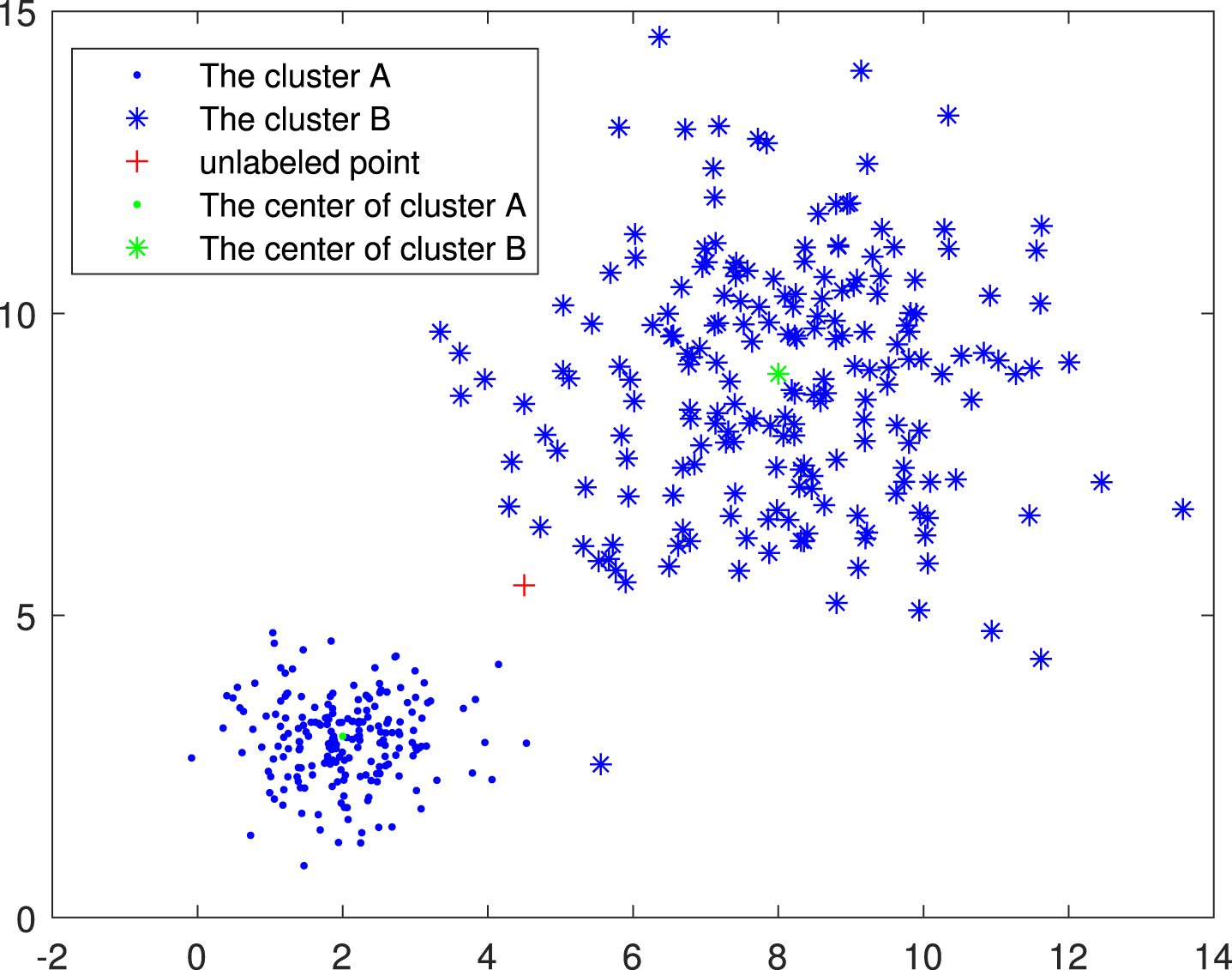
The scatter diagram of two clusters.

Aiming at the defect that FCM can not provide a good performance for the classification of the points at the junction of two clusters, the compactness of clusters is defined to weigh the Euclidean distance between point and the clustering center, so that the points at the junction of two clusters are more likely to belong to the cluster with smaller compactness. The objective function of the improved FCM is shown in Eq. (21). $\min J_{SWFCM} = \sum_{i = 1}^{n} \sum_{j = 1}^{C} u_{ij}^{m} ω_{j} {(x_{i} - v_{j})}^{2}$ (25) $s . t . \sum_{j = 1}^{C} u_{ij} = 1, 0 \leq u_{ij} \leq 1$ Here, ω_j (0lessω_jless1) is interpreted as the compactness of the j^th cluster and computed by Eq. (22). From Eq. (26), it can be seen that the fuzzy membership u_ij is not only controlled by the distance between the point x_i and the clustering center v_j but also affected by the compactness of the j^th cluster. When the distance between the point x_i and two clustering centers is equal, the probability that this point belongs to the cluster with small compactness (u_ij) is high.

The compactness ω_j is defined by calculating the reciprocal of the dispersion σ_j of the j^th cluster, and then normalize it to [0,1]. The mathematical expression of ω_j is shown in Eq. (22).

$ω_{j} = \frac{1}{σ_{j}} / \sum_{k = 1}^{C} \frac{1}{σ_{k}}$ (26) Where σ_j expresses the dispersion of the j^th cluster. It is usually defined by the weighted average of the distances between all points and the clustering center. However, as shown in Figure 1, the dispersion of the cluster A is smaller than that of the cluster B, and the dispersion of two clusters calculated by the above method may be equal. In order to distinguish, we multiply the distance between point and the clustering center by the weighting coefficient, which requires that the distance weighting coefficient of points closer to the clustering center is larger, and conversely, the distance weighting coefficient of points farther away from the clustering center is smaller. In t^th iteration, the mathematical expression of σ_j is shown in Eq. (23). $σ_{j}^{(t)} = \sqrt{\sum_{i \in {CL}_{j}^{(t)}} ϖ_{ij}^{(t)} {(x_{i} - v_{j})}^{2} / \sum_{i \in {CL}_{j}^{(t)}} ϖ_{ij}^{(t)}}$ (27) $ϖ_{ij}^{(t)} = e^{- | x_{i} - v_{j} | / σ_{j}^{(t - 1)}}$ (28) Here, ${CL}_{j}^{(t)}$ represents the location set of the data points belonging to the j^th cluster after the t^th iteration. $ϖ_{ij}^{(t)}$ is the distance weighting coefficient between the point x_i and v_j.

Using Lagrange multiplier method [21], the objective function of SWFCM is equivalently transformed to Eq. (25). $\begin{matrix} \min J_{SWFCM} = & \sum_{i = 1}^{n} \sum_{j = 1}^{C} u_{ij}^{m} ω_{j} {(x_{i} - v_{j})}^{2} \\ + λ_{i} (\sum_{j = 1}^{C} u_{ij} - 1) \end{matrix}$ (29) Calculating the derivatives of J_SWFCM with respect to u_ij and v_i respectively and setting them to 0, this iterative formulas are obtained as Eqs.(26) and (27). $u_{ij} = {(ω_{j} {(x_{i} - v_{j})}^{2})}^{\frac{- 1}{m - 1}} / \sum_{k = 1}^{C} {(ω_{k} {(x_{i} - v_{k})}^{2})}^{\frac{- 1}{m - 1}}$ (30) $v_{j} = \sum_{i = 1}^{n} u_{ij}^{m} x_{i} / \sum_{i = 1}^{n} u_{ij}^{m}$ (31) To obtain stable U ={ u_ij|1 ≤ j ≤ n, 1 ≤ i ≤ C } and V ={ v₁, . . . , v_C }, Eqs.(26) and (27) are repeatedly implemented until the change of each clustering center is less than a threshold δ or the number of iterations T is terminated.

According to the above description, the procedure of the SWFCM algorithm is summarized as Algorithm 2.

Algorithm 2 The SWFCM algorithm

Require: An image imgA with size M × N.

Ensure: V and U.

1: Set ψ = 1,m = 2,δ = 0.5,T = 100.

2: Calculate the set peak of imgA by Eqs.(13)-(15).

3: Compute the set D by Eq. (16).

4: Getting ɛ using algorithm 1.

5: Initialize V⁽⁰⁾ and C by Eqs.(17) and (18).

6: Initialize Δ⁽⁰⁾ = { σ_i } _1×C, σ_i = 1/C and W⁽⁰⁾ = { ω_i } _1×C, ω_i = C, i = 1, . . . , C.

7: Set t = 1.

8: repeat

9: Update U^(t) using V^(t-1) and W^(t-1) by Eq. (26).

10: Update V^(t) using U^(t) by Eq. (27).

11: Update Δ^(t) using V^(t) and Δ^(t-1) by Eq. (23).

12: Update W^(t) using Δ^(t) by Eq. (22).

13: Set t = t + 1;

14: until (t ≥ T ∥ |V (t) - V (t - 1) | < δ)

3.4 Time complexity analysis

The time complexity of SWFCM is composed of two main parts. One is the initialization of clustering numbers and centers and its most time-consuming step is to count the peak, which needs to traverse all the pixels in the image. Its time complexity is O (M × N). The other is the clustering part. Its most time-consuming step is to update the membership matrix U. Iteration is executed T times in the worst case (the maximum number of iterations is T) and the distances between all pixels in the image and different clustering centers are calculated in each iteration. The iteration is executed once in the best case. So the average time complexity of the clustering part is O (T × M × N × C). Based on the analysis above, the average time complexity of SWFCM is O (M × N + T × M × N × C).

The time complexity of different algorithms is given in Table 1. Where M × N is the size of an image. C represents the clustering number. G denotes the gray levels of an image. S is the size of the filtering window. According to Table 1, EnFCM, FGFCM and FRFCM have low time complexity at the clustering part because G is much less than M × N. However, the time complexity of preprocessing (such as determining the optimal classification number) is lower than comparative algorithms (smoothing filtering, etc.)

Table 1
Time complexity of six improved FCM algorithms

Algorithms Time complexity

FCM_S1 O (M × N × S² + T × M × N × C)

EnFCM O (M × N × S² + T × G × C)

FGFCM O (M × N × S² + T × G × C)

NWFCM O (M × N × (S + 1) ² + T × M × N × C)

FRFCM O (M × N × S² + T × G × C)

SWFCM O (M × N + T × M × N × C)

Algorithms	Time complexity
FCM_S1	O (M × N × S² + T × M × N × C)
EnFCM	O (M × N × S² + T × G × C)
FGFCM	O (M × N × S² + T × G × C)
NWFCM	O (M × N × (S + 1) ² + T × M × N × C)
FRFCM	O (M × N × S² + T × G × C)
SWFCM	O (M × N + T × M × N × C)

4 Segmentation of purple soil color image

In this section, the segmentation of purple soil color image is introduced. It includes three steps: 1) Initial segmentation based on SWFCM. 2) Extracting boundary of the purple soil region. 3) Filling the purple soil region. Among them, the first step is used to extract purple soil region, and the last two steps are post-processing, mainly to ensure the integrity of purple soil region and removes impurities in the background. Figure 2 is a process result diagram of purple soil segmentation.

Fig. 2

Example of segmentation result. (a) A purple soil color image. (b) Segmentation result of Figure 2(a) with SWFCM. (c) The result of boundary extraction. (d) The result of Filling purple soil region.

4.1 Initial segmentation based on SWFCM

In previous research on segmentation of purple soil color image, Cheng and Zeng used the ’H’ color component to segment. Through histogram analysis, it is found that the ’H’ component of purple soil is distributed at both ends of the histogram for some purple soil color images (as shown in the Figure 3(d)). The reason is that the distribution model of ’H’ color component is a closed circle, and its value range is [0,360], while the ’H’ component of purple soil in some images is distributed in the range of [0,90] and [270,360] (as shown in the Figure 3(a)). Therefore, the ’H’ component is not suitable to segment all purple soil color images.

Fig. 3

Histogram analysis of the purple soil and background. (a) Distribution model of the ’H’ color component. (b) A purple soil color image. (c) The Ground truth of Figure 3(b). (d) The ’H’ component histogram of Figure 3(b). (e) The ’a’ component histogram of Figure 3(b).

In order to segment purple soil color image more effectively, the color components with significant differences between the background and the purple soil are selected through histogram analysis in different color space. A result of analysing the histogram of sixty images shows that there is the difference distribution between the purple soil region and the background on the ’a’ component (show in Figure 3(e)). Thus, we select the ’a’ component as the color feature of purple soil color image for segmentation. The procedure of segmenting purple soil color image based on SWFCM is summarized as Algorithm 3.

Algorithm 3 The segmentation of purple soil color image based on SWFCM

Require: A purple soil color image imgA with size M × N.

Ensure: The matrix matB.

1: Set a zero matrix matB with size (M + 2) × (N + 2).

2: Compute the ’a’ color component matA of imgA;

3: Getting V and U using matA by Algorithm 2.

4: Randomly capture five 50×50 windows from the 100×100 window centered on the center of matA, then remove the windows with maximum and minimum ’a’ component mean, and finally calculate the ’a’ component mean avgA of the remaining three windows.

5: The class element whose cluster center is closest to avgA is extracted, and the pixel value at the corresponding position in matB is set to 1.

4.2 Extracting boundary of purple soil region

The boundary extraction of purple soil region can be realized by obtaining the boundary which has the largest area enclosed by it and contains the center of image. As shown in Figure 4(a), it is a binary matrix matB that simulates the image result after initial segmentation. The pixels with value of 1 represent purple soil, and the pixels with value of 0 represent background. Figure 4(b) shows the process of purple soil boundary extraction. Firstly, keeping the center of matB unchanged, the size of matB is expanded from M × N to (M + 2) × (N + 2). The pixel value of expanded part of imgB is set to 0. Secondly, starting from the center point of matB, the point with value of 0 is searched towards the right as the boundary starting point bsp. Thirdly, bsp is initialized as the current point cp and its left neighborhood point is initialized as the initial search neighborhood point isnp. In the four neighborhood points of cp, the first point fp with a value of 0 is searched counterclockwise starting from isnp (If there is no point with value of 0 in the four neighborhoods of cp, so the point cp is an isolated point, and then we search for the next boundary starting point starting form bsp). Then, isnp is updated with cp, and cp is updated with fp. According to the above rules, isnp and cp are updated repeatedly, and the coordinate position of cp is recorded in the matrix edg until cp returns to the position of bsp. Finally, it is judged whether the boundary formed by all current points contains the center of image. If so, this boundary is the boundary of purple soil, otherwise, the next boundary starting point is searched. The algorithm of extracting the boundary of the purple soil region is shown as Algorithm 4.

Algorithm 4 The algorithm of extracting boundary of the purple soil region

Require: The binary matrix imgB.

Ensure: The boundary matrix edg.

1: Initialize a zero matrix edg with size (M + 2) × (N + 2), dx ={ 0, 1, 0, - 1 } and dy ={ - 1, 0, 1, 0 }.

2: Keeping the center of imgB unchanged, imgB is expanded from M × N to (M + 2) × (N + 2). where the pixel value of expanded part of imgB is set to 0.

3: Set the center point of imgB to the current point (x, y).

4: repeat

5: Set y = y + 1.

6: if in the matrix imgB, the values of the neighboring points of the current point are different from its value then

7: execute step 5.

8: else

9: execute step 11.

10: end if

11: Set up = low = M/2, right = left = N/2, tx = x, ty = y, edg (tx, ty) = 1, i = 0 and initialize an empty stack stackA, push the current point (x, y) into it.

12: repeat

13: Initialize flag = 4.

14: repeat

15: Set i = (i + 1) % 4.

16: if imgB (tx + dx (i) , ty + dy (i)) = =1 then

17: Set flag = flag - 1.

18: else

19: Set flag = 0.

20: end if

21: until (flag = =0)

22: Set tx = tx + dx (i) and ty = ty + dy (i)

23: Set edg (tx, ty) = 1 and push (tx, ty) into stackA.

24: if i + 2 ≥4 then

25: Set i = (i + 2) % 4.

26: else

27: Set i = i + 2.

28: end if

29: if tx < M/2 then

30: Set up = tx.

31: else

32: Set low = tx.

33: end if

34: if ty < N/2 then

35: Set left = ty.

36: else

37: Set right = ty.

38: end if

39: until (tx = = x & ty = = y)

40: if low < M/2 < up & left < N/2 < right then

41: Pop all element (tx, ty) from stackA and set edg (tx, ty) = 0

42: end if

43: until (low < M/2 < up & left < N/2 < right)

4.3 Filling purple soil region

Figure 4(c) shows the process of filling purple soil region. The center of matrix edg is pushed into stackA. Starting from a point popped from stackA, horizontal search in edg is done along the left and right directions until a point with value of 1 is found at each direction. In the horizontal search, the points with value of 0 are pushed into stackB and their values in edg are set to 1. Then, starting from a point popped from stackB, longitudinal search in edg is done along the top and bottom directions until a point with value of 1 is found at each direction. In the longitudinal search, the points with value of 0 are pushed into stackA and their values in edg are set to 1. These two steps are repeated until both stackA and stackB are empty and the work of filling the purple soil region is finished. The algorithm of filling the purple soil region is shown as Algorithm 5.

Algorithm 5 The algorithm of filling the purple soil region

Require: The purple soil color image imgA, the binary boundary matrix edg.

Ensure: The purple soil region image.

1: Initialize a zero matrix matC and two empty stack stackA and stackB.

2: Push the center point of matrix edg into stackA.

3: repeat

4: repeat

5: Pop an element from stackA as the current point (x, y).

6: Set na = y - 1, nb = y + 1, edg (x, y) = 1 and matC (x - 1, y - 1) = 1.

7: repeat

8: if edg (x, na) = =0 then

9: Set matC (x - 1, na - 1) = 1, edg (x, na) = 1 and push (x, na) into stackB.

10: end if

11: if edg (x, nb) = =0 then

12: Set matC (x - 1, nb - 1) = 1, edg (x, nb) = 1 and push (x, nb) into stackB.

13: end if

14: Set na = na - 1 and nb = nb + 1.

15: until (edg (x, na) = =1 & edg (x, nb) = =1)

16: until (stackA is empty)

17: repeat

18: Pop an element from stackB as the current point (x, y).

19: Set na = x - 1, nb = x + 1, edg (x, y) = 1 and matC (x - 1, y - 1) = 1.

20: repeat

21: if edg (na, y) = =0 then

22: Set matC (na - 1, y - 1) = 1, edg (na, y) = 1, push (na, y) into stackA.

23: end if

24: if edg (nb, y) = =0 then

25: Set matC (nb - 1, y - 1) = 1, edg (nb, y) = 1 and push (nb, y) into stackA.

26: end if

27: Set na = na - 1 and nb = nb + 1.

28: until (edg (na, y) = =1 & edg (nb, y) = =1)

29: until (stackB is empty)

30: until (stackA and stackB are both empty)

31: The result of Hadamard product between matrix matC and the RGB three channels of imgA is the purple soil region.

Fig. 4

Example of post-processing algorithms. (a) The matrix matB. (b) Boundary extraction. (c) Filling purple soil region

4.4 Time complexity analysis

The initial segmentation of purple soil color image is based on SWFCM, so its time complexity is the same as SWFCM. The most time-consuming step of algorithm 4 is to traverse the boundary of the purple soil region, and it needs to traverse the boundary pixels of the purple soil region image and its four neighborhoods in the worst case. Thus its time complexity is O (M × N). The main step of algorithm 5 is to traverse the pixels in the purple soil region, which needs to traverse the whole image in the worst case. So its time complexity is O (M × N).

5 Experiments

Three experiments were done to verify the effectiveness of the proposed algorithm. Experiments include: 1) Evaluating the effectiveness of initializing the clustering centers. 2) Comparison of segmentation results with different FCM algorithms. 3) Comparison of segmentation results with other algorithms for the segmentation of purple soil color image.

Experimental environment is a graphic workstation with Intel(R) Xeon(R) CPU E5-2687W v2 @ 3.40GHz(2 CPU), 64 GB RAM and NVIDIA Quadro K5000 graphic card, and Visual Studio 2017.

5.1 Acquiring images

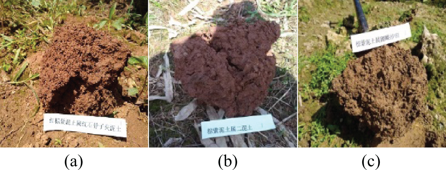
According to classification and code for Chongqing soil [DB50 / T 796-2017] [22], there are four soil genus and 34 soil types of purple soil at Chongqing, China. The natural fault of purple soil (core soil) is obtained by a spade in 0-25cm tillage soil, and it keeps the original features of purple soil. In order to extract purple soil conveniently, all purple soil color images can meet the requirement that the natural fault of purple soil is located in the center of image. The experimental data in this paper include 15 groups of normal images and 15 groups of robust images, which cover all purple soil types.

45 purple soil color images are randomly selected to compose 15 normal sample groups of normal images, which features are as follows: 1) There is no large shadow in the purple soil region. 2) There is no large scattered purple soil whose structure has been destroyed in the background. The images of No. 4 Group are shown in Figure 5.

Fig. 5

Images of Normal No. 4 Group.

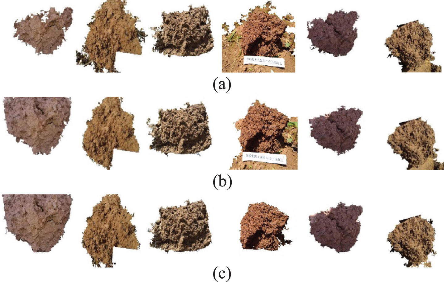
15 robust sample groups are composed of 45 robust images that are artificially selected and there are the characteristics of big shadow in the purple soil area and structure damage purple soil in the background. The images of No. 6 Group are shown in Figure 6.

Fig. 6

Images of Robust No. 6 Group.

5.2 Segmentation validity function

Eq. (28) is the mathematical function of Jaccard index [23], which is used to evaluate the segmentation performance of related algorithms in this paper. The larger the Jaccard index is, the better the segmentation accuracy (SA) is.

$SA (A_{1}, A_{2}) = | A_{1} \cap A_{2} | / | A_{1} \cup A_{2} | \times 100 %$ (32) Where A₂ is the number of pixels belonging to the purple soil found by algorithms, and A₁ denotes the number of pixels belonging to purple soil in the Ground Truth.

5.3 Evaluating the effectiveness of initializing the clustering centers

To test the effectiveness of initializing the clustering centers, the segmenting accuracy of SWFCM with different clustering numbers is tested on normal images (No. 4 Group) and robust images (No. 6 Group). Table 2 gives the clustering centers obtained by our proposed algorithm, and Figure 7 shows the segmentation accuracy of SWFCM under different clustering numbers. In Table 2 and Figure 7, SWFCM provides better segmentation accuracy for Normal No. 4 Group and the Robust No. 6 Group when the clustering centers are obtained by our proposed algorithm. This reflects that our proposed algorithm is effective for the initialization of the clustering center.

Table 2
The clustering centers obtained by our proposed algorithm

Images The clustering centers

Normal No. 4 Group(a) 0.124,6.203

Normal No. 4 Group(b) -0.390,4.558

Normal No. 4 Group(c) -0.819,3.153

Robust No. 6 Group(a) -0.044,4.949,7.992

Robust No. 6 Group(b) -6.257,-0.282,9.675

Robust No. 6 Group(c) -1.646,0.236,3.351

Images	The clustering centers
Normal No. 4 Group(a)	0.124,6.203
Normal No. 4 Group(b)	-0.390,4.558
Normal No. 4 Group(c)	-0.819,3.153
Robust No. 6 Group(a)	-0.044,4.949,7.992
Robust No. 6 Group(b)	-6.257,-0.282,9.675
Robust No. 6 Group(c)	-1.646,0.236,3.351

Fig. 7

Segmentation accuracy using SWFCM with Normal No. 4 Group and Robust No. 6 Group.

5.4 Segmentation results and analysis of different FCM algorithms

To test and verify advantage of SWFCM on segmentation accuracy, five improved FCM algorithms, such as EnFCM, FGFCM, NWFCM, FRFCM and SWFCM, are used to test segmenting accuracy for Normal No. 4 Group and the Robust No. 6 Group. Figure 8 shows the image results of five improved FCM algorithms, and their post-processing results are shown in Figure 9. Table 3 and Table 4 give the segmentation accuracy and execution time of the image results in Figure 8 and Figure 9.

Table 3
The evaluation index of the image results given in Figure 8

Algorithms Index Normal No. 4 Group Robust No. 6 Group

(a) (b) (c) Mean (a) (b) (c) Mean

EnFCM SA% 89.07 68.02 63.68 73.59 63.36 75.44 67.94 68.91

TIME/s 1.216 1.418 1.626 1.420 1.170 1.158 1.862 1.397

FGFCM SA% 89.77 69.98 60.86 73.54 46.61 75.75 65.94 62.77

TIME/s 1.599 1.793 1.915 1.769 1.236 1.517 2.21 1.654

NWFCM SA% 91.61 71.93 54.12 72.55 65.11 80.61 70.64 72.12

TIME/s 6.872 7.643 10.15 8.220 6.402 7.032 8.671 7.368

FRFCM SA% 86.65 67.03 65.63 73.10 36.35 72.08 66.22 58.22

TIME/s 1.864 2.421 2.181 2.155 2.209 1.681 2.559 2.150

SWFCM SA% 89.61 73.08 74.04 78.91 71.63 76.58 68.24 72.15

TIME/s 1.991 1.441 1.970 1.801 2.573 1.254 2.903 2.243

Algorithms	Index	Normal No. 4 Group	Robust No. 6 Group
EnFCM	SA%	89.07	68.02	63.68	73.59	63.36	75.44	67.94	68.91
	TIME/s	1.216	1.418	1.626	1.420	1.170	1.158	1.862	1.397
FGFCM	SA%	89.77	69.98	60.86	73.54	46.61	75.75	65.94	62.77
	TIME/s	1.599	1.793	1.915	1.769	1.236	1.517	2.21	1.654
NWFCM	SA%	91.61	71.93	54.12	72.55	65.11	80.61	70.64	72.12
	TIME/s	6.872	7.643	10.15	8.220	6.402	7.032	8.671	7.368
FRFCM	SA%	86.65	67.03	65.63	73.10	36.35	72.08	66.22	58.22
	TIME/s	1.864	2.421	2.181	2.155	2.209	1.681	2.559	2.150
SWFCM	SA%	89.61	73.08	74.04	78.91	71.63	76.58	68.24	72.15
	TIME/s	1.991	1.441	1.970	1.801	2.573	1.254	2.903	2.243

Table 4

The evaluation index of the image results given in Figure 9 after post-processing

Algorithms	Index	Normal No. 4 Group				Robust No. 6 Group
		(a)	(b)	(c)	Mean	(a)	(b)	(c)	Mean
EnFCM	SA%	95.71	86.33	70.95	84.33	80.05	91.89	85.49	85.81
	TIME/s	0.393	0.535	0.683	0.537	0.229	0.288	0.486	0.334
FGFCM	SA%	95.89	89.24	64.64	83.26	31.88	92.13	80.17	68.06
	TIME/s	0.418	0.512	0.746	0.559	0.024	0.305	0.459	0.263
NWFCM	SA%	95.78	87.54	54.01	79.11	81.71	92.01	81.17	84.96
	TIME/s	0.419	0.682	0.683	0.595	0.213	0.318	0.483	0.338
FRFCM	SA%	95.79	87.34	75.41	86.18	14.08	92.10	87.43	64.54
	TIME/s	0.438	0.565	0.899	0.634	0.018	0.560	0.458	0.345
SWFCM	SA%	96.37	90.22	91.06	92.55	89.60	92.94	86.51	89.68
	TIME/s	0.162	0.159	0.146	0.156	0.101	0.109	0.119	0.110

In the experiment, all FCM algorithms use the ’a’ color component to cluster. A fixed 3 × 3 window is used to filter in the FCM algorithm involving filtering for fair comparison. Common parameters of all FCM algorithms are ψ = 1,m = 2,δ = 0.5,T = 100. In addition, α is used to control the effect of the neighbor term in EnFCM and NWFCM, experientially, α = 1. In FGFCM, the spatial scale factor and the gray-level scale factor are λ_s = 3 and λ_g = 0.5, respectively.

Figure 8 shows SWFCM obtains a better visual effect than other FCM algorithms. Such as Normal No. 4 Group (c), SWFCM is able to remove the surface soil and white labels, which indicates that it can help the classification of the points at the junction of two clusters. In addition, as can be seen from the image results of Robust No. 6 Group (b) that it is not sensitive to shadow. The possible reason is that the selected color feature is not affected by the shadow. In Table 3, compared with EnFCM, FGFCM, NWFCM and FRFCM, the average segmentation accuracy of normal experimental samples with SWFCM is improved by 5.32%, 5.37%, 6.36% and 5.81% respectively, and the average segmentation accuracy of robust experimental samples is improved by 3.24%, 9.38%, 0.03% and 13.93% respectively. Compared with EnFCM and FGFCM, the average executing time of SWFCM is larger. The reason is that both EnFCM and FGFCM are based on gray level for clustering, while SWFCM is based on pixels. Obviously, the gray level of an image is much smaller than the number of pixels. The average executing time of SWFCM algorithm is less than that of NWFCM and FRFCM. Although FRFCM is based on gray level for clustering, its pre-processing costs are large. While SWFCM has no pre-processing. It can be seen in Figure 9 that the image results are closer to the Ground Truth after post-processing. Table 4 shows that the segmentation accuracy of the image in Figure 9 has greatly increased after post-processing algorithms. This reflects that the post-processing algorithms in this paper are able to remove holes and scattered impurities. In addition, its execution time is fast.

Fig. 8

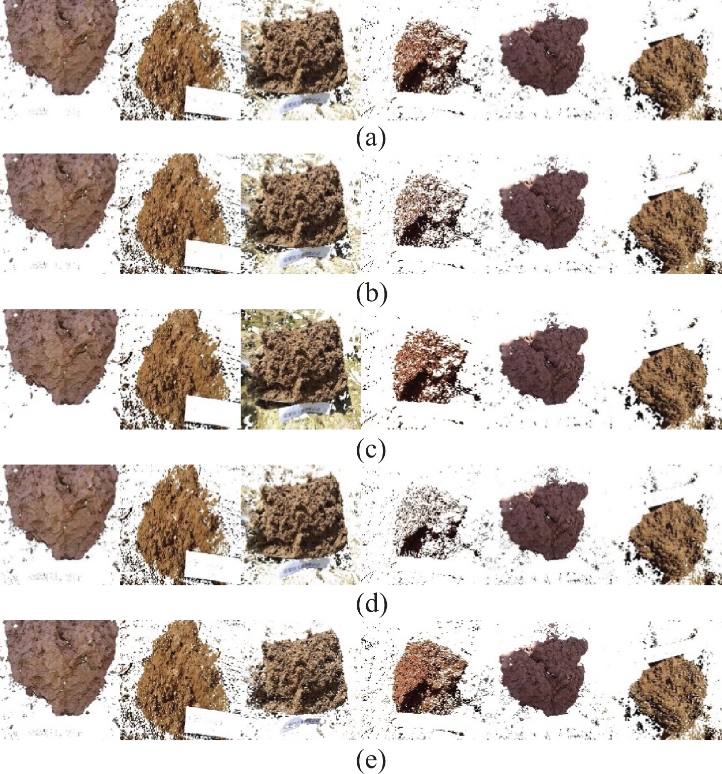
Segmentation results of Normal No. 4 Group and the Robust No. 6 Group using the five FCM algorithms. (a)EnFCM. (b)FGFCM. (c)NWFCM. (d)FRFCM. (e)SWFCM.

Fig. 9

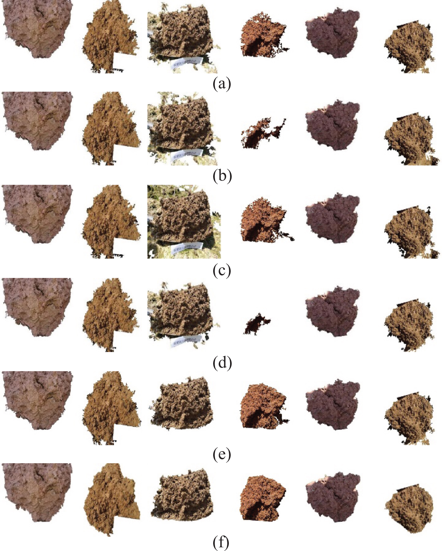
The post-processing results of the image given in Figure 8. (a) EnFCM. (b) FGFCM. (c)NWFCM. (d) FRFCM. (e) SWFCM. (f) Ground truth.

5.5 Segmentation results and analysis of different algorithms

To verify the effectiveness of SWFCM for the segmentation of purple soil color image, 15 groups of normal image examples and 15 groups of robust image examples are used to test segmenting accuracy and execution time with different algorithms which are SWFCM, threshold segmentation algorithm [1] and Improved SLIC algorithm [2]. Figure 10 shows the image results of three algorithms. Table 5 gives the segmentation accuracy and execution time of the image results in Figure 10. Table 6 gives the segmenting accuracy and executing time of 15 groups of normal image examples and 15 groups of robust image examples.

Fig. 10

Segmentation results of Normal No. 4 Group and the Robust No. 6 Group using the relative algorithms. (a) threshold segmentation algorithm (TS). (b) Improved SLIC algorithm(ISLIC). (c) SWFCM.

Figure 10 shows that the segmentation result of the purple soil image with threshold segmentation algorithm is incomplete. Such as Normal No. 4 Group (a), threshold segmentation algorithm divides part of the soil into the background. The reason may be that the fitting effect of normal distribution on h-component histogram of soil is not ideal. In addition, as can be seen from the image results of Robust No. 6 Group (c) that threshold segmentation algorithm failed to correctly classify the topsoil that was similar in color to the purple soil but whose structure had been damaged. Again, improved SLIC algorithm has the same problem. Compared with the improved SLIC algorithm, SWFCM is more accurate for the segmentation of the detailed information of the purple soil boundary.

Table 5 shows that compared with threshold segmentation algorithm and improved SLIC algorithm, the average segmentation accuracy of robust experimental samples with SWFCM is improved by 16.57% and 19.37% respectively.

Table 5

The evaluation index of the image given in Figure 10

Algorithms	Index	Normal No. 4 Group				Robust No. 6 Group
		(a)	(b)	(c)	Mean	(a)	(b)	(c)	Mean
TS	SA%	65.81	80.19	88.33	78.11	55.44	85.33	78.57	73.11
	TIME/s	0.132	0.119	0.139	0.130	0.150	0.121	0.145	0.139
ISLIC	SA%	94.80	93.28	90.06	92.71	42.57	88.09	80.28	70.31
	TIME/s	11.33	14.30	16.77	14.13	7.109	5.710	13.70	8.840
SWFCM	SA%	96.37	90.22	91.06	92.55	89.60	92.94	86.51	89.68
	TIME/s	2.153	1.600	2.116	1.956	2.674	1.363	3.022	2.353

In terms of time cost, threshold segmentation algorithm only uses one threshold to realize image segmentation, which costs less time. Compared with improved SLIC algorithm, SWFCM takes less time to execute, because improved SLIC algorithm spends more time on super-pixel merging. These are also validated by the experimental results of all image sample groups in the Table 6.

Table 6

The evaluation index of 15 groups of normal image examples and 15 groups of robust image examples

Groups	Index	Threshold segmentation algorithm		Improved SLIC algorithm		SWFCM
		Normal	Robust	Normal	Robust	Normal	Robust
1	SA%	86.15±5.22	80.98±8.67	90.58±2.45	84.15±6.38	91.11±0.92	89.06±3.44
	TIME/s	0.125±0.01	0.131±0.01	7.278±6.14	6.094±3.11	1.754±0.25	1.319±0.06
2	SA%	84.78±4.17	78.73±7.81	90.96±2.01	81.54±5.50	91.74±1.95	86.91±0.79
	TIME/s	0.130±0.01	0.139±0.01	10.09±4.96	9.357±4.50	1.644±0.38	1.899±1.04
3	SA%	84.35±3.65	80.44±5.48	92.58±2.64	81.66±5.34	93.51±3.10	87.29±1.44
	TIME/s	0.128±0.01	0.145±0.01	9.522±5.89	8.805±5.37	1.352±0.23	2.432±0.95
4	SA%	78.11±11.4	84.09±7.03	92.71±2.42	81.72±5.79	92.55±3.34	90.49±5.02
	TIME/s	0.130±0.01	0.141±0.01	14.13±2.73	7.440±5.43	1.956±0.31	1.965±0.79
5	SA%	88.02±2.07	80.14±13.8	89.37±0.75	81.75±17.9	92.35±1.46	82.38±16.1
	TIME/s	0.129±0.01	0.130±0.01	6.286±4.45	6.677±3.51	1.646±0.38	1.884±0.65
6	SA%	87.59±2.12	77.13±15.7	91.00±3.34	70.31±24.3	93.07±3.10	89.68±3.21
	TIME/s	0.127±0.01	0.139±0.02	5.723±4.85	8.840±4.27	1.429±0.23	2.353±0.87
7	SA%	89.31±2.03	80.02±4.76	91.29±3.20	81.84±5.63	93.68±2.34	89.47±3.25
	TIME/s	0.135±0.02	0.141±0.02	2.625±0.51	6.888±5.91	1.431±0.24	2.436±0.94
8	SA%	87.06±1.26	83.66±6.83	91.47±2.89	87.11±9.51	93.79±2.66	92.66±3.57
	TIME/s	0.135±0.01	0.136±0.02	6.296±4.44	4.844±2.39	1.496±0.47	1.969±0.79
9	SA%	88.78±1.99	79.72±13.5	91.76±2.65	81.92±18.1	93.35±2.73	84.56±17.3
	TIME/s	0.143±0.01	0.125±0.01	3.198±1.32	4.760±2.49	1.572±0.44	1.888±0.65
10	SA%	87.94±2.69	75.24±3.87	91.68±2.74	78.07±1.92	94.31±1.90	87.76±1.23
	TIME/s	0.140±0.01	0.146±0.01	2.521±0.46	7.159±5.72	1.321±0.18	2.402±1.00
11	SA%	87.36±6.29	78.89±9.55	92.13±3.19	83.34±11.1	90.25±1.79	90.96±4.48
	TIME/s	0.119±0.002	0.142±0.01	10.33±6.43	5.115±2.28	1.708±0.17	1.855±0.69
12	SA%	90.07±1.82	74.94±10.1	91.01±3.17	78.16±17.3	90.53±1.85	82.85±16.3
	TIME/s	0.126±0.01	0.131±0.01	7.102±5.84	5.031±2.39	1.852±0.22	2.402±1.00
13	SA%	88.70±3.09	81.41±7.12	91.39±2.76	84.51±10.2	91.16±2.73	90.52±4.98
	TIME/s	0.131±0.01	0.144±0.01	9.908±4.74	8.107±5.34	1.742±0.40	2.549±0.75
14	SA%	88.27±3.25	77.46±11.6	93.02±2.90	79.32±17.3	92.93±4.04	85.42±10.1
	TIME/s	0.129±0.01	0.133±0.01	9.346±5.68	8.023±5.46	1.450±0.40	2.468±0.71
15	SA%	89.99±2.60	76.66±12.6	93.31±2.39	78.28±17.3	92.49±3.95	83.23±8.48
	TIME/s	0.137±0.09	0.137±0.02	6.248±6.53	4.479±2.67	1.527±0.37	2.388±0.61
Mean	SA%	87.10±3.58	79.30±9.23	91.62±2.63	80.91±11.6	92.46±2.52	87.55±6.65
	TIME/s	0.131±0.02	0.137±0.01	7.374±4.33	6.775±4.06	1.592±0.31	2.147±0.77

6 Conclusion

In this paper, An adaptive scale weighted fuzzy c-means clustering for the segmentation of purple soil color image has been proposed to improve the segmentation quality. The following conclusions are drawn.

(1) The maximum difference optimization model is established with the mean of the Gaussian distance to optimize the parameter ɛ. Then, this parameter ɛ is used to adaptively initialize the clustering centers of FCM algorithm. The experimental results show that this model is helpful to initializing the clustering centers.

(2) The objective function of FCM is reconstructed by weighting the Euclidean distance between the pixel and the clustering center with the compactness of each cluster. Experimental results show that the SWFCM algorithm is effective in improving the segmentation accuracy of purple soil images.

(3) Aiming at the problem of removing scattered impurities and filling holes, the algorithm of extracting the boundary of the purple soil region and the algorithm of filling the purple soil region are proposed. The experimental results show that the post-processing algorithms are effective and their executing time is fast.

Although the effectiveness of the proposed algorithms is promising, some open issues remain to be resolved in the future. Firstly, there is much room for improving the segmentation accuracy of robust images. Secondly, it is necessary to reduce the time cost of SWFCM algorithm so that it can be applied to high-resolution soil images.

Footnotes

Acknowledgments

This work supported by the Key Science and Technology Research Program (No.KJZD-K201900505) and Chongqing University Innovation Research Group funding (No.CXQT20015) of Chongqing Municipal Education Commission, China.

References

Cheng

, Zeng

, Luo

, et al., The color image segmentation of purple soil with its H threshold, Journal of Chongqing Normal University (Natural Science) 36 (2019), 86–95.

, Zeng

, et al., Color image segmentation of purple soil based on improved SLIC, Journal of Chongqing Normal University (Natural Science) 36 (2019), 106–116.

Zeng

, Luo

, Yang

, et al., Color image segmentation of purple soil based on chebyshev inequality, Journal of Southwest University (Natural Science Edition) 41 (2019), 141–150.

Windham

M.P.

, Cluster validity for the fuzzy c-means clustering algorithm, IEEE Transactions on Pattern Analysis and Machine Intelligence 4 (1982), 357–363.

Ruspini

E.H.

, A new approach to clustering, Information and Control 15 (1969), 22–32.

Guo

F.F.

, Wang

X.X.

and Shen

, Adaptive fuzzy c-means algorithm based on local noise detecting for image segmentation, IET Image Processing 10 (2016), 272–279.

Rajaby

, Ahadi

S.M.

and Aghaeinia

, Robust color image segmentation using fuzzy c-means with weighted hue and intensity, Digital Signal Processing 51 (2016), 170–183.

Zheng

, Zhang

, Huang

, et al., Adaptive image segmentation method based on the fuzzy c-means with spatial information, IET Image Processing 12 (2018), 785–792.

Bai

, Li

and Fu

, A fuzzy clustering segmentation method based on neighborhood grayscale information for defining cucumber leaf spot disease images, Computers and Electronics in Agriculture 136 (2017), 157–165.

10.

Namburu

, Samayamantula

S.K.

and Edara

S.R.

, Generalised rough intuitionistic fuzzy c-mean for magnetic resonance brain image segmentation, IET Image Processing 11 (2017), 777–785.

11.

Halder

and Guha

, Medical image segmentation using roughspatial kernelized FCM algorithm, in: Proceedings of International Conference on Advances in Computing, Communications and Informatics (ICACCI), IEEE, Udupi, (2017), 818–823.

12.

Liu

, Zhao

and Zhang

, Image fuzzy clustering based on the region-level markov random field model, IEEE Geoscience and Remote Sensing Letters 12 (2015), 1770–1774.

13.

, Jiao

and Yang

, A multi-kernel joint sparse graph for SAR image segmentation, IEEE Journal of Selected Topics in Applied Earth Observations and Remote Sensing 9 (2016), 1265–1285.

14.

Ahmed

M.N.

, Yamany

S.M.

and Mohamed

, A modified fuzzy c-means algorithm for bias field estimation and segmentation of MRI data, IEEE Transactions on Medical Imaging 21 (2002), 193–199.

15.

Chen

and Zhang

, Robust image segmentation using FCM with spatial constraints based on new kernel-induced distance measure, IEEE Transactions on Systems, Man, and Cybernetics, Part B(Cybernetics) 4 (2004), 1907–1916.

16.

Szilagyi

, Benyo

and Szilagyi

S.M.

, MR brain image segmentation using an enhanced fuzzy c-means algorithm, in: Proceedings of the 25th Annual International Conference of the IEEE Engineering in Medicine and Biology Society, IEEE, Cancun, (2003), 724–726.

17.

Cai

, Chen

and Zhang

, Fast and robust fuzzy c-means clustering algorithms incorporating local information for image segmentation, Pattern Recognition 40 (2007), 825–838.

18.

Zhao

, Cheng

and Cheng

, Neighbourhood weighted fuzzy c-means clustering algorithm for image segmentation, IET Image Processing 8 (2014), 150–161.

19.

Lei

, Jia

and Zhang

, Significantly fast and robust fuzzy cmeans clustering algorithm based on morphological reconstruction and membership filtering, IEEE Transactions on Fuzzy Systems 26 (2018), 3027–3041.

20.

and Ma

, A kernel fuzzy clustering infrared image segmentation algorithm based on histogram and spatial restraint, in: Proceedings of the 9th International Congress on Image and Signal Processing, Bio-Medical Engineering and Informatics (CISPBMEI), Datong, (2016), 313–318.

21.

Luenberger

D.G.

, Optimization by vector space methods, Students Quarterly Journal 41 (1969), 207.

22.

Wang

, et al., DB50T796-2017 Classfication and codes for Chongqing soil, Issued by Chongqing Bureau of Technical Supervision, (2017). (in Chinese)

23.

Jaccard

, The distribution of the flora in the alpine zone, New Phytologist 11 (1912), 37–50.