Research on aesthetic models based on neural architecture search

Abstract

Computational aesthetics, which uses computers to learn human aesthetic habits and ultimately replace humans in scoring images, has become a hot topic in recent years due to its wide application. Most of the initial research is to manually extract features and use classifiers such as support vector machines to score images. With the development of deep learning, traditional manual feature extraction methods are gradually replaced by convolutional neural networks to extract more comprehensive features. However, it is a huge challenge to artificially design an aesthetic neural network. Recently, Neural Architecture Search has upsurged to find suitable neural networks for many tasks in deep learning. In this paper, we first attempt to combine Neural Architecture Search with computational aesthetics. We design and apply a customized progressive differentiable architecture search strategy to obtain a light-weighted and efficient aesthetic baseline model. In addition, we simulate the multi-person rating mechanism by outputting the distribution of the aesthetic value of the image, replacing the previous classification scheme of judging the beauty and unbeauty of the image by the threshold value, and propose a self-weighted Earth Mover’s Distance loss to better fit human subjective scoring. Based on the baseline model, we further introduce several strategies including an attention mechanism, the dilated convolution, and adaptive pooling, to enhance the performance. Finally, we design several groups of comparative experiments to demonstrate the effectiveness of our baseline aesthetic model and the introduced improvement strategies.

Keywords

Artificial intelligence deep learning convolutional neural networks computational aesthetics neural architecture search

1 Introduction

Aesthetic perception refers to the intuitive feeling of human beings on an image they see. Although aesthetics perception is a subjective attribute, to a certain extent, people agree that certain images are indeed more attractive than others, which also derives a current emerging field, computational aesthetics. The purpose of the study of computational image aesthetics is to simulate the human visual system and aesthetic thinking to judge the aesthetic value of images.

The implementation process of computational aesthetics consists of aesthetic feature extraction and aesthetic decision-making. Aesthetic feature extraction can be divided into traditional methods and deep learning methods, among which the traditional methods include extracting features manually and using local image descriptors. Aesthetic decision-making is essential to use the extracted aesthetic features to train a classification or regression model to complete the computational aesthetics task.

Deep Convolutional Neural Network (CNN) has been widely used in computational aesthetics and has achieved promising results. Ma et al. [1] present an Adaptive Layout-Aware Multi-Patch Convolutional Neural Network (A-Lamp CNN) architecture that can accept images of any size while learning from fine-grained details and overall image layout. Wang et al. [2] propose a visual perception network (VP-Net) which is designed as a double-subnet network and can learn from subject region feature and multi-level features. Chen et al. [3] develop an adaptive fractional dilated convolution (AFDC) module which is composition-preserving and parameter-free to enhance the robustness of the model. Shu et al. [4] propose a novel Deep Convolutional Neural Network with Privileged Information (PI-DCNN) which utilizes prior knowledge of photos and photographic elements as privileged information. Zhang et al. [5] present Multimodal Self-and-Collaborative Attention Network (MSCAN) to encode the global composition of images and correlation of multi-modal features. The proposed MSCAN outperforms the state-of-the-art by a large margin for unified aesthetic prediction tasks.

Although these well-designed network structures have achieved excellent results in computational aesthetics tasks, it is extremely challenging to design an aesthetic feature extraction network from scratch and requires repeated verification of the effectiveness of the design. Therefore, most studies use existing classification models as the backbone to extract features and add other branches to these models to improve the feature extraction capabilities of the model. However, these classification models have a large number of parameters. For example, using the VGG network as the backbone, the model parameters reach hundreds of megabytes, which is not suitable for platforms such as mobile terminals.

In this paper, we explore the combination of Neural Architecture Search (NAS) [6] and computational aesthetics. Through the customized search strategy, a powerful feature extraction network suitable for aesthetic tasks can be obtained, and the difficulties and repeated verification problems in the process of designing aesthetic networks can be solved. Compared with conventional convolutional neural networks that only use ordinary convolution operations, we introduce dilated convolution [7] and depthwise separable convolution [8] to expand the receptive field of convolution and reduce the number of convolution parameters to enhance the ability of feature extraction and generalization of the model. In addition, we analyze the commonly used aesthetic assessment dataset and find that the distribution of aesthetic scores obtained by human subjective ratings is close to the normal distribution. Therefore, we propose a self-weighted Earth Mover’s Distance loss to better fit human aesthetic habits. After searching for the baseline model, we make a series of improvements to the model, including the introduction of adaptive pooling to ensure the integrity of the picture, and the use of an attention mechanism [9] to assign different weights to different regions of the picture to further improve the performance of the baseline model. The contributions of this paper can be summarized as follows:

To the best of our knowledge, this paper is the first exploration of applying NAS to computational aesthetics. Through customized end-to-end search, a light-weighted and powerful baseline model suitable for aesthetic tasks can be obtained. We named it AestheticNet, which can achieve promising results on the current public aesthetic datasets.

By analyzing the distribution of human opinion scores, we propose a self-weighted Earth Mover’s Distance (EMD) loss, so that our model can better fit the distribution of human scoring.

We use dilated convolution and depthwise separable convolution to replace ordinary convolution operations and introduce adaptive pooling and attention mechanisms to further improve the performance of the AestheticNet.

Compared with other research works, our model is simpler, lighter, and easy to be deployed on resource-constrained devices, thus having better application value. In addition, the network we search can be used as the backbone network for other research works, which we believe can bring certain performance improvements.

2 Related work

2.1 Computational aesthetics

The common tasks of computational aesthetics include image quality evaluation and image aesthetic evaluation and there is abundant literature on these two tasks. These efforts can be broadly divided into those based on hand-crafted features and those based on deep learning methods. The method of hand-crafted features is assumed to model the empirical photographic rules and certain objective aspects of the image. For example, Datta et al. [10] extract 56-dimensional features from each image, including exposure of light, colorfulness, saturation, rule of thirds, etc. Tang et al. [11] focus on aesthetic assessment of image content. Photos are divided into seven categories, and visual features are extracted in different ways according to the diversity of photo content. Guo et al. [12] propose to combine manual features and semantic features for image aesthetic assessment. Chamaret et al. [13] focus on color information and develop a harmony-guided image aesthetic quality assessment method.

Recently, deep learning methods have shown great advantages over hand-crafted features in learning rich features. Talebi et al. [14] introduce a CNN-based image assessment method, NIMA, which can be trained on aesthetics and pixel-level quality datasets. Li et al. [15] propose an end-to-end personality-driven multi-task deep learning model for general image aesthetic assessment. Pan et al. [16] propose an adversarial learning framework that uses aesthetic attributes as privileged information to build better predictors. Li et al. [17] propose a personality-assisted multi-task deep learning framework for general and personalized image aesthetics assessment. Takimoto et al. [18] propose an aesthetic assessment method based on multi-stream and multi-task convolutional neural networks (CNNs) to extract global features and salient features from input images. Although these methods have made great progress, most of them use classification models as feature extraction networks and add some additional branches to assist training. The models are complex and have a large amount of parameters, which are not conducive to deployment.

2.2 Network architecture search

In recent years, the development of Neural structure search (NAS) has changed the traditional way of model design from manual to automatic and has achieved remarkable success in various perceptual tasks including image classification, object detection, and semantic segmentation. The overall framework of NAS is shown in Figure 1.

Fig. 1

Flowchart of Neural Architecture Search method. The search strategy selects architecture A from the predefined search space $O$ , passes architecture to the performance estimation strategy, which returns the performance estimation result of A to the search strategy.

The work of NAS-RL [6] is considered a pioneering work of NAS. The idea of NAS-RL is that the architecture of a neural network can be described as a variable-length string. Therefore, NAS-RL uses Recurrent Neural Network (RNN) as a controller to generate such a string and then uses Reinforcement Learning (RL) to optimize the controller, and finally obtain a satisfactory network structure. NASNet [19] benefits from the idea of artificial network architecture design and proposes a modular search strategy, which is later widely adopted. AmoebaNet [20] aims to use evolutionary algorithms (EA) to automatically learn an optimal network architecture. The tournament selection evolutionary algorithm is modified by introducing an age property to favor the younger genotypes and evolve an image classifier, AmoebaNet-A, whose performance surpasses the artificially designed network for the first time. However, NAS has high requirements for computing. For example, AmoebaNet requires 450 GPUs to search for 7 days on the CIFAR10 dataset to obtain the optimal architecture. To solve this problem, DARTS [21] relaxes the original discrete search space, which makes it possible to optimize the search space of architecture effectively by using gradient and the search can be completed within 4 days on a single GPU. P-DARTS [22] improves DARTS starts with the depth gap between search and evaluation of network architecture and can finish the search within 1 day on a single GPU. The emergence of DARTS makes the engineering practice of NAS possible.

3 Method

3.1 Preliminary

For convolutional neural networks, DARTS searches for a normal cell and a reduction cell and builds the final model by stacking the two types of cell structures. Specifically, a reduction cell is inserted at 1/3 and 2/3 of the model. In the reduction cell, the operation applied to the input has a stride of 2 to reduce the resolution of the input. A cell can be regarded as a directed acyclic graph (DAG) of N nodes ${x_{i}}_{x = 0}^{N - 1}$ , where each node represents a feature map. In DARTS, each cell structure contains 7 nodes, including 2 input nodes, 4 intermediate nodes and 1 output node. We denote the operation space as $O$ , that is, the search space as described in NAS, and each element is a candidate operation, e.g., zero, skip-connect, convolution, pooling, etc. Each edge e^(i,j) of the DAG stands for the information flow from node x_i to x_j and is composed of candidate operations weighted by the architecture parameter α^(i,j). Each edge e^(i,j) can be formulated by a function ${\bar{o}}^{(i, j)}$ , where ${\bar{o}}^{(i, j)} (x_{i}) = \sum_{o \in O} f_{o}^{(i, j)} \cdot o (x_{i})$ , and the weight of each operation $o \in O$ is the softmax of the architecture parameter α^(i,j), specifically $f_{o}^{(i, j)} = \frac{\exp (α_{o}^{(i, j)})}{\sum_{o^{'} \in O} \exp (α_{o^{'}}^{(i, j)})}$ . The intermediate node is $x_{j} = \sum_{i < j} {\bar{o}}^{(i, j)} (x_{i})$ . The output node x_N-1 is depth-wise concatenation of all the intermediate nodes except input nodes. The above hyper-network is called a one-shot model, and the weight of this hyper-network is expressed by ω.

For the search process, we express $L_{train}$ and $L_{val}$ as training loss and validation loss, respectively. Then we can learn the architecture parameters through the following bi-level optimization problem: $\begin{matrix} \min_{α} L_{val} (ω^{*} (α), α) \\ s . t . ω^{*} (α) & = \arg \min_{ω} L_{train} (ω, α) . \end{matrix}$ (1) Once the architecture parameter α is obtained, the final discrete model can be derived in the following way: 1) setting $o^{(i, j)} = \arg \max_{o \in O, o \notin zero} f_{o}^{(i, j)}$ ; 2) for each intermediate node, select two incoming edges with a maximum value of $\max_{o \in O, o \notin zero} f_{o}^{(i, j)}$ .

Restricted by the memory size of the GPU, DARTS must search for a model in the shallow network (consisting of 8 cells) and evaluate it in the deep network (consisting of 20 cells). However, there are big differences in the behavior of the shallow and deep networks, which means that the structure we choose in the search process is not necessarily optimal. Chen et al. in the P-DARTS paper name this issue depth gap and demonstrate that it makes normal cells of the discovered models tend to maintain shallow connections rather than deep ones. This is because shallow networks generally enjoy faster gradient descent during the search process, contradicting the common sense that deeper networks tend to perform better. To bridge the depth gap, they adopt a strategy of gradually increasing the network depth during the search process, so that at the end of the search, the depth is close enough to the setting used in the evaluation. P-DARTS achieved the fastest NAS speeds at that time, achieving an error rate of less than 3% on the CIFAR10. The difference between DARTS and P-DARTS is shown in Figure 2.

Fig. 2

Difference between DARTS and P-DARTS. Green and blue indicate search and evaluation, respectively.

3.2 Self-weighted loss function

In this paper, our goal is to predict the rating distribution of a given image. The actual distribution of human ratings for pictures can be expressed as the empirical probability quality function p = [p_{s
₁}, . . . , p_{s
_N}],, s₁ ⩽ s_i ≤ s_N, where s_i represents the i-th score bucket and N represents the total number of score buckets. Aesthetic rating distribution prediction can be regarded as an ordered-class classification task, so loss functions such as MSE and cross-entropy without considering inter-class relations are not the best choice for this problem. Also known as the Wasserstein distance, Earth Mover’s Distance (EMD) is the minimum cost of converting one distribution to another. EMD loss is applied to classification tasks with predefined inter-class similarity metrics and has been widely used as a learning objective for aesthetic score distribution prediction tasks. The formula for EMD loss is as follows: $L (p, \hat{p}) = \frac{1}{N} \sum_{k = 1}^{N} {| {CDF}_{p}^{(k)} - {CDF}_{\hat{p}}^{(k)} |}^{r}$ (2) Where ${CDF}_{p}^{(k)}$ represents the k-th cumulative density function (CDF) of the ground-truth distribution p and ${CDF}_{\hat{p}}^{(k)}$ represents the k-th CDF of the predicted distribution $\hat{p}$ . r stands for the power of r, generally choose 1 or 2.

The AVA dataset [23] is a commonly used dataset for aesthetic assessment, and each image in the dataset has a discrete score ranging from 1 to 10 voted by 78 to 549 people. The average score of an image is often considered to be its ground truth label. The distribution of aesthetic scores on the AVA dataset is shown in Figure 3.

Fig. 3

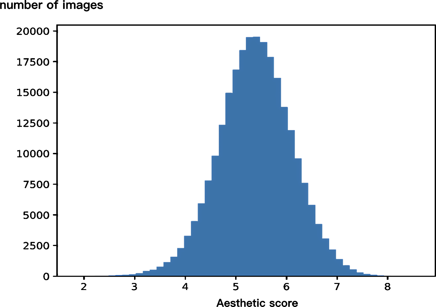
The distribution of aesthetic scores on the AVA dataset.

Through observation, we find that the data distribution of the AVA aesthetic dataset is approximately normal distribution, in which most of the scores are clustered around 4, 5, and 6, which is in line with our daily aesthetic habits and human scoring habits. Therefore, we believe that the ground truth rating distribution of each picture, p itself, can actually be used as a weight term, which can be incorporated into the calculation of loss function to better fit the distribution of human subjective ratings. The self-weighted EMD loss we proposed is illustrated as follows: $\hat{L} (p, \hat{p}) = \frac{1}{N} \sum_{k = 1}^{N} {| ({CDF}_{p}^{(k)} - {CDF}_{\hat{p}}^{(k)}) * p |}^{r}$ (3)

3.3 Aesthetic model search

Thanks to the efficient search speed of P-DARTS and the ability to search for specific network structures, we customize P-DARTS so that the network structure suitable for aesthetic tasks can be obtained through search. We aim to search for a light-weighted and powerful aesthetic model that is small enough to be easily deployed on micro terminals. The entire search process and training process are shown in Figure 4.

Fig. 4

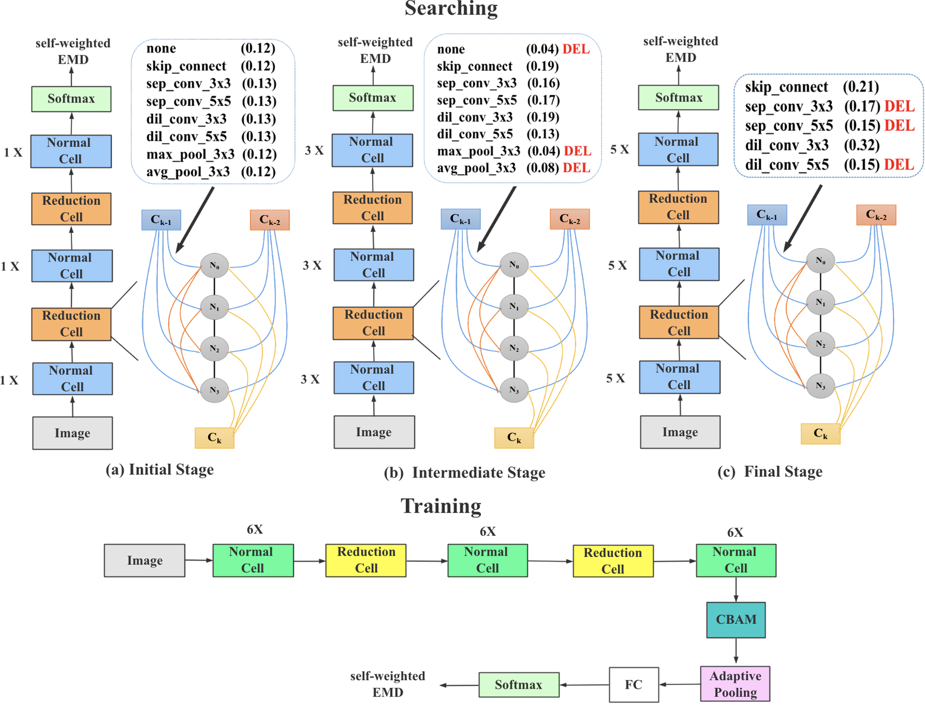
The overall pipeline of our customized search and training. For simplicity, only reduction cells are displayed. The depth of the search network increases from 5 in the initial phase to 11 and 17 in the intermediate and final stages, while the number of candidate operations for each edge decreases from 8 to 5 and 2. The operations with the lowest score in the previous stage of each edge are eliminated (marked with a bold "DEL"). We use the final score to get the optimal normal cells and reduction cells. During the training phase, we use the searched normal cell (marked green) and reduction cell (marked yellow) to train on the target dataset in combination with the introduced improvement strategy.

Currently, the mainstream search strategy is based on modular search strategy, namely, search normal cell and reduction cell, and build the final model by stacking the two types of cell structures. To speed up the search, the search process is typically performed on a relatively small dataset, also known as the proxy dataset, to obtain these two cell structures. The final model is then retrained for validation on other datasets, also known as target datasets. In particular, the target dataset can also be the proxy dataset itself.

P-DARTS uses DARTS as the backbone framework, and the entire search process consists of three stages. In the initial stage, the search space and network configuration are the same as DARTS, except that the number of cells is set to 5. In the intermediate stage, the number of cells increases from 5 to 11. To balance the GPU memory overhead caused by the increase of network layers, P-DARTS screen the top-5 candidate operations according to the α parameter to continue searching. Similarly, in the last phase, the number of cells increases from 11 to 17, and the candidate operations of top-2 on each edge are retained for searching. P-DARTS stacks 20 cell structures searched from the CIFAR10 dataset and achieves state-of-the-art results on the target datasets CIFAR10 and ImageNet.

In this paper, we make customized modifications to P-DARTS so that the network can search for cell structures suitable for aesthetic tasks. The original P-DARTS search process is aimed at object recognition tasks, and the input is the image containing a single label, and the loss function used is the cross-entropy. In order to make the search process suitable for aesthetic tasks, we replace the original input with a multi-label input that simulates the multi-person scoring prediction distribution, and replace the cross-entropy loss with the self-weighted EMD loss we proposed in the previous section. We search on the generic AVA aesthetic dataset, and since this dataset is relatively large, we take a part of the AVA training set as the proxy dataset for the search.

Different from the traditional artificial convolutional neural network, which only uses ordinary convolution operation, we introduce two kinds of convolution, the dilated convolution and the depthwise separable convolution, into the candidate operation, in order to find a light-weighted network with stronger feature extraction ability. The set of candidate operations for the search space is set as follows: 3×3 depthwise separable convolution (sep_conv_3x3), 5×5 depthwise separable convolution (sep_conv_5x5), 3×3 dilated convolution (dil_conv_3x3), 5×5 dilated convolution (dil_conv_5x5), 3×3 max pooling (max_pool_3x3), 3×3 average pooling (avg_pool_3x3), skip_connect, none. Here skip_connect is similar to the residual connection in ResNet, and None means that there is no operation between the two nodes.

Dilated convolution [7] is widely used in semantic segmentation and object detection tasks because it can expand the receptive field of convolution operations without information loss and without introducing additional parameters. In the aesthetic task, from the perspective of human aesthetics, we can know that the overall view is essential to the aesthetic feeling of images. Therefore, in order to better simulate human aesthetics, the use of a larger receptive field is conducive to improving the performance of the aesthetic model.

Depthwise separable convolution [8] is composed of two modules: depthwise convolution and pointwise convolution, where depthwise convolution performs a convolution operation on each channel of the input feature map, usually 3×3 convolution operation is used, and pointwise convolution uses 1×1 convolution to mix the output of the depthwise convolution. Assume that the convolution kernel size is K, M is the input channel size, and N is the output channel size. Then the parameter quantity required for ordinary convolution is K × K × M × N, and that of depthwise separable convolution is K × K × M + 1 ×1 × M × N. Therefore, the number of parameters of depthwise separable convolution is much less than that of ordinary convolution, thus reducing the computational effort and the risk of overfitting. This is also the reason why the depthwise separable convolution can make the model lighter, accelerate the training speed and improve the performance of the model.

The specific search process is shown in Algorithm 1.

Algorithm 1 Network architecture search for aesthetic models

Input: Training set $D_{train} = {(x^{(i)}, p^{(i)})}_{i = 1}^{N}$ , validation set $D_{val} = {(x^{(i)}, p^{(i)})}_{i = 1}^{M}$ , batch size of the training set n, batch size of the validation set m, number of stages of search k ← 3, number of steps of updating hyper-network K₁, number of training iterations e, learning rate of hyper-network η_t, learning rate of architecture η_v.

Output: normal cell and reduction cell

1: for i = 0 → k do

2: if i = 1 then

3: Generate a hyper-network with 5 cells.

4: end if

5: if i = 2 then

6: Keep the first 5 operations with the largest α value of each edge in the hyper-network.

7: Generate a hyper-network with 11 cells.

8: end if

9: if i = 3 then

10: Keep the first 2 operations with the largest α value of each edge in the hyper-network.

11: Generate a hyper-network with 17 cells.

12: end if

13: Randomly initialize the weight ω of the hyper-network, and the architecture parameter α.

14: for all e do

15: for all K₁ do

16: Sample a mini-batch of n training images ${x^{(i)}}_{i = 1}^{n}$ from $D_{train}$ .

17: Sample a mini-batch of n real labels ${p^{(i)}}_{i = 1}^{n}$ from $D_{train}$ .

18: Sample a mini-batch of m validation images ${x^{(i)}}_{i = 1}^{m}$ from $D_{val}$ .

19: Sample a mini-batch of m real labels ${p^{(i)}}_{i = 1}^{m}$ from $D_{val}$ .

20: Calculate the self-weighted EMD loss $L_{train}$ and $L_{val}$ as Eq. 3.

21: Update the weight ω of super-network by gradient descent $ω : = ω - η_{t} \frac{\partial L_{train} (ω, α)}{\partial ω}$ .

22: Update the architecture parameter α by gradient descent $α : = α - η_{v} \frac{\partial L_{val} (ω, α)}{\partial α}$ .

23: end for

24: end for

25: end for

26: Get the normal cell and reduction cell according to architecture parameter α.

3.4 Attention mechanism

The attention mechanism is a solution proposed by simulating the selective attention mechanism of the human visual system. In short, the attention mechanism is to quickly and purposely screen out valuable information from a large amount of information. The attention mechanism, originally used in the field of natural language processing to encode long sequences of inputs, has now been widely used in various fields of deep learning, such as computer vision and speech.

In this paper, we add the attention mechanism CBAM [9] to the original network to obtain attention weights on the input feature map from the spatial dimension and the channel dimension respectively for weighted output. With the plug-and-play flexibility, CBAM can be divided into two independent modules, channel attention module, and spatial attention module. The channel attention module is responsible for modeling the importance of each channel in the channel dimension, while the spatial attention module models the positional relationship of any two points in the feature map in the spatial dimension. The weight values of the two dimensions tell the convolutional neural network what to pay attention to and which region to pay attention to respectively in the channel and spatial dimensions.

Given a feature map F of size H × W × C, the specific operation of the channel attention mechanism is to perform maximum pooling and average pooling operations channel by channel to obtain two 1 × 1 × C feature maps. Then, these two 1 × 1 × C feature maps are fed into a two-layer weight-sharing neural network (MLP). Subsequently, the MLP output features are subjected to an element-wise addition operation, and the value is controlled to a weight between 0 and 1 through sigmoid activation operation to generate the final channel attention feature, namely M_c. Finally, M_c and the input feature map F are element-wise multiplied. The formula is as follows:

$\begin{matrix} M_{c} & = & σ (MLP (AvgPool (F)) \\ + MLP (MaxPool (F))) \\ = & σ (w_{1} (w_{0} (F_{avg}^{c})) + w_{1} (w_{0} (F_{\max}^{c}))) \end{matrix}$ (4) The input of the spatial attention module is the feature map F of size H × W × C output by the channel attention module. First, perform global max pooling and global average pooling respectively in the channel dimension to obtain two H × W × 1 feature maps. Then, a feature map of H × W × 2 is obtained by the Concat operation of these two feature maps. After that use a 7×7 convolution operation to reduce the dimensionality of the feature map to H × W × 1, and generate spatial attention feature through sigmoid, namely M_s. Finally, the feature is multiplied with the input feature of the module to obtain the final generated feature. The formula is as follows:

$\begin{matrix} M_{s} & = & σ (f^{7 * 7} ([AvgPool (F); MaxPool (F)])) \\ = & σ (f^{7 * 7} ([F_{avg}^{s}; F_{\max}^{s}])) \end{matrix}$ (5)

3.5 Adaptive input

In the fully connected layer, each neuron corresponds to input, that is, the fully connected layer requires a fixed input size. However, the input images are generally of different sizes and have different aspect ratios. If the size of the input image is different, the feature map before the fully connected layer is also different, so the input dimension of the fully connected layer cannot be determined. Therefore, before the image is input into the convolutional neural network, the image is clipped or wrapped to a fixed scale, such as 224×224, 256×256, etc. However, either crop operation or wrap operation destroys the original image structure features to a certain extent. For aesthetic tasks, the integrity of composition features is a very important link in image aesthetics, such as the golden section rule (also known as the rule of thirds), the principle of contrast, the principle of balance and symmetry, etc., which is often heard in photography, reflecting the integrity of composition features. After the crop operation, we can only obtain the information of the cropped part of the picture, and other information is not input to the network, so the subsequent network cannot extract the features of these parts. Similarly, after the warp operation, the picture has actually brought a feeling of visual distortion.

To solve this problem, we insert an adaptive pooling layer between the output of the convolutional layer and the input of the fully connected layer. As the name implies, the adaptive pooling layer is to automatically adjust some parameters of the pooling layer according to the specified output size, so as to achieve the purpose of outputting features of the specified size. The principle of the adaptive pooling layer is as follows. Assuming that the kernel size K, padding P, stride S, and the input size I of the input tensor of the pooling layer are known, then the output size $O$ of the output tensor is: $O = \frac{I + 2 \times P - K}{S} + 1$ (6) According to the above formula, the kernel size can be $K = (I + 2 \times P) - (O - 1) \times S$ (7) In the experiment, we set padding to be 0 and the calculation of the stride is set as follows:

$S = floor (I / O)$ (8)

4 Experiment

4.1 Dataset

At present, the aesthetic model dataset is mainly divided into two categories, one is used for image quality assessment, and the other is used for image aesthetic assessment. The image quality assessment dataset includes TID2013 [24], CSIQ, LIVE, WATERLOO, etc. The mainstream datasets for image aesthetics assessment include the Photo.Net dataset (PN), the DPChallenge.com dataset, the Cu-Photo Quality, and the AVA dataset [23]. An introduction to the aesthetic datasets is shown in Table 1. Most of the experiments in this paper are conducted on the AVA dataset, and the final model is verified on the TID2013 dataset.

Table 1
Aesthetic datasets

Dataset Name The Main Purpose Description

CSIQ Image Quality Assessment 30 reference images, 6 distortion types

LIVE Image Quality Assessment 29 reference images, 5 distortion types

WATERLOO Image Quality Assessment 4,744 reference images, 20 distortion types

TID2013 Image Quality Assessment 25 reference images, 24 distortion types

photo.net Image Aesthetic Assessment 20,278 images, score [0,7]

DPChallenge.com Image Aesthetic Assessment 16,509 images, score [0,10]

CUHK Image Aesthetic Assessment 28,410 images, high quality and low quality

AVA Image Aesthetic Assessment 255,300 images, score [0,10]

Dataset Name	The Main Purpose	Description
CSIQ	Image Quality Assessment	30 reference images, 6 distortion types
LIVE	Image Quality Assessment	29 reference images, 5 distortion types
WATERLOO	Image Quality Assessment	4,744 reference images, 20 distortion types
TID2013	Image Quality Assessment	25 reference images, 24 distortion types
photo.net	Image Aesthetic Assessment	20,278 images, score [0,7]
DPChallenge.com	Image Aesthetic Assessment	16,509 images, score [0,10]
CUHK	Image Aesthetic Assessment	28,410 images, high quality and low quality
AVA	Image Aesthetic Assessment	255,300 images, score [0,10]

The AVA dataset contains 255,530 images, each of which is rated by approximately 200 photography enthusiasts. The aesthetic score ranges from 1 to 10. The AVA dataset is divided into two parts: training set (230,000) and test set (20,000).

The TID2013 dataset is a supplement to TID2008 and is designed to evaluate full-reference perceptual image quality. It has 3000 images, drawn from 25 reference (clean) images, with 24 distortions, each of which has 5 levels. This results in 120 distorted images per reference image, including different types of distortions such as compression artifacts, noise, blur, and color artifacts.

4.2 Evaluating indicators

The commonly used evaluation indicators for aesthetic models include Accuracy, LCC, SROCC, EMD, etc. Each of these metrics is described below.

4.2.1 Accuracy

Classification accuracy, where the aesthetic model is defined as a dichotomous problem, beautiful or not beautiful. The following introduces several common terms in the classification model indicators:

True Positives(TP): The sample is actually positive (beautiful), and the model classifies it as a positive sample.

False Positives(FP): The sample is actually negative (not beautiful), but the model classifies it as a positive sample.

True Negatives(TN): The sample is actually negative (not beautiful), and the model classifies it as a negative sample.

False Negatives(FN): The sample is actually positive (beautiful), but the model classifies it as a negative sample.

The calculation formula of Accuracy is as follows:

Accuracy = \frac{TP + TN}{TP + FP + TN + FN}

(9)

4.2.2 LCC

Linear correlation coefficient (LCC), also known as Pearson correlation coefficient (PLCC), is usually used to compare the difference and correlation between the objective value of the model and the subjective value of the observation. The calculation formula of LCC is as follows: $LCC = \frac{\sum_{i = 1}^{N} (y_{i} - \bar{y}) - (\hat{y_{i}} - \hat{\bar{y_{i}}})}{\sqrt{\sum_{i = 1}^{N} (y_{i} - \bar{y_{i}})^{2}} \sqrt{\sum_{i = 1}^{N} (\hat{y_{i}} - \hat{\bar{y_{i}}})^{2}}}$ (10) In the formula, y_i and $\hat{y_{i}}$ represent the real value and predicted value of the i-th image in the dataset, $\bar{y_{i}}$ and $\hat{\bar{y_{i}}}$ , represent the real mean value and predicted mean value of the image, and N is the number of distorted images.

4.2.3 SROCC

In the aesthetic task, Spearman’s Rank Order Correlation Coefficient (SROCC) is used to evaluate the ranking correlation between the predicted aesthetic score and the real aesthetic score. Assume that c_i and ${\hat{c}}_{i}$ represent the ranking of the i-th test image in the actual and predicted aesthetic scores respectively, then the ranking difference between the actual and predicted aesthetic scores can be calculated as $d_{i} = c_{i} - {\hat{c}}_{i}$ , and SROCC is defined as: $SROCC = 1 - \frac{6 \sum_{i = 1}^{N} d_{i}^{2}}{N (N + 1)}$ (11) Where N is the number of test samples. The value range of SROCC is [-1, 1], and the higher the SROCC value, the better the prediction performance.

4.2.4 EMD

Earth Mover’s Distance (EMD) is usually used to evaluate the closeness between the predicted aesthetic distribution and the real aesthetic distribution. The smaller the EMD value, the better the model performance. The calculation formula for EMD is described in Section 3.2.

4.3 NAS and aesthetic tasks

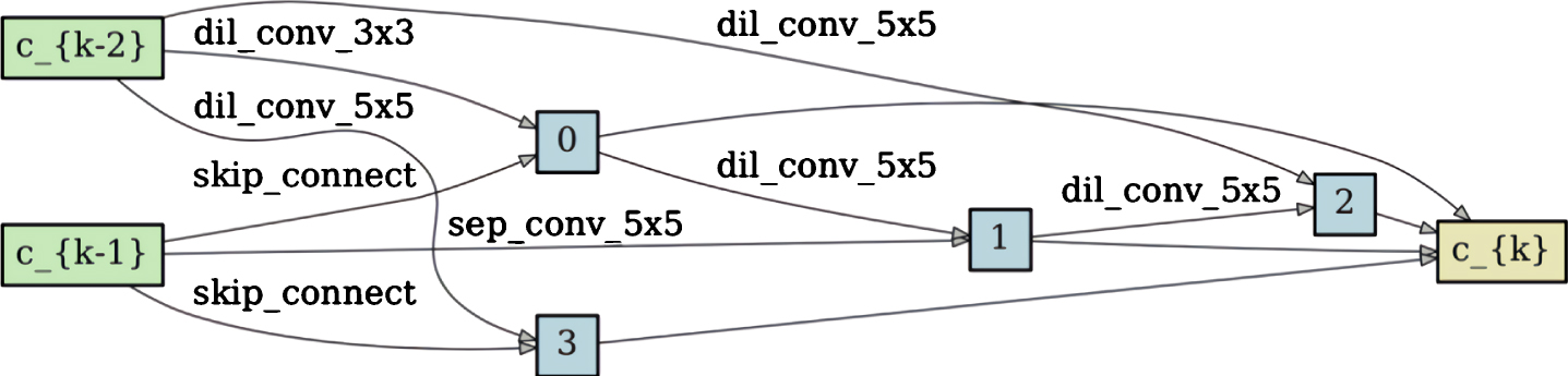
In this section, we use the customized P-DARTS search algorithm to search for normal cell and reduction cell on the AVA dataset. We select 1/10 of the images from the training set, namely about 20,000 images as the proxy dataset, and then divide the proxy dataset into the training set and the validation set at a ratio of 4:1. In the search process, we set the batch size to 96, the initial learning rate to 0.025, randomly initialize the hyper-network parameter ω and the architecture parameter α, the optimizer of the ω is SGD, and the optimizer of the α is Adam. The entire search process consists of three stages. The first stage model is composed of 5 cells, the second stage model is composed of 11 cells, and the third stage model is composed of 17 cells. In each stage, parameters ω and α are updated through iterative bi-level optimization. The number of iterations in each stage is 25, and the optimal parameter α is finally obtained. The normal cell and the reduction cell can be obtained according to parameter α. The normal cell and reduction cell structures obtained by searching on AVA dataset are shown in Figure 5 and Figure 6.

Fig. 5

Normal cell obtained by searching on the AVA dataset.

Fig. 6

Reduction cell obtained by searching on the AVA dataset.

Our baseline model is constructed by stacking 20 searched cells, and we named it AestheticNet. Then, after re-initializing the model parameters randomly, training is performed on the entire training set of the AVA dataset, the initial learning rate is 0.1, and the number of training iterations is 200. After the training is completed, we perform verification on the test set of the AVA dataset. We regard images with aesthetic scores greater than 5 points as high-quality pictures, and those with aesthetic scores less than or equal to 5 points as low-quality pictures, thus transforming the problem of aesthetic assessment into a dichotomy problem. Accuracy is used as an indicator to measure the effect of the aesthetic model. By comparing with some existing studies, the summarized experimental results are shown in Table 2, where the best results are marked in bold font. From the table, we can see that most of the researches uses backbones from image classification tasks, and these networks are generally large in size. In contrast, after using light-weighted convolution operation, the amount of model parameters is greatly reduced, and it is more friendly to miniature terminals. In addition, these backbones are usually pre-trained on the ImageNet dataset or using some auxiliary tasks, and then use the pre-trained weights to initialize the network to fine-tune the aesthetic tasks. However, pre-training requires a lot of time and a lot of annotation data, which is time-consuming and resource-intensive. On the other hand, the current aesthetic model research is based on the backbone, introducing some other branches or adding supervisory information for training to enhance the feature extraction ability of the model. For example, in the table, Sherashiya et al. design the two-channel deep CNN based on the Resnet50 model, which achieves the highest accuracy among all the competitive architectures, but there is almost no work to design backbone for aesthetic tasks. The backbone suitable for aesthetic tasks obtained through a customized search strategy can achieve competitive results without pre-training, which also verifies the effectiveness of our customized search strategy.

Table 2

Accuracy comparison of existing aesthetic assessment methods on AVA dataset

Model Name	Year	Backbone	Params	Pretrained	Accuracy
MTCNN [25]	2017	VGG-16	138,4MB	Y	77.73%
MTRLCNN [25]	2017	VGG-16	138,4MB	Y	78.46%
AA-Net [26]	2017	VGG-16	138,4MB	Y	76.9%
A-Lamp [1]	2017	VGG-16	138,4MB	Y	82.5%
MLAN [27]	2018	Inception-v3	23.8MB	Y	79.38%
AesCNN-W [28]	2018	VGG-16	138,4MB	Y	78.87%
VP-Net [2]	2019	ResNet-50	25.6M	Y	80.55%
GLFN-Net [29]	2019	VGG-16	138,4MB	Y	82.95%
Sheng et al. [30]	2020	ResNet-18	11.7M	Y	82.8%
Sherashiya et al. [31]	2020	Resnet50	25.6M	Y	83.02%
AestheticNet	-	AestheticNet	6.71MB	N	78.3%

4.4 Effect of the self-weighted loss function

Figure 7 and Figure 8 respectively visualize the distribution of prediction results on the test set using the general EMD loss function and the self-weighted EMD loss function. It can be seen from Figure 7 that compared with the actual distribution, the predicted distribution using the conventional EMD loss function is slightly inclined to the right. In contrast, the predicted distribution trained with the self-weighted EMD loss function can better fit the real distribution, as shown in the Figure 8, indicating that when the offset weight is added to the EMD loss function, the predicted distribution is biased to the center of the real distribution, which is more in line with the daily aesthetic habits of human beings.

Fig. 7

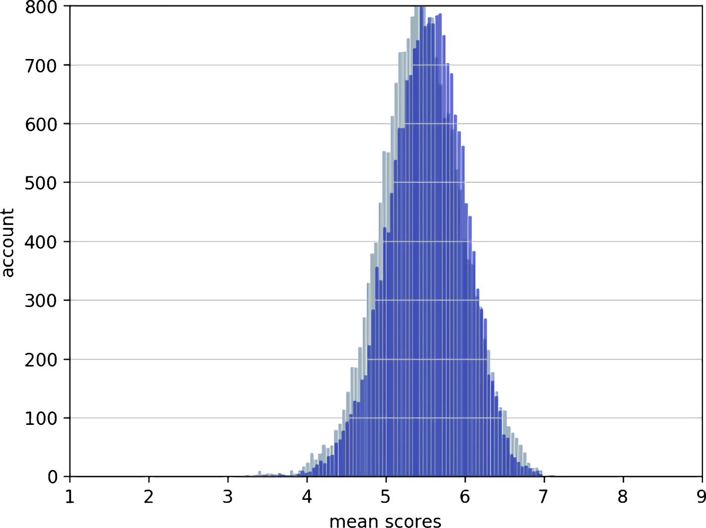
The light color represents the distribution of the actual test set, the dark color represents the distribution predicted by the model, the horizontal axis represents the average score of the image, and the vertical axis represents the number of raters who rate the score.

Fig. 8

The predicted results after trained using self-weighted EMD loss.

To further demonstrate the effectiveness of the self-weighted EMD loss we proposed, we calculate the classification accuracy and EMD value of the two losses respectively according to the dichotomy task and calculate the changes in the mean value and variance of LCC and SROCC, represented by LCC(mean), LCC(var), SROCC(mean) and SROCC(var), which are recorded in Table 3, where the best results are highlighted in bold font. It can also be seen from the experimental data that the model trained with self-weighted EMD loss is indeed better than the model trained with traditional EMD loss, which also verifies the effectiveness of our proposed loss function.

Table 3

Comparisons on the self-weighted loss function

Model Name	LCC(mean)	SROCC(mean)	LCC(var)	SROCC(var)	EMD	Accuracy
AestheticNet	0.623	0.603	0.211	0.214	0.052	78.3%
AestheticNet+self-weighted EMD loss	0.643	0.666	0.213	0.215	0.052	79.6%

4.5 Effect of attention mechanism

We introduce the attention mechanism CBAM on the basis of the baseline model AestheticNet to strengthen the feature extraction ability of the model and then improve the inference performance of the model. Specifically, we add a CBAM module to the tail of the feature extraction network of the model to make the model pay more attention to the important regions of the feature map.

To verify the effectiveness of the introduced attention mechanism CBAM module, we design a model comparison experiment with or without the CBAM module and use the same evaluation index as in the previous section. The results of the comparative experiment of the model are shown in Table 4, and the best results are highlighted in bold font. We can see that the introduction of the CBAM attention mechanism can indeed improve the performance of the model.

Table 4
Comparisons on the attention mechanism

Model Name LCC(mean) SROCC(mean) LCC(var) SROCC(var) EMD Accuracy

AestheticNet 0.623 0.603 0.211 0.214 0.052 78.3%

AestheticNet+CBAM 0.664 0.678 0.216 0.217 0.051 79.7%

Model Name	LCC(mean)	SROCC(mean)	LCC(var)	SROCC(var)	EMD	Accuracy
AestheticNet	0.623	0.603	0.211	0.214	0.052	78.3%
AestheticNet+CBAM	0.664	0.678	0.216	0.217	0.051	79.7%

4.6 Effect of adaptive pooling

In the task of image aesthetics assessment, it is essential to ensure the integrity of the image, that is, the overall view of the image. Secondly, image integrity can provide richer contextual semantic features to assist inference. However, the traditional convolutional neural network preprocesses and fixes the image to a specific size before the image is input, which damages the integrity of the image. Therefore, we introduce the adaptive pooling module before the fully connected layer, so that the network can guarantee the input of images of various scales. In addition, the introduction of adaptive pooling enables the neural network to adapt to the input of images of different scales, which can be regarded as a regularization method to prevent model overfitting and thus improve the performance of the model. We design a comparative experiment, and the experimental results are shown in Table 5, in which bold fonts represent the best results, which verifies the effectiveness of the introduced adaptive pooling module.

Table 5
Comparisons on adaptive pooling

Model Name LCC(mean) SROCC(mean) LCC(var) SROCC(var) EMD Accuracy

AestheticNet 0.623 0.603 0.211 0.214 0.052 78.3%

AestheticNet+Adaptive Pooling 0.643 0.666 0.213 0.215 0.052 79.6%

Model Name	LCC(mean)	SROCC(mean)	LCC(var)	SROCC(var)	EMD	Accuracy
AestheticNet	0.623	0.603	0.211	0.214	0.052	78.3%
AestheticNet+Adaptive Pooling	0.643	0.666	0.213	0.215	0.052	79.6%

4.7 Comparisons with other models

We integrate all the aforementioned improvements made in baseline AestheticNet to build the final aesthetic model called AestheticNet*. Then we select LCC, SROCC, and EMD as evaluation indicators, and compare the performance of AestheticNet and AestheticNet* with other aesthetic models on the AVA dataset. The experimental results are shown in Table 6, with the best results in bold font. Different from other literature that uses extra branches or auxiliary tasks, our model AestheticNet* can be regarded as a series of improvements on the backbone. Without introducing cumbersome additional branches, our model can be easily deployed to miniature devices and can achieve comparable results with other research. The MSCAN, which has the best results so far, not only uses the computationally complex Transformer structure but also introduces the semantic information that needs additional annotations to extract multi-modal features, which is time-consuming to train and the model is bulky. In contrast, our model is light-weighted and simple, with greater room for improvement and application value.

Table 6
Performance comparison with other methods on AVA dataset

Model Name Year LCC(mean) SROCC(mean) LCC(var) SROCC(var) EMD Accuracy

MLAN [27] 2018 0.686 0.673 - - - 79.38%

NIMA [14] 2018 0.636 0.612 0.233 0.218 0.050 81.5%

MPEMD [32] 2019 0.6923 0.6868 - - 0.066 79.38%

Li et al. [15] 2019 0.702 0.680 - - - 81.5%

AFDC [3] 2020 0.6711 0.6489 - - 0.0447 83.24%

Xu et al. [33] 2020 0.7107 0.7072 - - - 80.48%

PI-DCNN [4] 2020 - 0.6578 - - - -

Li et al. [17] 2020 0.677 - - - 0.047 83.7%

Takimoto et al. [18] 2021 0.707 0.707 0.155 0.150 - 78.1%

MSCAN [5] 2021 0.8516 0.8621 - - 0.0351 86.74%

AestheticNet - 0.623 0.603 0.211 0.214 0.052 78.3%

AestheticNet* - 0.702 0.681 0.216 0.221 0.049 80.7%

Model Name	Year	LCC(mean)	SROCC(mean)	LCC(var)	SROCC(var)	EMD	Accuracy
MLAN [27]	2018	0.686	0.673	-	-	-	79.38%
NIMA [14]	2018	0.636	0.612	0.233	0.218	0.050	81.5%
MPEMD [32]	2019	0.6923	0.6868	-	-	0.066	79.38%
Li et al. [15]	2019	0.702	0.680	-	-	-	81.5%
AFDC [3]	2020	0.6711	0.6489	-	-	0.0447	83.24%
Xu et al. [33]	2020	0.7107	0.7072	-	-	-	80.48%
PI-DCNN [4]	2020	-	0.6578	-	-	-	-
Li et al. [17]	2020	0.677	-	-	-	0.047	83.7%
Takimoto et al. [18]	2021	0.707	0.707	0.155	0.150	-	78.1%
MSCAN [5]	2021	0.8516	0.8621	-	-	0.0351	86.74%
AestheticNet	-	0.623	0.603	0.211	0.214	0.052	78.3%
AestheticNet*	-	0.702	0.681	0.216	0.221	0.049	80.7%

Using the resulting model AestheticNet*, we randomly select a few pictures from the AVA dataset, rate them with the model, and compare the scores of actual human ratings. The effect is shown in Figure 9.

Fig. 9

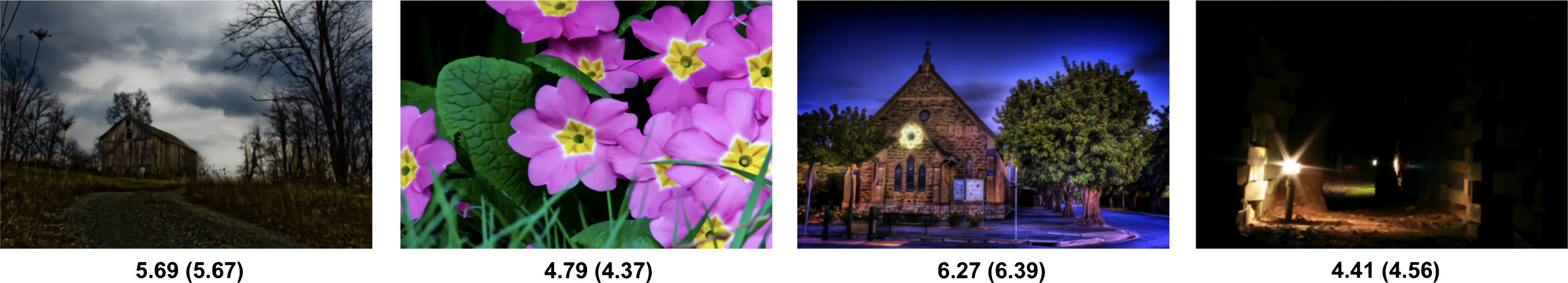
The prediction results of our AestheticNet* on the AVA dataset and the prediction (and ground truth) scores are displayed below each picture.

As we can see, the predicted score of AestheticNet* on the test image is closer to the actual score. For example, the real aesthetic score of the first image is 5.67, and the prediction result of the model is 5.69. The ground truth score of the second image is 4.37, and the prediction result of the model is 4.79. The first and third images in Figure 9 are considered high-quality images by the photographer, and the model also predicts high-quality images. The second and fourth images are classified by the photographer as low-quality images, and the model also predicts them as low-quality images. Judging from human intuitive experience, the composition and color of the first and third pictures are obviously better than those of the second and fourth pictures, and the aesthetic feeling is indeed much better. In this respect, the predictive effect of the model conforms to human aesthetic standards.

4.8 Experiments on the TID2013 dataset

To further verify the effectiveness of the AestheticNet obtained through the customized P-DARTS search algorithm and the improvement strategy introduced in this paper, we also chose the TID2013 dataset for experiments. We divide the TID2013 dataset into the training set and the validation set at a ratio of 4:1. We first train AestheticNet* on this training set and then perform verification on the test set. The experimental results are shown in Table 7, and the results are best indicated in bold font. It is worth mentioning that NIMA is pre-trained on the ImageNet dataset, while the AestheticNet* model is searched on the AVA dataset and trains from scratch on the TID2013 dataset. However, when transferred to the TID2013 dataset, the performance of AestheticNet* is comparable to the NIMA model.

Table 7
Performance comparison with other methods on TID2013 dataset

Model Name LCC(mean) SROCC(mean) LCC(var) SROCC(var) EMD Pretrained

Kim et al. [34] 0.80 0.80 - - - Y

NIMA(MobileNet) [14] 0.782 0.698 0.209 0.181 0.105 Y

NIMA(Inception-V2) [14] 0.827 0.750 0.470 0.468 0.064 Y

NIMA(VGG) [14] 0.941 0.944 0.538 0.557 0.054 Y

AestheticNet* 0.834 0.763 0.61 0.53 0.061 N

Model Name	LCC(mean)	SROCC(mean)	LCC(var)	SROCC(var)	EMD	Pretrained
Kim et al. [34]	0.80	0.80	-	-	-	Y
NIMA(MobileNet) [14]	0.782	0.698	0.209	0.181	0.105	Y
NIMA(Inception-V2) [14]	0.827	0.750	0.470	0.468	0.064	Y
NIMA(VGG) [14]	0.941	0.944	0.538	0.557	0.054	Y
AestheticNet*	0.834	0.763	0.61	0.53	0.061	N

The pictures in Figure 10 are all selected from the TID2013 dataset. The first picture is the original picture without any distortion operation, and the following pictures are all different degrees and types of distortion operations performed on the original picture. We use our trained aesthetic model to rate these pictures and compare them with the actual rating results. It can be seen that the predicted effect of our model is very close to the actual artificial scoring result. The numerical indicators and visualization results demonstrate the effectiveness of AestheticNet obtained through search and the optimization strategies introduced in this paper.

Fig. 10

The prediction results of our AestheticNet* on the TID2013 dataset and the prediction (and ground truth) scores are displayed below each picture.

5 Conclusion

In this paper, we explore the combination of neural architecture search and computational aesthetics for the first time. Through automated search, the difficulty of manually designing the aesthetic network and the problem of repeated verification in the design process are solved. We design a customized search strategy, obtain a baseline model suitable for aesthetic tasks through search, and make a series of improvements on this model, and get promising results on common aesthetic datasets. We hope that the design and improvement of our aesthetic baseline model will inspire other researchers to pay more attention to the design of aesthetic feature extraction networks. In our future research work, we will try to deploy the model to mobile devices to realize the practical value of our research. In addition, we will further design the search space and introduce more convolution operations with stronger feature extraction capabilities. For example, Involution convolution, Group convolution, SE attention module, etc. On the other hand, we will continue to investigate and add more light-weighted and effective modules to further improve the performance of our baseline aesthetic network.

Footnotes

Acknowledgments

This work is supported by the project “Construction and Intelligent Applications of Industrial Knowledge Graph for Domain Specific Scenarios” (Project#:TC2008032).

References

, Liu

and Wen Chen

, A-lamp: Adaptive layout-aware multi-patch deep convolutional neural network for photo aesthetic assessment, in: Proceedings of the IEEE Conference on Computer Vision and Pattern Recognition (2017), 4535–4544.

Wang

, Deng

, Li

and Xu

, Image aesthetic assessment based on perception consistency, in: Pattern Recognition and Computer Vision - Second Chinese Conference, PRCV 2019, Xi’an, China, November 8-11, 2019, Proceedings, Part II, (2019), 303–315.

Chen

, Zhang

, Zhou

, Lei

, Xu

, Zheng

and Fan

, Adaptive fractional dilated convolution network for image aesthetics assessment, in: Conference on Computer Vision and Pattern Recognition, CVPR 2020, (2020), 14102–14111.

Shu

, Li

, Liu

and Xu

, Learning with privileged information for photo aesthetic assessment, Neurocomputing 404 (2020), 304–316.

Zhang

, Gao

, He

and Lu

, MSCAN: multimodal selfand-collaborative attention network for image aesthetic prediction tasks, Neurocomputing 430 (2021), 14–23.

Zoph

and Le

Q.V.

, Neural architecture search with reinforcement learning, in: International Conference on Learning Representations, ICLR, (2017).

and Koltun

, Multi-scale context aggregation by dilated convolutions, in: Y. Bengio, Y. LeCun (Eds.), International Conference on Learning Representations, ICLR, (2016).

Chollet

, Xception: Deep learning with depthwise separable convolutions, in: Conference on Computer Vision and Pattern Recognition, CVPR, 2017, 1800–1807.

Woo

, Park

, Lee

and Kweon

I.S.

, CBAM: convolutional block attention module, Proceedings of the European conference on computer vision (ECCV) 11211 (2018), 3–19in.

10.

Datta

, Joshi

, Li

and Wang

J.Z.

, Studying aesthetics in photographic images using a computational approach, A. Leonardis, H. Bischof, A. Pinz (Eds.), European Conference on Computer 3953 (2006), 288–301in.

11.

Tang

, Luo

and Wang

, Content-based photo quality assessment, IEEE Trans Multim 15(8) (2013), 1930–1943.

12.

Guo

, Xiong

, Huang

and Li

, Image esthetic assessment using both hand-crafting and semantic features, Neurocomputing 143 (2014), 14–26.

13.

Chamaret

and Urban

, No-reference harmony-guided quality assessment, in: Conference on Computer Vision and Pattern Recognition, CVPR, IEEE Computer Society (2013), 961–967.

14.

Talebi

and Milanfar

, Nima: Neural image assessment, IEEE Transactions on Image Processing 27(8) (2018), 3998–4011.

15.

, Zhu

, Zhao

, Ding

, Jiang

and Tan

, Personality driven multi-task learning for image aesthetic assessment, in: IEEE International Conference on Multimedia and Expo, ICME, (2019), 430–435.

16.

Pan

, Wang

and Jiang

, Image aesthetic assessment assisted by attributes through adversarial learning, in: Conference on Artificial Intelligence, AAAI (2019), 679–686.

17.

, Zhu

, Zhao

, Ding

and Lin

, Personality-assisted multi-task learning for generic and personalized image aesthetics assessment, IEEE Trans Image Process 29 (2020), 3898–3910.

18.

Takimoto

, Omori

and Kanagawa

, Image aesthetics assessment based on multi-stream CNN architecture and saliency features, Appl Artif Intell 35(1) (2021), 25–40.

19.

Zoph

, Vasudevan

, Shlens

and Le

Q.V.

, Learning transferable architectures for scalable image recognition, in: Conference on Computer Vision and Pattern Recognition, CVPR, (2018), 8697–8710.

20.

Real

, Aggarwal

, Huang

and Le

Q.V.

, Regularized evolution for image classifier architecture search, in: Conference on Artificial Intelligence, AAAI, (2019), 4780–4789.

21.

Liu

, Simonyan

and Yang

, DARTS: differentiable architecture search, in: International Conference on Learning Representations, ICLR, (2019).

22.

Chen

, Xie

, Wu

and Tian

, Progressive differentiable architecture search: Bridging the depth gap between search and evaluation, in: International Conference on Computer Vision, ICCV, (2019), 1294–1303.

23.

Murray

, Marchesotti

and Perronnin

, AVA: A large-scale database for aesthetic visual analysis, in: Conference on Computer Vision and Pattern Recognition (2012), 2408–2415.

24.

Ponomarenko

N.N.

, Ieremeiev

, Lukin

V.V.

, Egiazarian

K.O.

, Jin

, Astola

, Vozel

, Chehdi

, Carli

, Battisti

and Kuo

C.J.

, Color image database TID2013: peculiarities and preliminary results, in: European Workshop on Visual Information Processing, EUVIP, (2013), 106–111.

25.

Kao

, He

and Huang

, Deep aesthetic quality assessment with semantic information, IEEE Trans Image Process 26(3) (2017), 1482–1495.

26.

Wang

and Shen

, Deep cropping via attention box prediction and aesthetics assessment, in: International Conference on Computer Vision, ICCV, (2017), 2205–2213.

27.

Meng

, Gao

, Shi

, Zhu

and Zhu

, Mlans: Image aesthetic assessment via multi-layer aggregation networks, in: Eighth International Conference on Image Processing Theory, Tools and Applications, IPTA, (2018), 1–6.

28.

Zhang

, Zhu

, Xu

, Liu

, Xiao

and Tillo

, Visual aesthetic understanding: Sample-specific aesthetic classification and deep activation map visualization, Signal Process Image Commun 67 (2018), 12–21.

29.

Zhang

, Gao

, Lu

, Yu

and He

, Fusion global and local deep representations with neural attention for aesthetic quality assessment, Signal Process Image Commun 78 (2019), 42–50.

30.

Sheng

, Dong

, Chai

, Wang

, Zhou

, Huang

, Hu

, Ji

and Ma

, Revisiting image aesthetic assessment via self-supervised feature learning, in: Conference on Artificial Intelligence, AAAI, (2020), 5709–5716.

31.

Sherashiya

, Shikkenawis

and Mitra

S.K.

, Image aesthetic assessment: A deep learning approach using class activation map, Computer Vision and Image Processing - 5th International Conference, CVIP 1377 (2020), 87–99in.

32.

Wang

, Wang

, Yamasaki

and Aizawa

, Aspect-ratiopreserving multi-patch image aesthetics score prediction, in: Conference on Computer Vision and Pattern Recognition Workshops, CVPR, (2019), 1833–1842.

33.

, Wang

, Zhang

and Jiang

, Spatial attentive image aesthetic assessment, in: International Conference on Multimedia and Expo, ICME, (2020), 1–6.

34.

Kim

, Zeng

, Ghadiyaram

, Lee

, Zhang

and Bovik

A.C.

, Deep convolutional neural models for picture-quality prediction: Challenges and solutions to data-driven image quality assessment, IEEE Signal Process Mag 34(6) (2017), 130–141.

Research on aesthetic models based on neural architecture search

Abstract

Keywords

1 Introduction

2 Related work

2.1 Computational aesthetics

2.2 Network architecture search

3.1 Preliminary

4.1 Dataset

4.2.1 Accuracy

4.3 NAS and aesthetic tasks

Table 4 Comparisons on the attention mechanism Model Name LCC(mean) SROCC(mean) LCC(var) SROCC(var) EMD Accuracy AestheticNet 0.623 0.603 0.211 0.214 0.052 78.3% AestheticNet+CBAM 0.664 0.678 0.216 0.217 0.051 79.7%

Table 5 Comparisons on adaptive pooling Model Name LCC(mean) SROCC(mean) LCC(var) SROCC(var) EMD Accuracy AestheticNet 0.623 0.603 0.211 0.214 0.052 78.3% AestheticNet+Adaptive Pooling 0.643 0.666 0.213 0.215 0.052 79.6%

Footnotes

Acknowledgments

References

Table 4
Comparisons on the attention mechanism

Model Name LCC(mean) SROCC(mean) LCC(var) SROCC(var) EMD Accuracy

AestheticNet 0.623 0.603 0.211 0.214 0.052 78.3%

AestheticNet+CBAM 0.664 0.678 0.216 0.217 0.051 79.7%

Table 5
Comparisons on adaptive pooling

Model Name LCC(mean) SROCC(mean) LCC(var) SROCC(var) EMD Accuracy

AestheticNet 0.623 0.603 0.211 0.214 0.052 78.3%

AestheticNet+Adaptive Pooling 0.643 0.666 0.213 0.215 0.052 79.6%