An ensemble deep neural network approach for predicting TOC concentration in lakes along the middle-lower reaches of Yangtze River

Abstract

In recent years, lakes pollution has become increasingly serious, so water quality monitoring is becoming increasingly important. The concentration of total organic carbon (TOC) in lakes is an important indicator for monitoring the emission of organic pollutants. Therefore, it is of great significance to determine the TOC concentration in lakes. In this paper, the water quality dataset of the middle and lower reaches of the Yangtze River is obtained, and then the temperature, transparency, pH value, dissolved oxygen, conductivity, chlorophyll and ammonia nitrogen content are taken as the impact factors, and the stacking of different epochs’ deep neural networks (SDE-DNN) model is constructed to predict the TOC concentration in water. Five deep neural networks and linear regression are integrated into a strong prediction model by the stacking ensemble method. The experimental results show the prediction performance, the Nash-Sutcliffe efficiency coefficient (NSE) is 0.5312, the mean absolute error (MAE) is 0.2108 mg/L, the symmetric mean absolute percentage error (SMAPE) is 43.92%, and the root mean squared error (RMSE) is 0.3064 mg/L. The model has good prediction performance for the TOC concentration in water. Compared with the common machine learning models, traditional ensemble learning models and existing TOC prediction methods, the prediction error of this model is lower, and it is more suitable for predicting the TOC concentration. The model can use a wireless sensor network to obtain water quality data, thus predicting the TOC concentration of lakes in real time, reducing the cost of manual testing, and improving the detection efficiency.

Keywords

Water quality monitoring total organic carbon (TOC) concentration ensemble learning deep learning

1 Introduction

With the rapid development of the economy, environmental pollution is becoming increasingly serious, so water quality monitoring has become very important [1]. Water quality monitoring is a process of evaluating water quality by monitoring and determining the types of pollutants in water, the concentration of pollutants and the change in different pollutants. The scope of water quality monitoring is very wide, including uncontaminated and contaminated natural water (river, lake, sea and underground water) and all kinds of industrial drainage. The main monitoring items can be divided into two categories: one is a comprehensive index reflecting water quality, such as temperature, chroma, turbidity, pH value, conductivity, suspended matter, dissolved oxygen, chemical oxygen demand and biochemical oxygen demand [2]. The other is toxic substances, such as phenol, cyanogen, arsenic, lead, chromium, cadmium, mercury and organic pesticides. To evaluate the water quality of rivers and oceans more objectively, in addition to the above monitoring items, flow velocity and water flow are sometimes measured [3, 4].

The emission of organic pollutants is one of the main causes of lake pollution. The comprehensive index of organic pollution mainly includes chemical oxygen demand and total organic carbon (TOC) concentration [5 –7]. TOC in inland waters is an important part of the global carbon cycle. As a channel between the terrestrial environment and the ocean, lakes and rivers control the emission of greenhouse gases and store carbon in their sediments. In the function of aquatic ecosystem, TOC concentration plays an important role by affecting the physical and chemical properties of water, and then affecting the structure of biological community [8]. For example, TOC affects water acidity, dissolved oxygen level, water color, light penetration and thermal penetration, thereby regulating the development of thermal stratification and anoxia. TOC is also closely related to nutrients, which together affect the species distribution of fish and the habitat availability of primary producers (bacteria and algae), thus affecting the productivity of aquatic ecosystems. In addition, TOC also affects the transportation and storage of metal and organic pollutants, the growth of toxic algae and the related costs of drinking water treatment [9]. Therefore, in the study of environmental science, it is very important to monitor the TOC concentration in aquatic ecosystem, especially for the lakes in densely populated and economically active areas.

Traditional water quality monitoring technologies are mainly physical and chemical monitoring technologies, including chemical methods, electrochemical methods, atomic absorption spectrometry, ion-selective electrode methods, ion chromatography, gas chromatography, and plasma emission spectrometry [10]. In recent years, biological monitoring, remote sensing monitoring and wireless sensor network monitoring have also been applied to monitor water quality [11 –13]. Especially with the development of wireless sensor networks, the data acquired by various sensors are transmitted to the server in real time, which can monitor the water quality changes in real time. It is more efficient and inexpensive than traditional artificial physical and chemical testing [14, 15].

In recent years, machine learning and deep learning have been widely used in various fields of environmental science and has made many achievements. Considering the weather of the previous day, taking wind field, temperature and air pollution concentration as the input of the model, Sayeed et al. developed a deep convolutional neural network model to predict the ozone concentration 24 hours in advance. The model has been trained to have a better performance in predicting the next day’s 24-hour ozone concentration [16]. To better control and manage the harbor water quality of New York City and other coastal cities, a deep learning model was proposed for water quality prediction. The model combined deep matrix decomposition and a deep neural network, which can solve the sparse matrix problem more intelligently and predict the BOD value more accurately. To test its effectiveness, 32,323 water samples were used to study the port water in New York City. The results show that compared with the traditional matrix completion method, the RMSE of this method is reduced by 11.54%–17.23%, and compared with the traditional machine learning algorithm, the RMSE is reduced by 19.20%–25.16%[17]. Pudashine et al. proposed a rainfall retrieval deep learning model based on a long short-term memory (LSTM) model architecture, which was trained with data provided by mobile network operators. The experimental results show that the coefficient of determination (R-2) for rainfall prediction increases from 0.86 to 0.97, and the observed total rainfall estimates significantly improved [18]. Chen et al. endeavored to compare the water quality prediction performance of 10 learning models (7 traditional and 3 ensemble models) using big data (33,612 observations) from the major rivers and lakes in China from 2012 to 2018 based on the precision, recall, F1-score, and weighted F1-score and explored the potential key water parameters for future model prediction. The results showed that bigger data can improve the performance of learning models in the prediction of water quality [19].

For predicting TOC concentration using machine learning and deep learning, there are also some preliminary researches [20]. Meyer-Jacob et al. proposed an orthogonal partial least squares model (PLS) to infer TOC concentrations in lakes of northern Europe and North America. Based on the surface water data of 345 Arctic to north temperate lakes in Canada, Greenland, Sweden and Finland, the model used the visible near infrared (VNIR) spectra of lake sediments to predict the TOC concentration of lakes in southern Ontario and Scotland. The experimental results showed that the R-2 of the model cross validation is 0.57 [21]. Shalaby et al. studied the TOC concentration in Taranaki Basin, five machine learning techniques, namely Bayesian regularization for feed-forward neural networks (BRNNs), random forest (RF), support vector machine (SVM) for regression, linear regression (LR) and Gaussian process regression (GPR), were employed for prediction of TOC, the results showed that the prediction performance of random forest is the best, and achieved the R-2 value of 0.964 [22]. Handhal et al. evaluated the use of three machine learning models namely, RF, rotation forest (rF), K-nearest neighbors (KNN) to estimate TOC based on conventional well logs data. Results indicated the KNN was the best followed by RF and then rF. The study confirmed the ability of machine learning models for building efficient model for estimating TOC [23]. Lu et al. constructed TOC prediction model by combining abnormal sample elimination, spectral feature transformation and feature wavelength extraction to predict the TOC concentration in intertidal sediments, and used PLS, least squares support vector machine (LSSVM) and BP Neural Network (BPNN) to model and predict sediment TOC concentration, the experimental results showed that the prediction accuracy of LSSVM is the highest, with the R-2 value of 0.86 [24]. The above researches are helpful exploration of machine learning and deep learning in the prediction of TOC concentration. However, the research areas of these studies are generally small, while these areas are sparsely populated and economic production activities are not active, which means almost uncontaminated; on the other hand, the prediction accuracy of the above methods needs to be improved.

Ensemble learning is a meta method that combines several machine learning models into a whole prediction model. The prediction performance of this model is usually better than that of the single models [25, 26]. Therefore, ensemble learning method can greatly improve the prediction accuracy. In recent years, ensemble learning has been widely used in various fields of research. Wang et al. combined an adaptive neuro-fuzzy inference system (ANFIS) with two metaheuristic methods of biogeography, the ensemble methods were more effective than ANFIS in the study area [27]. Bui et al. provided an approach for flash flood susceptibility modeling based on a feature selection method (FSM) and tree based ensemble methods, and compared to a conventional rule based method, the approach gave more accurate predictive results [28]. In the field of industry electronic, Zhao et al. predicted the eddy current losses of metal fasteners in rotor slots of a large nuclear steam turbine generator, the ensemble model presented better performance [29].

In this paper, to improve the prediction precision of the TOC concentration in lakes, a new ensemble model is proposed, named the stacking of different epochs’ deep neural networks (SDE-DNN) model. By taking temperature, transparency, pH value, dissolved oxygen, conductivity, chlorophyll and ammonia nitrogen as inputs of the model, the TOC concentration is predicted. Compared with other models listed, the superiority of the proposed model in predicting the TOC concentration in water is verified. This method can use other indexes obtained by sensor networks to predict the TOC concentration of lakes in real time, while avoiding excessive human participation, improving efficiency and reducing testing cost.

Fig. 1

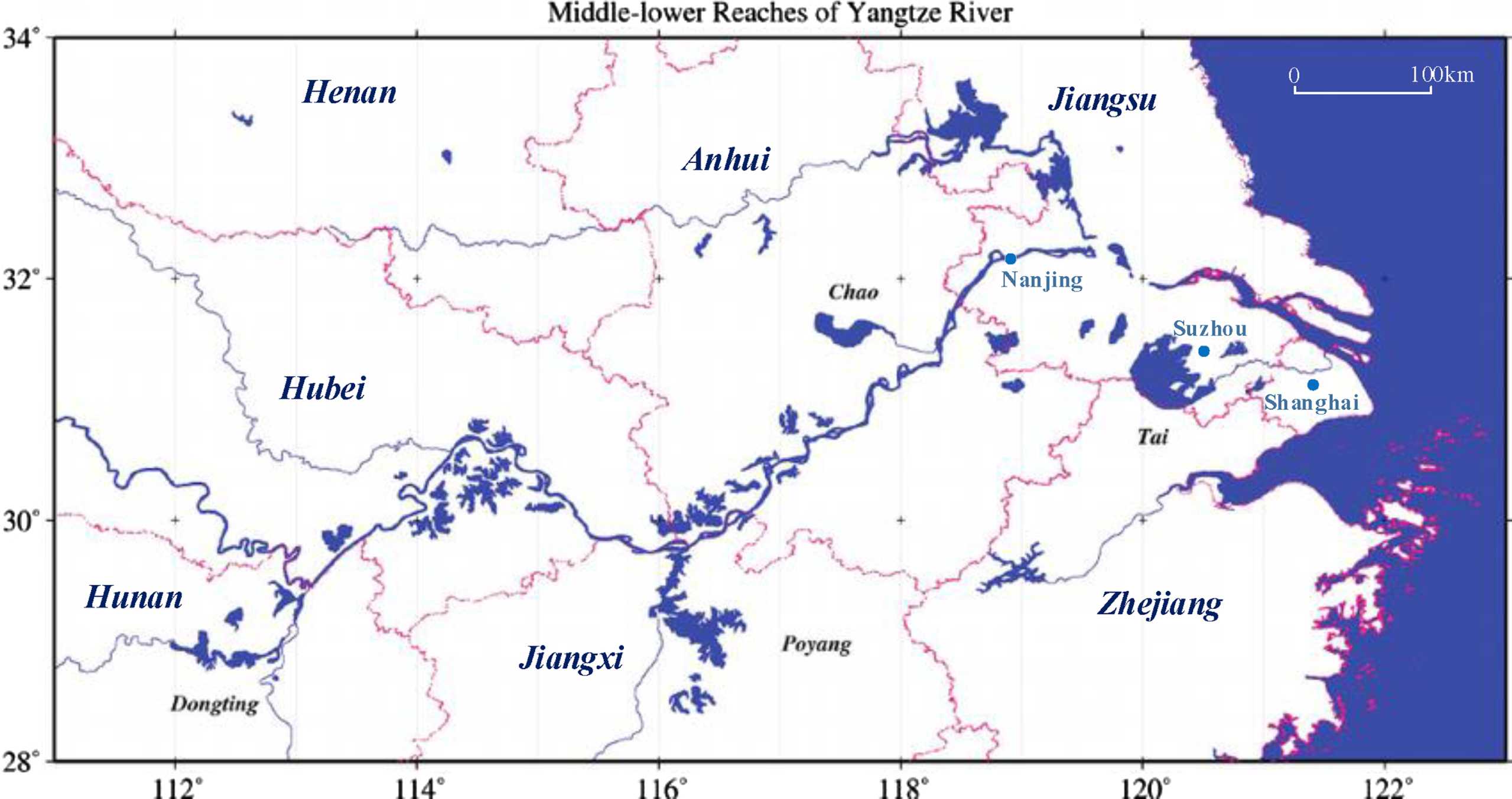
Distribution of lakes in the middle and lower reaches of the Yangtze River.

2 Materials and methods

2.1 Description of the study area

There are more than 24,800 lakes in China, including 2,800 natural lakes with an area of more than 1 square kilometer. Although the number of lakes is large, the regional distribution is very uneven. In general, the eastern monsoon region, especially the middle and lower reaches of the Yangtze River, is the largest freshwater lake area in China [30, 31].

The geographical range of the middle and lower reaches of the Yangtze River is between 28°45’ –33° 25’ N and 111°17’ –123°25’ E. There are 642 lakes with a total area of 15794.6 km². The distribution of lakes in the middle and lower reaches of the Yangtze River is shown in Fig. 1. Due to the small drop of water level and small flow velocity in plain area, the flow direction is uncertain due to the height control of water conservancy project and the influence of gate opening and closing and water diversion and drainage. In addition to the local surface water runoff, the rivers and lakes also bear the water from the upper 15 provinces with an area of about 2 million km². In flood years, the middle and lower reaches of the Yangtze River are the flood corridors of the upstream water systems. Facing the ocean, they are easily attacked by storm rain and storm surge from Taiwan, which often lead to external flood, internal waterlogging or concurrent flood of external flood and internal waterlogging. In drought years, there is little water from the upper reaches, which often leads to serious drought and worsens the water quality of rivers and lakes. In addition, some rivers have high sediment concentration, channel siltation, river bed slope slowing down, and reservoir sediment deposition makes sediment absorb pollutants, which aggravates the pollution of water environment and increases the difficulty of development and utilization of water resources.

Meanwhile, the middle and lower reaches of the Yangtze River are important industrial production bases in China. The main cities in the region include Shanghai, Nanjing, Suzhou and other first tier cities, and the total population of the region is about 74,047,100. Dense population and frequent human activities further aggravate the water pollution situation in this area, and the importance of water quality monitoring is self-evident.

The Nanjing Institute of Geography and Lakes of the Chinese Academy of Sciences (CAS) has set up a large number of water quality monitoring stations in the main lakes in the middle and lower reaches of the Yangtze River through the construction of the “scientific database” of the Chinese Academy of Sciences, the “China Lake database” of the 10th 5-year plan, the “China Lake Science Professional Database” of the 11th 5-year plan, and the “key database of science and technology data resource integration and sharing project” of the 12th 5-year plan. Table 1 shows the monitoring stations in the main lakes in the middle and lower reaches of the Yangtze River.

Table 1
Large lakes in the middle and lower reaches of the Yangtze River

Province Lake name

Hunan Dong Lake, Dongting Lake, Liuye Lake, Shanpo Lake, Datong Lake, Huanggai Lake, Beimin Lake; Maoli Lake, Bajiao Lake, Nan Lake

Hubei/Anhui Longgan Lake

Hubei Liangzi Lake, Haikou Lake, Futou Lake, Lu Lake, Hong Lake, Nan Lake, Liulang Lake, Huangshan Lake, ShanShan Lake, Houguan Lake, Shangshe Lake, Shanglu Lake, Tangxun Lake, Taibai Lake, Bao’an Lake, Yezhu Lake

Jiangxi Poyang Lake, Zhu Lake, Yao Lake, Xinmiao Lake, Sai Lake, Taibo Lake, Chi Lake, Nanbei Lake, Chenjia Lake, Niujun Lake

Jiangsu Cheng Lake, Shijiu Lake, Changdang Lake, Yuandang Lake, Yangcheng Lake

Anhui Chao Lake, Nanyi Lake, Caizi Lake, Huangda Lake

Shanghai Dingshan Lake

Province	Lake name
Hunan	Dong Lake, Dongting Lake, Liuye Lake, Shanpo Lake, Datong Lake, Huanggai Lake, Beimin Lake; Maoli Lake, Bajiao Lake, Nan Lake
Hubei/Anhui	Longgan Lake
Hubei	Liangzi Lake, Haikou Lake, Futou Lake, Lu Lake, Hong Lake, Nan Lake, Liulang Lake, Huangshan Lake, ShanShan Lake, Houguan Lake, Shangshe Lake, Shanglu Lake, Tangxun Lake, Taibai Lake, Bao’an Lake, Yezhu Lake
Jiangxi	Poyang Lake, Zhu Lake, Yao Lake, Xinmiao Lake, Sai Lake, Taibo Lake, Chi Lake, Nanbei Lake, Chenjia Lake, Niujun Lake
Jiangsu	Cheng Lake, Shijiu Lake, Changdang Lake, Yuandang Lake, Yangcheng Lake
Anhui	Chao Lake, Nanyi Lake, Caizi Lake, Huangda Lake
Shanghai	Dingshan Lake

These stations use artificial physical and chemical detection and automatic monitoring to obtain data. The TOC concentration can only be detected by artificial physical and chemical stations. This paper focuses on the middle and lower reaches of the Yangtze River, using the water quality performance data measured by artificial physical and chemical detection to predict the TOC concentration in lakes by machine learning methods.

2.2 Sample collection and testing methods

To verify the prediction model of the TOC concentration in water, the monitoring data of water quality in the middle and lower reaches of the Yangtze River from 2007 to 2009 were obtained from the Lake-Basin thematic database in the middle and lower reaches of the Yangtze River (http://www.lakesci.csdb.cn/front/detail-lake2014$zdhpszrgjc?id=2000) of the China lake database. The lakes as data sources are shown in Table 1. A total of 272 water quality monitoring samples were selected from the above database as the samples of this experiment. The samples were obtained by water quality monitoring stations around the main lakes along the Yangtze River. The water quality samples were collected from 74 lakes from October 11, 2007 to April 9, 2009. The number of water quality samples collected from each lake ranged from 1 to 25. Detailed data can be found in Tables S2 in the Appendix A.

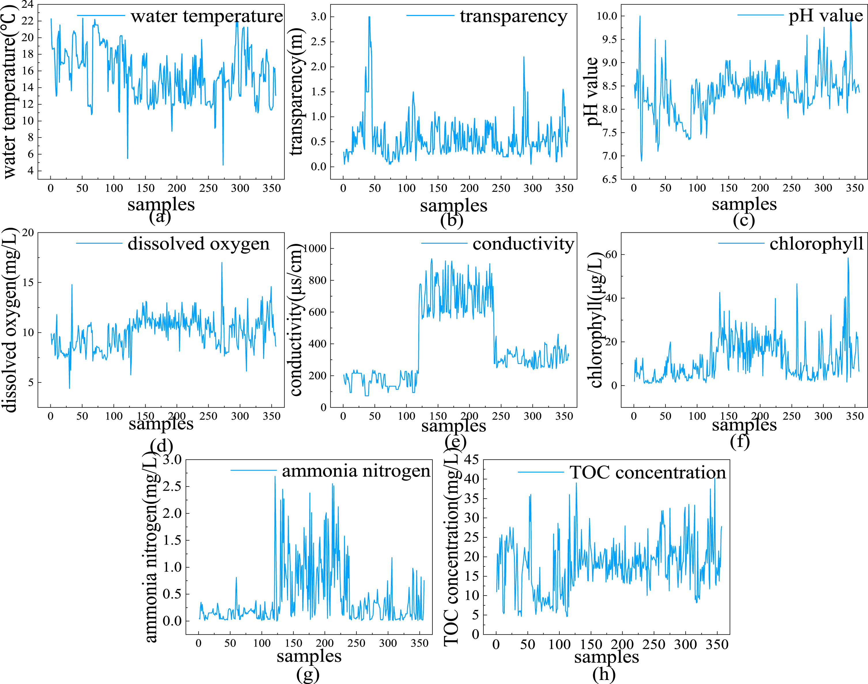
According to the data obtained by wireless network, water temperature (°C), transparency (m), pH value, dissolved oxygen (mg/L), conductivity (μs/cm), chlorophyll (μg/L) and ammonia nitrogen (mg/L) were taken as the input to the model, and the output was the TOC concentration (mg/L). Figure 2 shows all of the water quality monitoring samples. The data come from different monitoring stations in different lakes at different times, so the values of water quality samples may be biased. In Fig. 2, the data with abnormally high DO value comes from the second monitoring station of Yuandang Lake, and the data with abnormally high chlorophyll value comes from the third monitoring station of Xinmiao Lake. The reason for the abnormality may be the deviation caused by the different geographical location of the lake or the statistical error of the monitoring station. In order to ensure the reliability of the prediction results, we remove the outliers.

Fig. 2

Water quality monitoring samples: (a) water temperature, (b) transparency, (c) pH value, (d) dissolved oxygen, (e) conductivity, (f) chlorophyll, (g) ammonia nitrogen, (h) content of TOC.

The K-means clustering method is used to divide the data into three clusters, and the number of each group is different. Synthetic Minority Oversampling Technique (SMOTE) and Adaptive Synthetic Sampling Algorithm (ADASYM) can be used to solve this problem [32]. In this paper, SMOTE is selected, therefore, a total of 357 pieces of data are finally obtained, which are divided into three groups, with 119 pieces of data in each group. The final data image is shown in Fig. 3.

Correlation analysis was conducted to the collected data samples. Figure 4 shows the correlation coefficient matrix. It can be seen that conductivity and chlorophyll have stronger positively correlation with TOC concentration under the samples, and the correlation coefficients are 0.58, and 0.45 respectively. While the temperature is stronger negatively correlated to TOC concentration with the correlation coefficient of –0.38. The correlation between transparency, pH value, dissolved oxygen, ammonia nitrogen and TOC concentration is weak, and the correlation coefficients are –0.16, 0.07, 0.25 and 0.03, respectively.

Fig. 3

Water quality monitoring samples after outliers removed: (a) water temperature, (b) transparency, (c) pH value, (d) dissolved oxygen, (e) conductivity, (f) chlorophyll, (g) ammonia nitrogen, (h) content of TOC.

Fig. 4

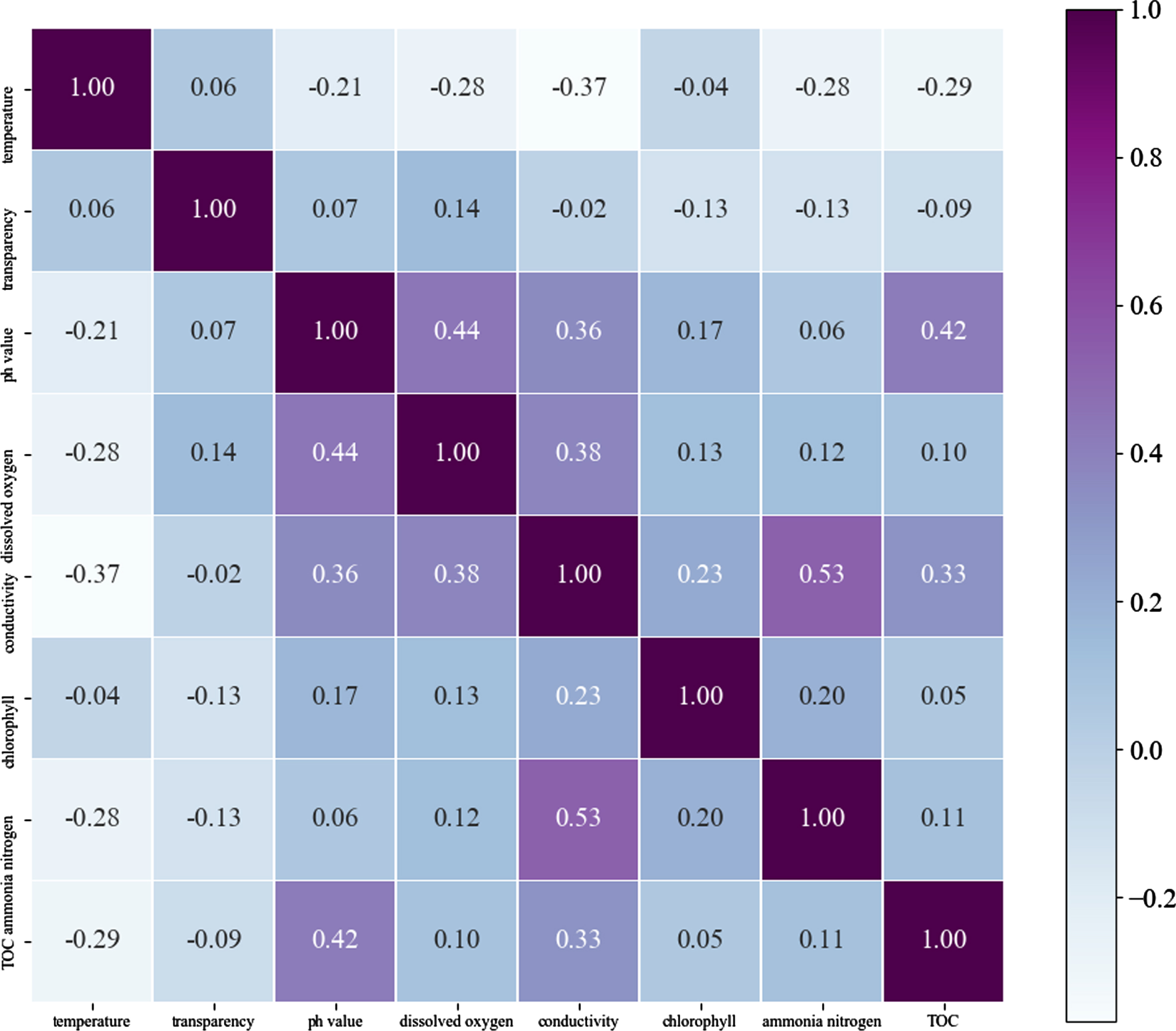
Correlation coefficient matrix of the water quality parameters.

2.3 Model description

2.3.1 Ensemble learning

Ensemble learning is a meta method that integrates multiple weak classifiers or regression models into a strong classifier or regression model. It can be used for the ensemble of classification problems, regression problems, feature selection, outlier detection, etc. [33]. Common ensemble learning methods include bagging, boosting, and stacking.

The training set of bagging’s individual weak learner is obtained by random sampling [34]. Through T random sampling iterations, we can obtain T sample sets. For these T sample sets, we can train T weak learners independently and then obtain the final strong learners through the aggregation strategy.

Boosting is a family of algorithms that can promote weak learners to strong learners [35]. The mechanism of the algorithm is to train a base learner from the initial training set and then adjust the distribution of training samples according to the performance of the base learner so that the training samples that the previous base learners trained incorrectly will receive more attention in the follow-up. Then, the next basic learner was trained based on the adjusted sample distribution; this process is repeated until the number of base learners reaches the preassigned value T, and finally, the T base learners are weighted combined.

Stacking is a typical representative ensemble learning method. It is a hierarchical ensemble model [36]. The stacking model is usually divided into two layers: a level 0 layer and a level 1 layer. Generally, the level 1 layer is called the metalayer. The learners in the level 0 layer are called base learners, and the learners in the level 1 layer are called metalearners. Stacking uses the initial training set to train the base learner and then generates a new dataset to train metalearners. In this new dataset, the output of the base learner is treated as an input sample, while the label of the initial sample is still treated as a sample label. Unlike bagging and boosting, stacking is asynchronous integration, which can integrate different types of classifiers or regression models.

2.3.2 Deep neural network

The basis of deep neural network (DNN) is artificial neural network (ANN). ANN is a mathematical model inspired by the structure and function of biological neural network [37]. It has the ability to deal with complex and nonlinear input-output relations and dimension problems, and has been widely used in various fields [38]. Figure 5(a) shows the general structure of ANN. DNN is the extension of ANN, so that its structure is similar to ANN [39, 40]. As shown in Fig. 5(b), the layers of DNN are fully connected, that is, each neuron in the previous layer must be connected with all neurons in this layer. According to different location of the layers, they can be divided into input layer, hidden layer and output layer. Generally, the first layer is the input layer, the last layer is the output layer, and the intermediate layers are hidden layers.

Fig. 5

Structures of an artificial neural network (ANN) and a deep neural network (DNN). (a) A simple example of an ANN. (b) A DNN with more layers.

DNN has also developed many variants of neural networks, such as Convolutional Neural Network (CNN) and Long Short-Term Memory (LSTM) [41 –43]. CNN is generally used to solve the problem of image recognition, while LSTM is a special recurrent neural network model. Its special structure design makes it possible to avoid the problem of long-term dependence. However, this paper focuses on regression prediction, which is a method to predict the development trend and level of dependent variables based on one or several independent variables. This trend and level of change is not only reflected in the regularity of natural changes in time series, but also in the regularity of causality between variables. Therefore, the fully connected DNN model is still a suitable choice.

2.3.3 Establishment of the neural network

When the deep neural network is used for regression prediction, the prediction results may be different due to the change in epochs of backpropagation training [44]. Therefore, this paper combines deep learning with ensemble learning and proposes the stacking of different epochs’ deep neural networks (SDE-DNN) model. The model adopts a two-layer stacking structure. The first layer uses five deep neural network models. These models are derived from the same base DNN model. The structure of the base model is shown in Fig. 6(a). Table 2 shows the information of the base DNN model.

Fig. 6

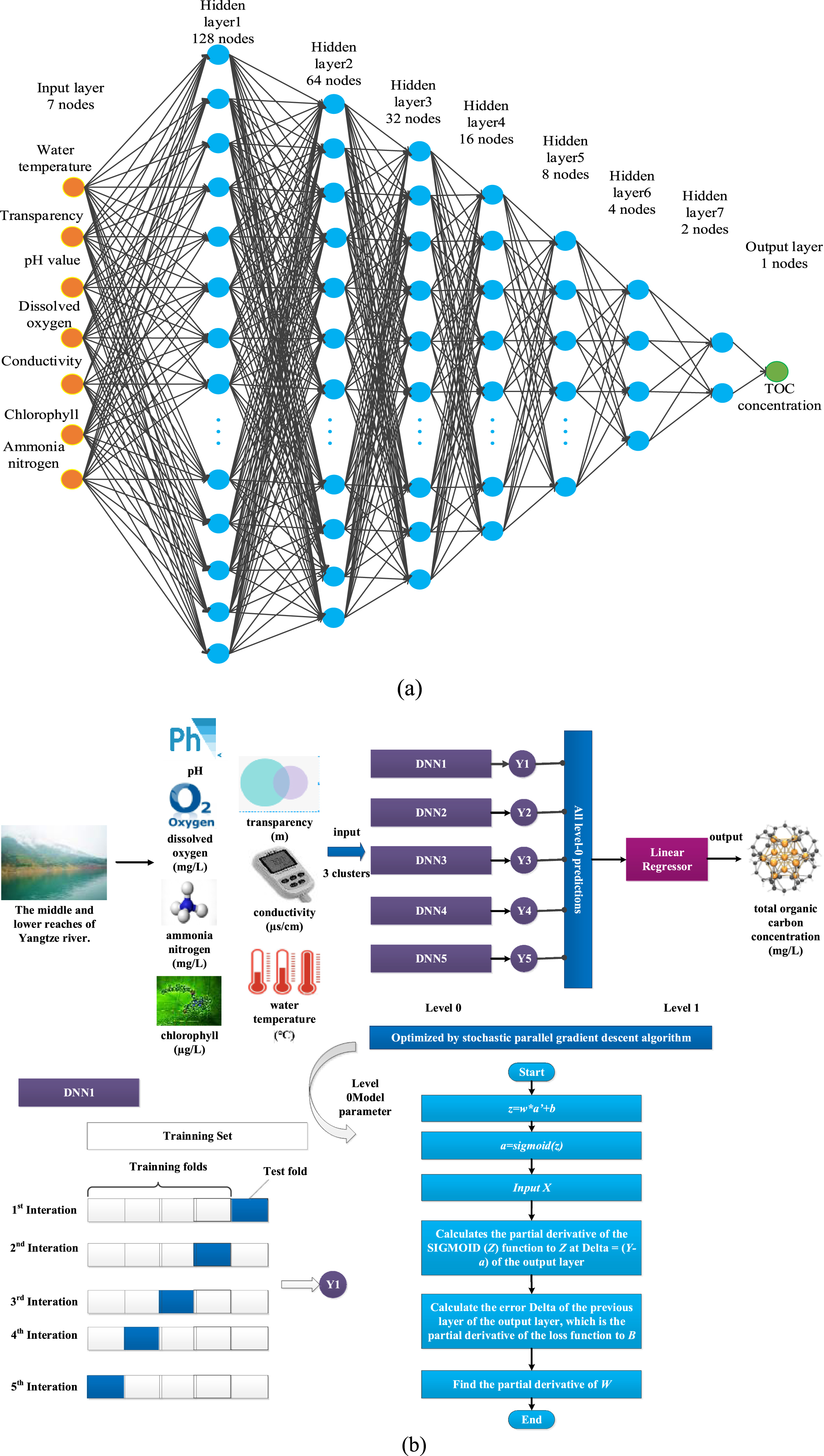
Prediction model of TOC in water based on the SDE-DNN: (a) base DNN model, (b) overall process of TOC concentration prediction in water.

The structure and parameters of the basic DNN model are determined by a large number of experiments. Here are some experimental results. Table 3 shows the prediction results of SDE-DNN models with different basic DNN models. More detailed results can be found in Section 3.4. Generally, the results of the basic DNN model used in this paper are better than other basic DNN models.

In this paper, the water temperature, transparency, pH value, dissolved oxygen, conductivity, chlorophyll and ammonia nitrogen are taken as the input to the model, and the TOC concentration in water is taken as the output of the model. Figure 6(b) shows the complete process of predicting the TOC concentration in water.

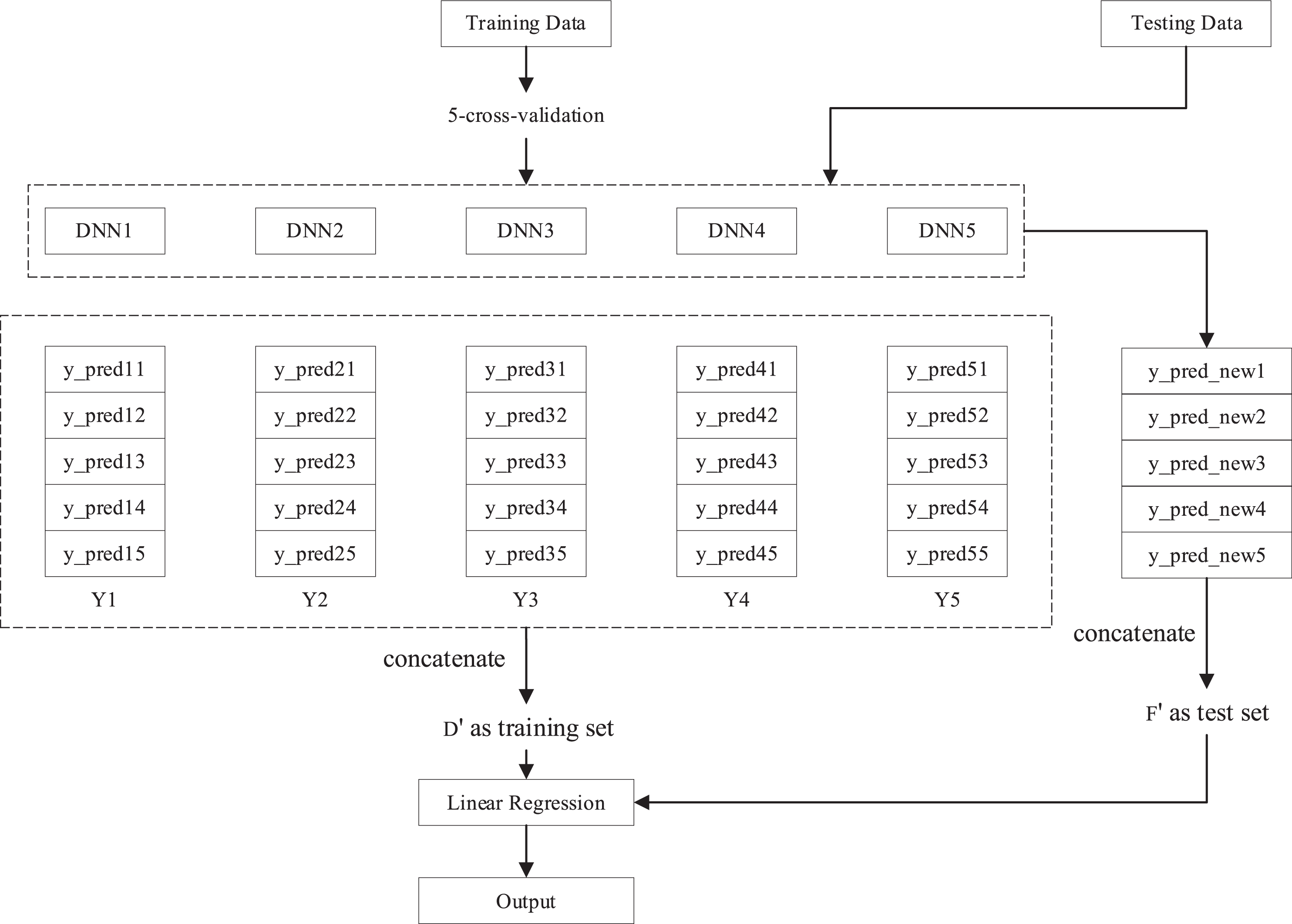
For each cluster, by setting the epochs of backpropagation training from 100 to 500 with a step size equal to 100, five deep neural network models DNN1-DNN5 are obtained. Inputting the dataset established in Section 2.2 into the 5 DNN models, then the prediction output Y1 to Y5 can be obtained. Among them, Y1 is the concatenation of the 5 prediction results (y_pred11 to y_pred15) of DNN1 after 5-fold cross validation, Y2-Y5 are calculated in the similar way.

The output Y1 to Y5 of the first layer is collected and transferred to the linear regression model of the metalayer, and the final prediction results can be obtained through calculation. The specific process is shown in Fig. 7. It can be seen that, during 5-fold validation, each DNN model generate 5 results, such as y_pred11 to y_pred15. These results concatenate to a feature Y1, and for 5 DNN models, 5 features Y1 to Y5 can be concatenated to a new training set D′. Similarly, 5 test set y_pred_new1 to y_pred_new5 can be obtained by inputting original test set into 5 DNN models, and a new test set F′ can be concatenated by these new test sets.

Table 3

Prediction results of different DNN models

Base DNN	RMSE (mg/L)	MAE (mg/L)	SMAPE	NSE
7-8-16-4-2-1	0.3321	0.2364	54.84%	0.4310
7-7-20-14-1	0.3405	0.2344	52.16%	0.4019
7-8-10-20-4-1	0.3314	0.2280	50.98%	0.4335
7-128-16-4-1	0.3158	0.2269	52.37%	0.4855
7-128-64-32-16-8-4-2-1	0.3064	0.2108	43.92%	0.5312

Table 2

Information of the base DNN model

Parameters	Value of parameters
Optimization function	’RMSProp’
Learning rate	0.001
Batch size	1
Input layer	7 nodes
Number of hidden layers	8
Hidden layer 1	128 nodes, ’ReLU’
Hidden layer 2	64 nodes, ’ReLU’
Hidden layer 3	32 nodes, ’ReLU’
Hidden layer 4	16 nodes, ’ReLU’
Hidden layer 5	8 nodes, ’ReLU’
Hidden layer 6	4 nodes, ’ReLU’
Hidden layer 7	2 nodes, ’ReLU’
Output layer	1 nodes, ’linear’

Fig. 7

Training and testing process of the SDE-DNN model.

The details of the algorithm are as follows:

Algorithm:

Input: Water quality monitoring dataset with 272 samples:

K ={ (x₁, y₁) , (x₂, y₂) , ⋯ , (x₂₇₂, y₂₇₂) }

SDE-DNN model:

Level 0 layer: 5 base DNN model λ₁, λ₂, ⋯ , λ₅

Metalayer: Linear regression model λ

Steps:

Step 1: The data set is clustered into three cluster, C1, C2, C3, then the SMOTE method is used to solve the imbalance of data categories. Finally, each cluster has 119 pieces of data.

Step 2: For each cluster, the cluster is divided into two sets, 71 pieces of data (60%) as the training set

D = {(x_{1}^{D}, y_{1}^{D}), (x_{2}^{D}, y_{2}^{D}), \dots, (x_{71}^{D}, y_{71}^{D})}

, 48 pieces of data (40%) as the testing set

F = {(x_{1}^{F}, y_{1}^{F}), (x_{2}^{F}, y_{2}^{F}), \dots, (x_{48}^{F}, y_{48}^{F})}

Step 3: Five basic DNN models are used to train the training set. For a basic DNN model, for example DNN1, is conducted 5-fold cross validation. For 71 pieces of data of training set, the folding size of each fold is 14, 14, 14, 14, 15. The folding sizes are nearly the same, which has little influence on the final experimental results. After 5-fold training, the 5 test results are integrated into a new feature Y1, and 5 DNN models can generate 5 features Y1-Y5. Finally, a new training set D′ of 5 × 71 is obtained as the input of metalayer.

Step 4: 5 test set y_pred_new1 to y_pred_new5 can be obtained by inputting original test set into 5 DNN models, and a new test set F′ can be concatenated by these new test sets.

Step 5: The regression model h′ is obtained by using the linear regression model of metalayer, h′ = λ (D′).

Output:H (x) = h′ (F′)

3 Experiment and results

3.1 Experimental conditions

The computer specification used in this experiment is a dual-channel Intel E52690v2 CPU and 128 GB DDR-RAM. The programming language is Python, and the model used is the SDE-DNN model built in Section 2.3.3. The data and code for the paper are uploaded to Github, and available on https://github.com/kerlansherry/TOC_prediction.

3.2 Min-max normalization

To eliminate the difference in magnitude of data characteristics, this paper uses min-max normalization to process the sample data and normalize the data to the interval of [–1,1], as shown in Equation (1), $x_{i}^{'} = \frac{2 (x_{i} - min)}{max - min} - 1$ (1) where, $x_{i}^{'}$ represents the normalized result, x_i represents the original data, max represents the maximum of the original data, and min represents the minimum value of the original data.

3.3 Model assessment

In this paper, MAE, SMAPE, RMSE and NSE are selected to measure the reliability and accuracy of the model prediction. MAE is the average value of the absolute errors between the observed values and the predicted values, which can be used to measure the distance between the predicted values and the observed values. SMAPE is the symmetric mean absolute percentage error. RMSE are used to measure the error of the predicted value from the observed value. For the above three metrics, the smaller their values, the higher the prediction accuracy, and the higher the ability of model to fit data. NSE is generally used to verify the results of hydrological model simulation, and its value range is from negative infinity to 1. If NSE close to 1, it means that the model has good quality and high credibility; Close to 0 indicates that the simulation results are close to the average level of the observed values, that is, the overall results are reliable, but the process simulation error is large; Far less than 0, the model is not credible. 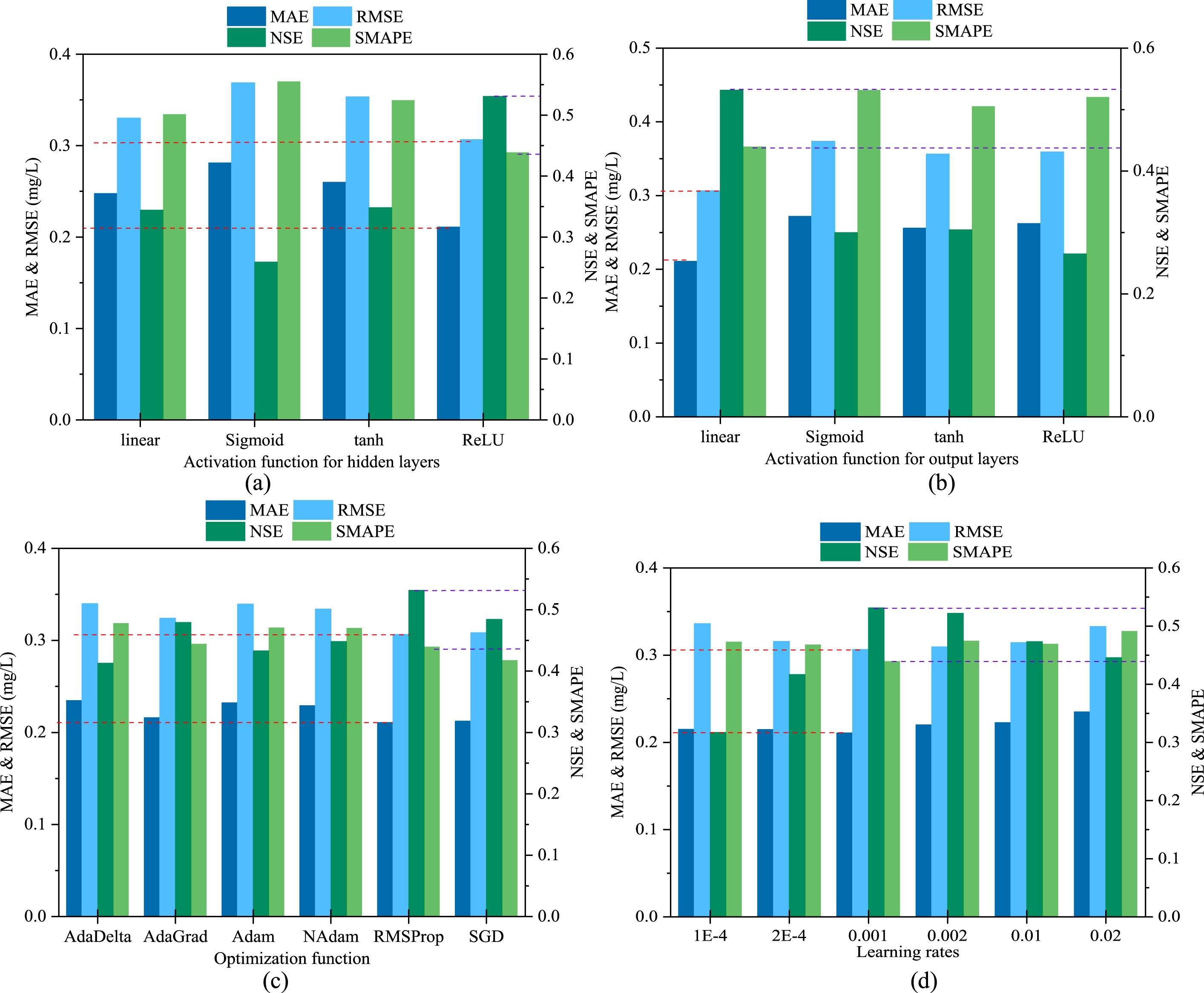The calculation formula of the four indexes is shown in Equations (5), $MAE = \frac{1}{N} \sum_{t = 1}^{N} | y_{observed}^{t} - y_{pred}^{t} |$ (2) $SMAPE = \frac{100 %}{N} \sum_{t = 1}^{N} \frac{| y_{observed}^{t} - y_{pred}^{t} |}{(| y_{observed}^{t} | + | y_{pred}^{t} |) / 2}$ (3) $RMSE = \sqrt{\frac{1}{N} \sum_{t = 1}^{N} {(y_{observed}^{t} - y_{pred}^{t})}^{2}}$ (4) $NSE = 1 - \frac{\sum {(y_{observed}^{t} - y_{pred}^{t})}^{2}}{\sum {(y_{observed}^{t} - y_{average})}^{2}}$ (5) where $y_{observed}^{t}$ represents the ith observed value, $y_{pred}^{t}$ represents the ith predicted value, y_average represents the average value of the observed values and N represents the number of samples.

Fig. 8

Experiment results of comparing with different models (a) activation functions of hidden layers (b) activation functions of output layers (c) optimization functions (d) learning rates.

3.4 Comparison of SDE-DNN models different from base DNN models

The network topology of DNN consists of the number of hidden layers, the number of neurons in the hidden layer, the activation function of the output layer and hidden layer, and the learning rate, which have a very important influence on the prediction performance of DNN. DNN with unsuitable topology will not only increase the training time but also lead to “over-fitting” or “under-fitting”.

This paper focuses on the influence of the stacking ensemble method on the DNN architecture rather than the topology of the base DNN model. Therefore, this paper does not carry out experimental research on the number of layers and neurons per layer of base DNN models.

To determine the influence of different activation functions of the hidden layer on the prediction performance of the SDE-DNN model, the linear function, sigmoid function, tanh function and ReLU function are selected as activation functions of the hidden layer of the base DNN models, and these models are tested. Other parameters remain at their default values during the test. Figure 8(a) shows the results. The prediction accuracy of the model using ReLU was the highest, with RMSE of 0.3064 mg/L and MAE of 0.2108 mg/L. The experimental results verify the advantages of the proposed model in prediction performance.

To determine the influence of different activation functions of the output layer on the network prediction performance, the linear function, sigmoid function, tanh function and ReLU function are selected as activation functions of the output layer of the base DNN models, and these models are tested. Other parameters remain at their default values during the test. Figure 8(b) shows the results. The linear model had the highest prediction accuracy, with NSE of 0.5312 and SMAPE of 43.92%. The experimental results verify the advantages of the proposed model in prediction performance.

To determine the influence of different optimization functions on network prediction performance, the AdaDelta function, AdaGrad function, Adam function, NAdam function, RMSProp function and SGD function are selected as the optimization functions of the base DNN model, and these models are tested. Other parameters remain at their default values during the test. Figure 8(c) shows the results. The model using the RMSProp function has the highest prediction accuracy, the minimum RMSE is 0.3064 mg/L, and the minimum MAE is 0.2108 mg/L. The experimental results verify the advantages of the proposed model in prediction performance.

To determine the influence of the learning rate of the backpropagation algorithm on the prediction performance of the SDE-DNN model, six different learning rates are used to establish the base DNN models for testing. Other parameters remain at their default values during the test. Figure 8(d) shows the experimental results. When the learning rate is 0.01, the minimum RMSE of the model is 0.3064 mg/L, and the minimum SMAPE is 43.92%. The experimental results verify the superiority of the proposed model in predicting TOC content in water.

In conclusion, the proposed SDE-DNN model shows the best prediction performance in all experiments, which means it is the first choice to predict the TOC concentration in lakes.

3.5 Experimental results

A method similar to grid search is used to adjust the hyperparameters of the model, so as to determine the activation function, optimization function and learning rate of the model. The specific process is presented in Section 3.4. After repeated experiments, the hidden layer activation function is set to the ReLU function, the output layer activation function is set to the linear function, the optimization function is set to the RMSProp function and the learning rate is set to 0.001. Similarly, the epoch number is selected after a lot of experiments. If the epoch number is too small, the model does not converge, and there will be under-fitting. If the epoch is too large, excessive computation resources are required. Finally, The SDE-DNN model is constructed with five base DNN models with epochs from 100 to 500 with steps of 100 as the level 0 layer and a linear regression model as the metalayer.

According to machine learning theory, the more training samples, the higher prediction accuracy of the model. However, the distribution of our samples is very uneven, there is no duplication of samples collected from each lake, and the number of samples collected from a single lake is small. The increase of training proportion will lead to the decrease of prediction accuracy. The 272 pieces of water quality monitoring data samples of the middle and lower reaches of the Yangtze River are preprocessed, a dataset with total 379 pieces of data is obtained. For each cluster, 60%(71) of which are training sets, and 40%(48) are test sets. The water temperature, transparency, pH value, dissolved oxygen, electrical conductivity, chlorophyll and ammonia nitrogen are taken as the input of the model, and the TOC concentration in water was taken as the output of the model.

The prediction results of the model are shown in Fig. 9. The stacking ensemble learning method can effectively improve the prediction accuracy of deep neural networks. After stacking, the absolute error of the SDE-DNN model is decreased, MAE is 0.2108 mg/L, SMAPE is 43.92%, the squared error is also reduced, NSE is 0.5312 and RMSE is 0.3064 mg/L. Compared with the base DNN models, MAE is decreased by at least 0.0402 mg/L, which is approximately 16%lower than that of the original base model.

Fig. 9

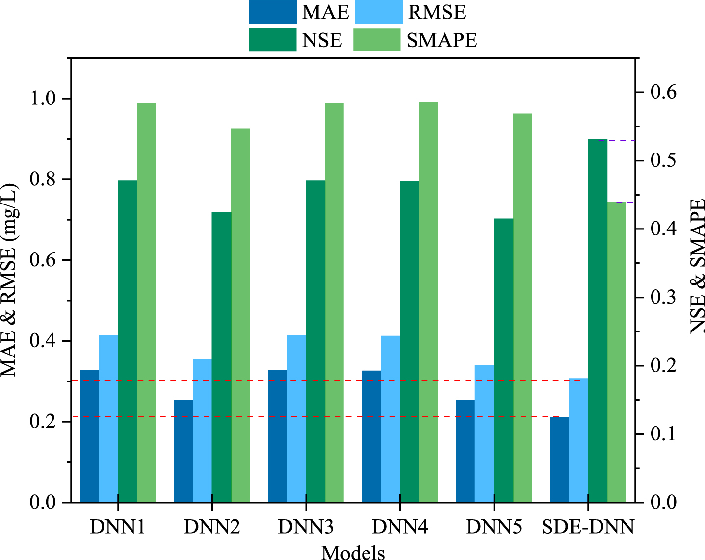
Prediction performance of the proposed SDE-DNN model.

SPSS software is used to analyze the statistical significance of real values and predicted values. Using the paired-sample T test method, the p value is approximately 0.0000, the p value is < 0.01, and the correlation coefficient is 0.7683. Therefore, there is a strong correlation between the two groups of samples; that is, real values and predicted values are highly correlated.

To analyze the influence of the ratio of dividing dataset, test set size is set to 20%, 30%, 40%, 50%, and 60%respectively. The experiment results are shown in Fig. 10. It can be seen that although the MAE and RMSE is the lowest when the test size is 0.3, the NSE is 0.5312 which is the highest and the SMAPE is 0.4392 which is the lowest when test size is 0.4. Therefore, when the test size equals to 0.4, the model’s performance is the best.

Fig. 10

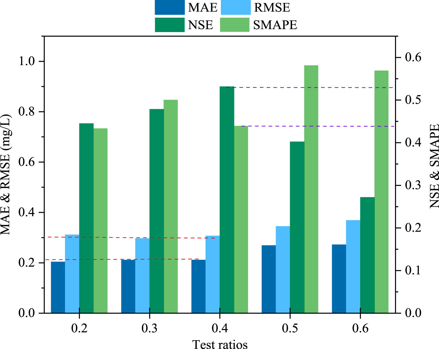
Prediction performance of different ratios.

In order to analyze the water quality prediction of specific lakes, 4 sample points were randomly selected from the data set for experiments with the No. of 14, 66, 112, 258. The number refers to the no. of Table S1 in Appendix A. Figure 11(a) shows the deviation between the observed and predicted values, and Fig. 11(b) shows the absolute error and the absolute error percentage.

Fig. 11

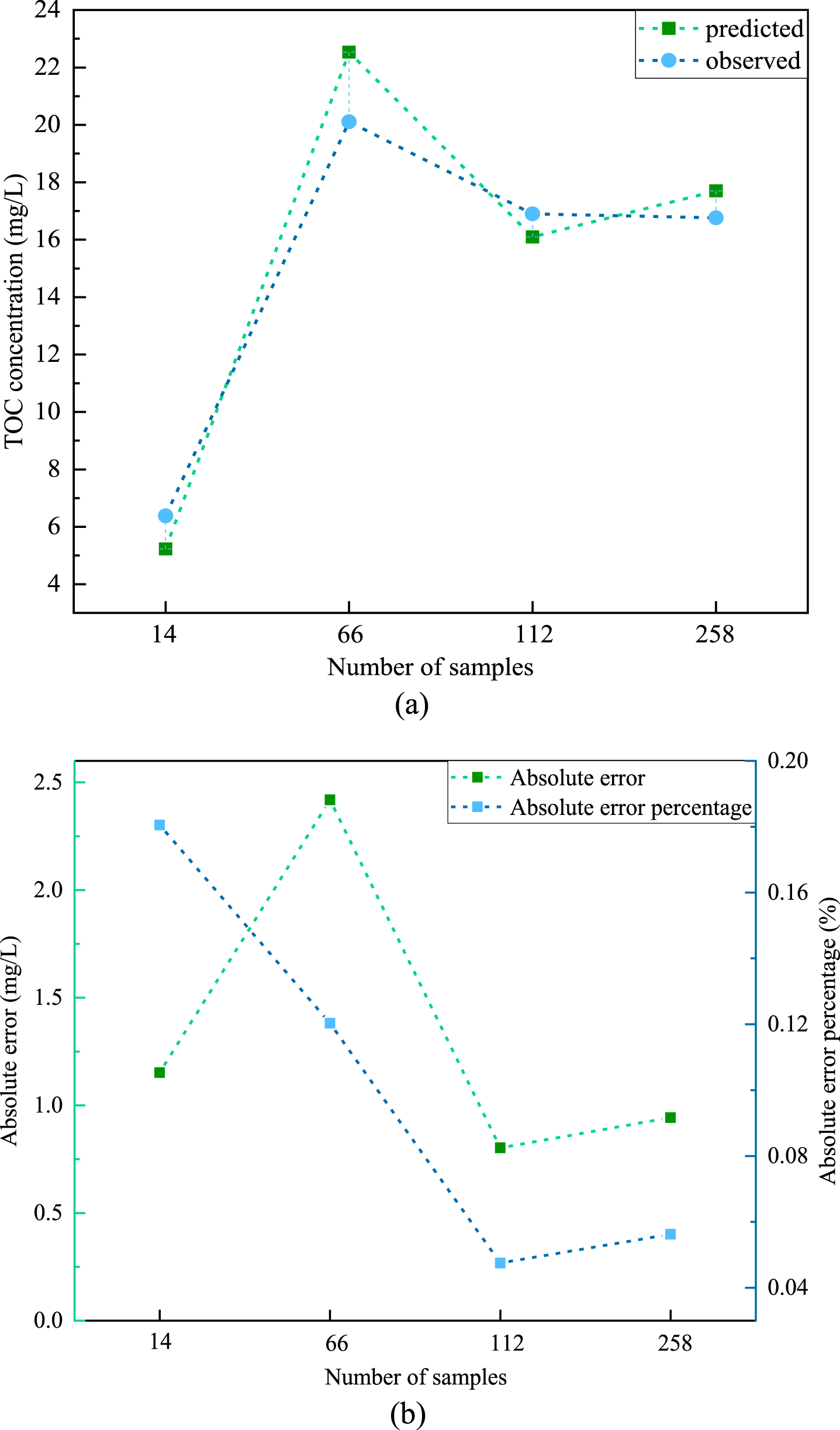
Prediction performance of the specific samples (a) deviation between the observed and predicted values (b) absolute error and absolute error percentage.

Four samples were collected from tph3, dth14, ynh2 and yd2 stations. It can be seen that the percentage of prediction error is generally small, below 20%, while the minimum error percentage of No.112 and No.258 is only 4.74%and 5.62%, that means that the model has a good generalization performance. For No.14, the training data is less, so the prediction error is fairly high. For No.16, although there are many data collected in Dongting Lake, because of the large area of the lake, the uneven development of industry and agriculture and the difference of economic activity around the lake, the prediction error is relatively high, and the absolute error percentage is 12.03%. Overall, the results fully show that the proposed SDE-DNN model has a strong prediction ability for TOC concentration of lakes in the middle and lower reaches of the Yangtze River.

3.6 Compared with other machine learning methods

To verify the effectiveness of the SDE-DNN model in predicting TOC concentration in water, it was compared with other machine learning methods. Selecting the decision tree, linear regression, support vector regression (SVR), K-nearest neighbors (KNN), ridge, lasso and other commonly used machine learning methods, the performance in this sample is shown in Fig. 12. It can be seen that the SVR model performed fairly well in listed above machine learning methods, but it is still poor compared with the proposed SDE-DNN model. Compared with the SDE-DNN model, its MAE is increased by 0.0451 mg/L, and the NSE is decreased by 0.3050.

Fig. 12

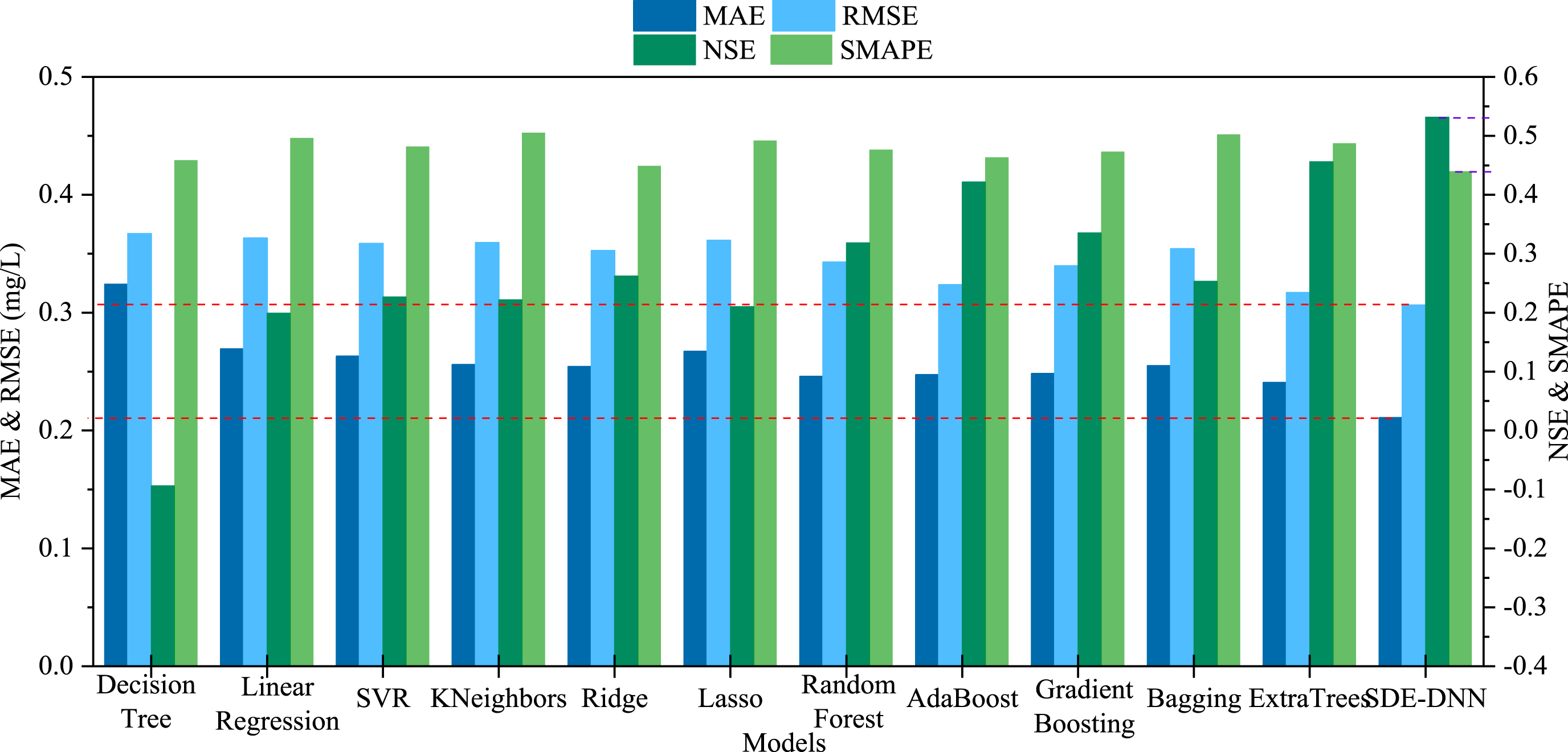
Experiment results of SDE-DNN model and other machine learning models on TOC concentration dataset.

Under the same experimental conditions, the SDE-DNN model is compared with traditional ensemble learning methods such as random forest regression, bagging regression, and AdaBoost regression. After conducting experiments, the results are shown in Fig. 12. It can be seen that the results of ensemble learning method are generally better than those of traditional machine learning methods but still inferior to the proposed SDE-DNN model. Using samples in this paper, the performance of Extra Trees regression method is fairly good, MAE is 0.2406 mg/L, and RMSE is 0.3169 mg/L; however, the result of SDE-DNN is better, with MAE reducing by 0.0298 mg/L and RMSE decreasing by 0.0105 mg/L.

In order to further prove the validity of the model, an additional experiment is conducted on a lake temperature dataset. The dataset is available through a data release on the U.S. Geological Survey’s ScienceBase platform, and all study lakes are located in the Midwestern United States [45]. Figure 13 shows the experiment results. It’s apparently that the SDE-DNN model has a superior prediction performance.

Meanwhile, the Auto MPG data set, PM2.5 data set and kin8 nm data set are selected as common dataset to verify the effectiveness of SDE-DNN. Auto mpg dataset is a slightly modified version of the dataset provided in the StatLib library in 1970 s. In line with the use by Ross Quinlan in predicting the attribute “mpg”. The data concerns city-cycle fuel consumption in miles per gallon, to be predicted in terms of 3 multivalued discrete and 5 continuous attributes [46]. Beijing PM2.5 dataset collected a time period of factors influencing the value of PM2.5 between Jan 1^st, 2010 to Dec 31^st, 2014. It contains 8 attributes to predict the value of PM2.5 [47]. Kin8 nm dataset is concerned with the forward kinematics of an 8 link robot arm. It also contains 8 attributes to predict the target value [48]. Table S3 in the Appendix A presents the results of the experiments. It can be seen that compared with other machine learning models, SDE-DNN has the best regression prediction fitting effect, the highest generalization accuracy and the better universality of the model.

Fig. 13

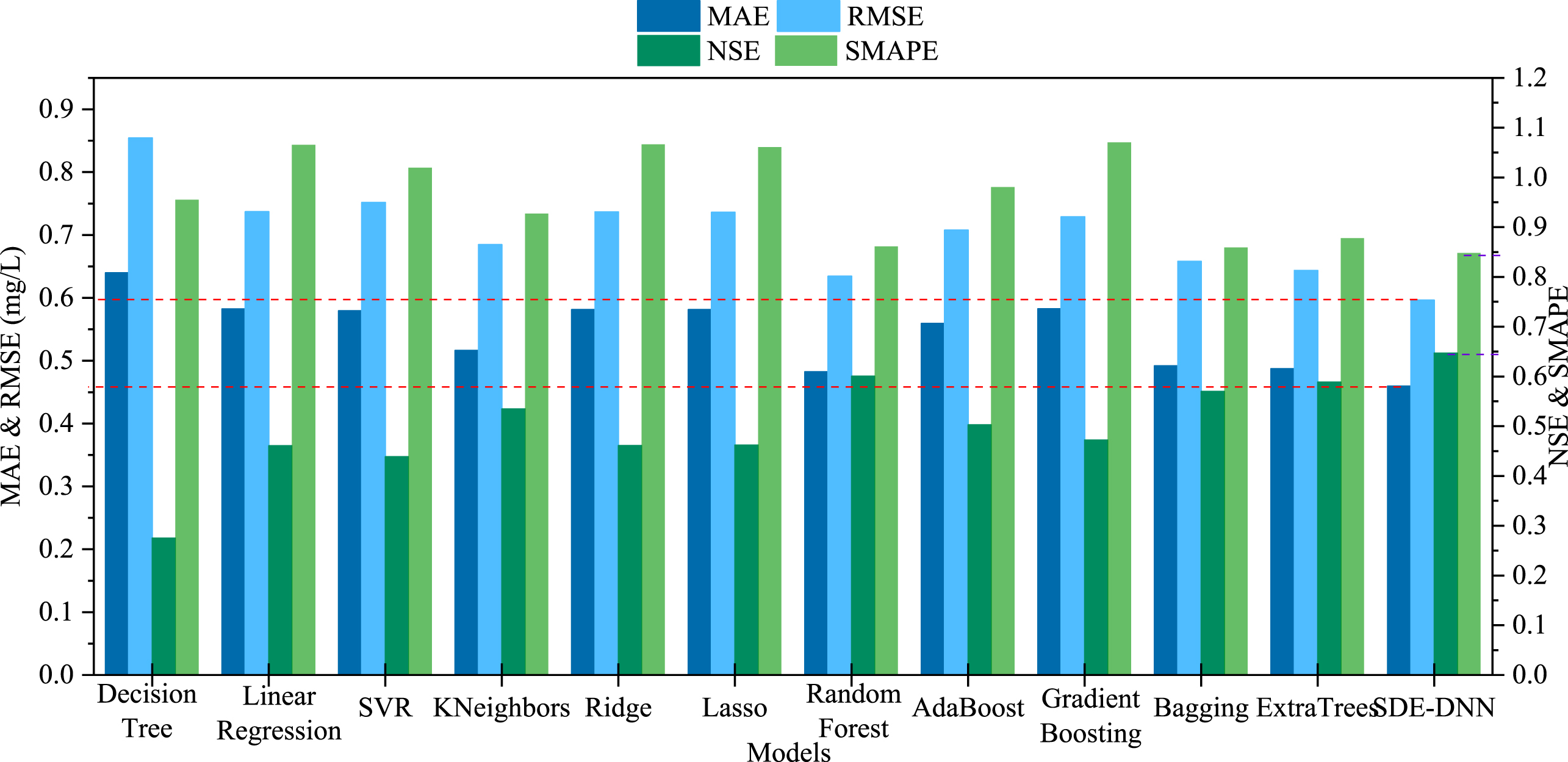
Experiment results of SDE-DNN model and other machine learning models on lake temperature dataset.

4 Discussion

In this paper, the TOC concentration in lakes along the middle and lower reaches of the Yangtze River is studied. Different from the above studied areas, this area is the most densely populated, economically developed and the most frequent industrial production area in China. The lakes area is greatly affected by human activities and industrial production and is vulnerable to pollution, forming a more complex aquatic ecosystem, thus it’s more difficult to predict the TOC concentration. Meanwhile, most of people’s domestic water and agricultural water comes from lakes. Therefore, the requirement for the accuracy of water quality prediction in this area is higher than that in the above study area.

Generally, compared with the shallow learning method such as multiple regression, the deep learning method can extract more information from the data, so as to make more accurate prediction. While the ensemble learning method can improve the prediction performance by combining multiple individual learners.

In this study, a SDE-DNN method is proposed to predict TOC concentration using machine learning method. With 7 water quality parameters as input and the TOC concentration as output, it is feasible to establish a prediction model based on SDE-DNN to predict the concentration of TOC. In order to further verify the effectiveness of the proposed method, SDE-DNN is compared with other TOC prediction methods. These methods come from the literature cited in Introduction. The experiments are conducted on the TOC concentration dataset collected in this paper, and the prediction results are shown in Table 4.

Table 4
Comparison with existing TOC prediction methods

Models RMSE (mg/L) MAE (mg/L) SMAPE NSE

LR [22] 0.3631 0.2691 49.59% 0.1989

LSSVM [24] 0.3907 0.2915 68.45% 0.1757

PLS [21] 0.3279 0.2401 51.38% 0.3201

RF [23] 0.3428 0.2458 47.62% 0.3180

BRNN1 [22] 0.3640 0.2702 48.25% 0.4823

BRNN2 [22] 0.3410 0.2589 49.54% 0.3276

SDE-DNN 0.3064 0.2108 43.92% 0.5312

Models	RMSE (mg/L)	MAE (mg/L)	SMAPE	NSE
LR [22]	0.3631	0.2691	49.59%	0.1989
LSSVM [24]	0.3907	0.2915	68.45%	0.1757
PLS [21]	0.3279	0.2401	51.38%	0.3201
RF [23]	0.3428	0.2458	47.62%	0.3180
BRNN1 [22]	0.3640	0.2702	48.25%	0.4823
BRNN2 [22]	0.3410	0.2589	49.54%	0.3276
SDE-DNN	0.3064	0.2108	43.92%	0.5312

It can be seen that under the same experimental conditions, the prediction error of this model is smaller than that of other existing machine learning models. The result indicates that in lakes along the middle and lower reaches of the Yangtze River, the accuracy of the TOC concentration prediction model based on SDE-DNN is better than other models, and it is more suitable for the prediction of the TOC concentration.

As a universal analysis, the experiments are conducted on the Midwestern United States lake temperature data set. The specific details are shown in section 3.6. The experimental results show that the proposed method is not only suitable for TOC concentration prediction in the middle and lower reaches of the Yangtze River, but also suitable for Midwestern United States lake temperature prediction. Furthermore, experiments are carried out on three common sample sets. The results verify the feasibility and universality of proposed SDE-DNN method.

SDE-DNN method not only has the characteristics of convenience and high prediction accuracy, but also can more accurately analyze the nonlinear relations in complex systems, so as to achieve more accurate real-time prediction of the TOC concentration in lakes under complex nonlinear conditions. It can effectively save funds and time.

However, the research has some limitations. The data collected in this study are concentrated in the drought season, and the attention paid to the water quality data in the rainy season is not enough. Therefore, future research in this area will pay more attention to the balance of data collection, so as to further improve the generalization performance of the model.

With the development of research and application, as an advanced artificial intelligence algorithm and new prediction method, the ensemble learning method will be more widely used in the prediction of the concentration of other substances in water. In the future, more in-depth learning methods can be used to predict the TOC concentration under larger data samples, and the prediction accuracy can be further improved, which can provide more accurate decision-making basis for the sustainable use of water resources.

5 Conclusion

In this paper, an ensemble model namely SDE-DNN is established by stacking five different epochs’ base DNN models in level 0 and a linear regression model in level 1, and applied to predict the TOC concentration in lakes of the middle and lower reaches of the Yangtze River. To verify the effectiveness of the model, 272 pieces of data from the water quality monitoring dataset are selected as samples for experiments. After preprocessing, a dataset with total 379 pieces of data is obtained. Conducting experiments on this dataset. The results show that the model has high prediction precision, MAE is 0.2108 mg/L, SMAPE is 43.92%, NSE is 0.5312, and RMSE is 0.3064 mg/L. The model can well predict the TOC concentration in water. At the same time, the regression accuracy of the SDE-DNN model is better than that of the single DNN model, illustrating that the stacking method can integrate deep neural networks with good effects.

On the water quality monitoring samples of total organic carbon concentration in lakes along the middle and lower reaches of the Yangtze River, the prediction performance of the proposed SDE-DNN model is satisfying. Therefore, using the water quality parameters obtained by sensor networks, the SDE-DNN model can predict the TOC concentration of lakes with high accuracy in real time. The results of this study suggest that the machine learning methods can provide appropriate suggestions on water quality prediction and help for the management of aquatic ecosystems.

However, there are still some deficiencies in this study. The data collected are unbalance, and the prediction results of the proposed model are still unstable, and further experiments are needed to improve its performance. In the future study, on one hand, we will try to increase the samples of each lake of different time and different seasons, and will consider the impact of spatial and geographical location on the water quality of the lake. On the other hand, we will try to change the structure of base DNN model to improve the predicting performance and stability.

Footnotes

Acknowledgments

This work was supported only by the Social Science Fund of Ministry of Education of China (No. 18YJCZH040). Authors gratefully acknowledge the helpful comments and suggestions of the reviewers who improved the presentation.

Appendix A

Table S1

Detailed data of water quality monitoring samples

No.	Date of collection	Station number	Water temperature (°C)	Transparency (m)	pH value	Dissolved oxygen (mg/L)	Conductivity (μs/cm)	Chlorophyll (μg/L)	Ammonia nitrogen (mg/L)	TOC concentration (mg/L)
1	2007/10/11	pyh1	21.44	0.15	7.53	7.15	133.8	3.7	0.1	8.98
2	2007/10/11	pyh2	21.51	0.15	7.73	8.07	133.8	4.67	0.09	8.36
3	2007/10/11	pyh3	21.25	0.1	7.67	8.1	133.8	7	0.12	17.32
4	2007/10/11	pyh4	22.2	0.15	7.72	7.82	133.8	4.33	0.08	8.75
5	2007/10/12	chhu3	21.53	0.8	8.73	9.52	215	6.59	0.09	12.67
6	2007/10/13	pyh5	21.53	0.45	7.89	8.49	93.2	3.6	0.16	8.03
7	2007/10/13	pyh6	21.53	0.3	7.77	7.92	113.5	2.97	0.25	5.97
8	2007/10/13	pyh7	21.53	0.05	7.71	8.64	133.8	9.93	0.23	8.44
9	2007/10/13	pyh8	21.52	0.1	7.72	8.57	133.8	5.67	0.14	9.53
10	2007/10/13	pyh9	21.53	0.05	7.72	8.5	133.8	7.1	0.16	9.41
11	2007/10/13	pyh10	20.57	0.1	7.72	8.53	133.8	8.13	0.13	7.71
12	2007/10/13	pyh11	20.59	0.1	7.65	8.41	133.8	6.1	0.15	7.38
13	2007/10/15	tph1	18.79	0.4	7.9	7.92	174.4	7.74	0.11	5.56
14	2007/10/15	tph2	18.75	0.4	7.98	8.39	174.4	8.23	0.04	6.38
15	2007/10/15	tph3	18.78	0.4	8.14	8.68	174.4	7.33	0.05	6.57
16	2007/10/16	pyh12	19.05	0.1	7.55	8.06	133.8	9.77	0.14	9.36
17	2007/10/16	pyh13	19.15	0.3	7.52	8.08	133.8	5	0.18	8.34
18	2007/10/16	pyh14	19.52	0.3	7.54	8.11	133.8	7.67	0.18	7.71
19	2007/10/16	pyh15	19.31	0.25	7.53	8.25	133.8	3.6	0.2	8.48
20	2007/10/16	pyh16	19.52	0.15	7.56	7.48	133.8	3.9	0.2	9.67
21	2007/10/17	xmh1	18.91	0.3	7.46	8.1	133.8	8.17	0.14	7.98
22	2007/10/17	xmh2	19.05	0.3	7.52	8.11	133.8	8.38	0.15	7.46
23	2007/10/17	xmh3	19.68	0.3	7.96	7.16	133.8	224.19	0.13	7.51
24	2007/10/18	pyh17	19.9	0.2	7.4	7.4	133.8	4.17	0.23	7.61
25	2007/10/18	pyh18	19.49	0.6	7.42	7.55	113.5	2.13	0.19	10.9
26	2007/10/18	pyh19	19.78	0.6	7.48	7.78	113.5	2.42	0.18	7.14
27	2007/10/18	pyh20	19.45	0.5	7.43	7.72	113.5	2.28	0.2	6.6
28	2007/10/18	pyh21	18.8	0.15	7.35	7.4	113.5	5.21	0.15	7.11
29	2007/10/18	pyh22	19.09	0.1	7.39	7.25	133.8	3.47	0.21	7.03
30	2007/10/18	pyh23	19.72	0.25	7.36	7.42	133.8	3.79	0.14	7.35
31	2007/10/18	pyh24	19.41	0.35	7.39	7.64	154.1	3.44	0.32	6.08
32	2007/10/19	nbh1	19.17	0.45	7.64	7.32	215	16.36	0.05	13.37
33	2007/10/19	nbh2	19.3	0.4	8.19	8.5	215	18.5	0.05	12.43
34	2007/10/19	nbh3	19.52	0.4	8.63	9.99	215	19.97	0.04	12.09
35	2007/10/21	bl1	19.78	0.45	8.57	10.15	275.9	21.31	0.04	10.07
36	2007/10/21	sh1	18.83	0.5	8.45	9.17	262.4	5.8	0.04	9.02
37	2007/10/21	sh2	18.86	0.65	8.56	9.3	255.6	4.71	0.04	9.97
38	2007/10/21	sh3	18.85	0.55	8.46	8.48	255.6	6.23	0.04	8.16
39	2007/10/21	sh4	19.17	0.55	8.54	9.4	255.6	4.96	0.05	8.34
40	2007/10/23	zh1	20.1	1.3	8.17	9.16	93.2	2.98	0.03	6.07
41	2007/10/23	zh2	20.25	1.5	7.91	9.01	93.2	2.38	0.04	5.82
42	2007/10/23	zh3	20.22	1.3	7.82	8.54	93.2	3.14	0.04	4.64
43	2007/10/23	zh4	20.23	1.2	7.77	9.18	93.2	2.58	0.03	4.71
44	2007/10/25	jsh2	20.29	1.8	7.29	8.47	72.9	1.28	0.04	4.89
45	2007/10/25	jsh3	20.5	2	7.46	8.44	72.9	1.91	0.05	5.83
46	2007/10/25	jsh4	20.81	1.5	7.78	8.17	72.9	2.49	0.04	6.1
47	2007/10/25	jsh5	20.5	1.5	7.1	8.3	72.9	1.68	0.04	5.79
48	2007/10/25	jsh6	20.6	1.5	7.21	8.4	72.9	1.91	0.09	6.1
49	2007/10/25	jsh7	20.15	1.5	7.27	8.55	72.9	1.33	0.04	4.68
50	2007/10/26	cj1	19.78	0.3	7.12	7.35	93.2	8.83	0.11	5.88
51	2007/10/26	cj2	20.31	0.3	6.89	7.59	93.2	7.38	0.05	5.39
52	2007/10/26	cj3	20.77	0.3	7.03	7.68	93.2	7.06	0.06	5.63
53	2007/11/1	dth1	16.73	0.3	8.16	8.02	215	1.52	0.15	24.67
54	2007/11/1	dth2	17.06	0.7	8.18	8.22	235.3	1.07	0.15	25.46
55	2007/11/1	dth3	17.06	0.6	8.19	7.96	215	1.73	0.15	21.72
56	2007/11/1	dth4	16.99	0.4	8.18	7.88	215	2.36	0.15	21.19
57	2007/11/1	dth5	16.83	0.6	8.15	7.96	215	1.74	0.15	22.47
58	2007/11/1	dth6	16.97	0.5	8.22	7.66	215	1.28	0.15	24.71
59	2007/11/1	dth7	16.91	0.45	8.47	7.87	235.3	2.6	0.17	27.65
60	2007/11/2	dth8	18.68	0.8	7.98	7.47	215	1.5	0.23	25.64
61	2007/11/2	dth9	18.37	0.7	8.11	7.75	215	0.91	0.13	22.94
62	2007/11/2	dth10	18.47	0.7	8.08	7.89	215	1.49	0.13	22.02
63	2007/11/2	dth11	18.17	0.7	8.07	7.56	215	1.32	0.11	22.97
64	2007/11/2	dth12	17.83	0.9	8.08	7.83	215	1.13	0.15	27.44
65	2007/11/2	dth13	17.72	0.9	8.13	7.8	215	1.18	0.13	21.69
66	2007/11/2	dth14	17.71	0.8	8.13	8.41	215	1.63	0.12	20.11
67	2007/11/3	dth1-2	14.9	0.6	7.94	4.4	174.4	3.69	0.33	6.36
68	2007/11/3	dth2-2	15.72	1.1	7.88	9.05	133.8	1.87	0.26	12.63
69	2007/11/3	dth3-2	15.67	0.5	7.67	6.24	160.9	5.53	0.19	16.19
70	2007/11/5	hndh1	16.03	0.65	7.95	8.74	316.5	7.07	0.37	15.05
71	2007/11/5	hndh2	15.65	0.25	7.88	7.96	316.5	9.16	0.53	14.6
72	2007/11/5	hndh3	16	1.2	8.35	9.71	316.5	9.03	0.38	15.45
73	2007/11/6	dath1	14.76	0.6	8.16	8.33	336.8	2.55	0.32	31.82
74	2007/11/6	dath2	14.89	0.5	8.13	8.4	336.8	3.4	0.43	28.38
75	2007/11/6	dath3	15.1	0.4	8.35	8.79	357.1	10.57	0.29	31.9
76	2007/11/6	dath4	15.25	0.4	8.15	8.63	336.8	2.3	0.22	29.06
77	2007/11/6	dath5	15.11	0.5	8.41	9.3	336.8	5.32	0.29	27.63
78	2007/11/6	dath6	15.53	0.3	8.32	8.84	336.8	6.25	0.14	28.16
79	2007/11/7	dth15	15.32	0.5	8.02	7.64	357.1	2.53	0.08	32.48
80	2007/11/10	lyh1	16.83	0.3	8.13	8	235.3	5.23	0.19	19.02
81	2007/11/10	lyh2	16.82	0.6	8.02	7.95	215	4.78	0.22	18.85
82	2007/11/10	lyh3	17.23	0.6	8.28	9.36	215	8.72	0.23	17.38
83	2007/11/11	mlh1	16.57	0.6	7.91	8.88	154.1	13.22	0.15	35.51
84	2007/11/11	mlh2	16.85	0.8	8.32	9.51	174.4	10.48	0.2	29.15
85	2007/11/11	mlh3	16.49	0.4	7.71	8.55	154.1	11.59	0.21	36.03
86	2007/11/11	shanbh1	15.58	0.4	8.75	8.7	397.7	16.92	0.21	9.52
87	2007/11/11	shanbh2	15.84	0.6	8.44	8.31	397.7	14.48	0.11	9.98
88	2007/11/11	shanbh3	15.84	0.5	8.46	7.73	397.7	13.47	0.12	9.1
89	2007/11/12	bem1	15.13	0.25	8.02	8.39	248.8	11.81	0.28	12.42
90	2007/11/12	bem2	15.12	0.5	7.81	8.48	255.6	15.57	0.3	11.38
91	2007/11/19	dth16	14.01	0.25	8.26	8.5	296.2	4.14	0.11	20.07
92	2007/11/19	dth17	14.64	0.3	8.09	7.89	275.9	2.9	0.33	22.97
93	2007/11/19	dth18	14.71	0.25	8.08	7.89	275.9	2.59	0.39	22.16
94	2007/11/19	dth20	14.67	0.25	8.09	8.06	275.9	3.2	0.35	17.96
95	2007/11/19	dth21	14.87	0.2	8.12	8	275.9	2.14	0.34	22.75
96	2007/11/19	dth22	14.74	0.25	8.11	8.04	275.9	2.94	0.34	21.09
97	2007/11/19	dth23	14.97	0.3	8.12	8.04	275.9	2.5	0.33	20.92
98	2007/11/20	nh1	14.23	0.9	8.28	7.89	316.5	13.93	0.27	24.83
99	2007/11/20	nh2	14.39	0.6	8.01	6.13	316.5	13.99	0.16	25.9
100	2007/11/21	bj2	17.33	0.35	8.7	8.96	275.9	16.18	0.1	27.25
101	2007/11/22	hugh1	13.48	0.25	8.53	10.23	255.6	23.87	0.22	31.15
102	2007/11/22	hugh2	12.97	0.5	8.71	11.77	316.5	18.33	0.75	32.77
103	2008/3/5	chah1	11.6	1.3	8.55	13.2	279	8.2	0.01	13.32
104	2008/3/5	chah2	11.35	1.55	8.57	13	282.7	7.7	0.48	12.69
105	2008/3/5	chah3	11.3	1.45	8.64	14.6	287	11.2	0.37	17.2
106	2008/3/6	chah4	11.33	1	8.47	12.2	329	13.6	0.03	15.85
107	2008/3/6	chah5	11.61	1.2	8.34	10.5	373.7	15.7	0.05	15.24
108	2008/3/6	chah6	11.77	0.5	8.47	11.8	392	24.5	0.82	21.51
109	2008/3/7	chh1	9.13	0.2	8.43	9.6	367	4.7	0.04	28.9
110	2008/3/7	chh2	9.27	0.2	8.32	10	362	5.2	0.04	18.58
111	2008/3/7	ynh1	11.22	0.5	8.12	9.7	225	14.2	0.07	14.82
112	2008/3/7	ynh2	11.06	0.5	8.12	9.9	233	11.9	0.08	16.9
113	2008/3/8	nlh1	10.76	0.85	8.13	10	210.3	2	0.03	11.04
114	2008/3/8	nlh2	11	0.9	7.92	10.2	208	1.5	0.03	12.77
115	2008/3/8	yh1	11.92	0.2	8.4	10.2	364	8	0.14	40.28
116	2008/3/9	shajh1	11.82	0.85	8.17	9.7	288	3.9	0.03	16.81
117	2008/3/9	shajh2	12.26	0.8	8.08	9.4	283.7	5.1	0.02	13.76
118	2008/3/10	hh3	14.48	0.4	8.52	10.7	303.3	4.4	0.02	16
119	2008/3/10	hh4	15.13	0.6	8.49	10.8	294.7	6.4	0.03	22.7
120	2008/3/10	hh6	16.06	0.6	8.5	9.5	271.5	2.7	0.02	16.6
121	2008/3/12	hbdh1	16.4	0.4	9.15	17	332.3	29.4	0.02	14.13
122	2008/3/12	hbdh2	14.86	0.4	8.81	13.1	320.5	16.7	0.03	19.9
123	2008/3/12	hbdh3	4.7	0.5	8.57	10.8	350	6.8	0.04	20.5
124	2008/3/14	tjh1	14.7	0.1	8.02	7.4	245	1.6	0.1	14.44
125	2008/3/14	tjh2	15.64	0.1	7.92	8.8	263	6.5	0.02	11.76
126	2008/3/14	yzh1	17.22	1	9.97	13.1	276.7	3.8	0.03	21.71
127	2008/3/14	yzh2	17.1	0.6	9.7	12.3	321	19.4	0.04	18.09
128	2008/3/14	yzh3	16.72	0.35	9.14	10.5	367	12.8	0.94	25.14
129	2008/3/15	hbnh1	18.75	0.3	8.85	11	359.5	25.1	0.04	16.32
130	2008/3/15	hbnh1	21.25	0.4	9.05	13.4	351	32.3	0.02	15.67
131	2008/3/17	dxch3	17.05	0.65	9.59	12.6	383	9.4	0.04	11.25
132	2008/3/19	wh1	18.53	1	8.38	10.9	216	3.2	0.02	10.33
133	2008/3/19	wh2	18.22	1.2	8.57	10.7	212	6.4	0.03	10.08
134	2008/3/19	zdh1	16.45	0.5	8.47	10	295	21.5	0.03	13.77
135	2008/3/19	zdh2	15.88	0.4	8.49	9.7	298	22.3	0.02	19.71
136	2008/3/19	zdh3	16.29	0.65	8.53	10	297	14.8	0.02	17.39
137	2008/3/20	lh1	17.41	0.55	8.64	10.3	206	4.8	0.03	14.09
138	2008/3/20	lh2	17.91	0.3	8.29	9.7	244	9.6	0.02	11.55
139	2008/3/20	lh3	18.53	0.35	8.3	9.8	253	6.9	0.01	21.27
140	2008/3/21	xlh3	16.95	0.65	8.14	9.2	204	14.3	0.36	14.75
141	2008/3/22	fth1	13.62	0.4	8.46	10.2	206	7.5	0.04	23.41
142	2008/3/22	fth3	17.07	0.35	9.5	14.8	158	3.9	0.14	17.67
143	2008/3/23	ssh1	17.24	0.45	8.52	10.9	202	3.2	0.05	11.3
144	2008/3/24	hyxh1	16.5	1.6	8.49	9.5	263	3.6	0.24	14.93
145	2008/3/24	hyxh2	16.92	1.5	8.72	11.4	260	4.2	0.03	12.13
146	2008/3/24	hgh1	18.98	1.5	9.27	12.4	251.3	8.1	0.05	25.16
147	2008/3/24	hgh2	19.25	0.6	8.97	12.5	294.7	24.9	0.23	13.32
148	2008/3/26	txh1	17.05	0.7	8.73	10.8	370.3	16	0.37	18.4
149	2008/3/26	txh2	17.24	0.7	9.25	13.6	388.8	40.6	0.08	29.8
150	2008/3/26	txh3	17.51	0.6	9.08	12.2	378	30.8	0.13	28.53
151	2008/3/27	yxh1	18.03	0.75	8.71	10.7	367.3	17.4	0.16	18.67
152	2008/3/27	yxh2	18.59	0.6	8.86	11.8	383.3	22.3	0.12	30.14
153	2008/3/28	lzh1	17.77	3	8.05	9.1	157	3	0.03	15.35
154	2008/3/28	lzh2	17.95	3	8.16	9.1	168	3.2	0.02	17.15
155	2008/3/28	lzh4	17.14	2.4	8.56	9.8	165.3	1.2	0.03	18.58
156	2008/3/29	lzh5	16.39	2.5	9.11	10.7	151	3.9	0.03	20.24
157	2008/3/29	lzh6	16.3	2.2	8.96	10	170	3.6	0.04	22.4
158	2008/3/29	lzh7	16.45	0.8	8.29	9.1	209	2.9	0.02	20.44
159	2008/3/30	ba1	14.26	1	8.48	9.6	407.7	2.8	0.04	17.33
160	2008/3/30	ba2	14.62	0.75	8.36	9.8	448.7	5.4	0.02	16.53
161	2008/3/30	ba3	14.55	1	8.1	10.2	628	5.2	0.02	15.11
162	2008/3/30	sash1	13.52	0.7	8.4	10.6	232.5	4.5	0.38	25.9
163	2008/3/30	sash2	14.07	0.5	8.51	10.5	408.5	8.2	0.01	26.52
164	2008/3/31	hush1	13.13	0.4	9.25	11.4	250	4.7	0.14	15.35
165	2008/3/31	hush2	12.96	0.5	9.76	10.4	239	2.5	0.01	19.42
166	2008/4/1	ceh1	12.98	0.3	9.71	10.4	159	3.2	0.05	25.66
167	2008/4/1	ceh2	13.12	0.3	10	11.8	147.5	5.8	0.01	20.32
168	2008/4/1	cd1	14.4	0.2	8.84	12.1	253.5	46.6	0.01	23.27
169	2008/4/1	cd2	14.65	0.25	8.46	9.6	215	12.6	0.03	24.06
170	2008/4/1	cd3	14.86	0.25	8.63	10.3	251.7	33.4	0.02	26.05
171	2008/4/2	wah1	14.74	0.45	8.62	10.4	226.7	10.1	0.3	28.62
172	2008/4/2	wah2	14.46	0.6	8.65	10.5	226	8.1	0.05	21.73
173	2008/4/2	wah3	14.74	0.9	8.54	10	227.7	5.4	0.01	27.2
174	2008/4/2	zph1	13.1	0.8	8.44	8.7	338.5	6.6	0.22	26.78
175	2008/4/2	zph2	13.06	0.7	8.36	8.6	324	6.7	0.76	27.87
176	2008/4/3	dyh1	16.54	0.35	8.16	7.5	705	3.7	0	30.43
177	2008/4/3	dyh2	16.32	0.6	8.57	11.4	556.5	7.8	0.02	13.9
178	2008/4/3	dyh3	15.37	0.45	8.4	10	578.5	15.2	0.21	27.81
179	2008/4/4	wsh1	14.78	0.4	8.55	11.1	409.5	58.4	0.98	37.46
180	2008/4/4	wsh2	14.72	0.3	8.29	9	460.5	52.2	0.89	26.66
181	2008/4/5	tbh1	15.64	0.5	8.9	10.9	245	27	0.27	18.07
182	2008/4/5	tbh2	15.34	0.6	8.92	11.3	284.5	21.9	0.35	21.09
183	2008/4/5	tbh3	15.44	0.6	9.04	13.2	379	39.8	0.63	21.84
184	2008/4/6	lgh2	17.99	0.4	8.77	10.2	356	10.1	0.49	27.73
185	2008/4/6	lgh3	19.78	0.4	8.5	10.2	244	8.2	0.02	20.78
186	2008/4/6	lgh4	16.99	0.8	9.48	10.2	232	3.9	0.22	17.02
187	2008/4/7	lgh5	21.09	0.4	8.62	9.4	346	2.6	0.28	25.58
188	2008/4/7	lgh6	21.14	0.4	8.97	10	313	5.1	0.62	33.47
189	2008/4/7	lgh7	21.26	0.5	9.33	11.3	248	7	1.18	24
190	2008/4/7	lgh8	22.33	0.25	8.63	9.4	211	11.3	0.2	21.29
191	2008/4/8	hdh1	22.33	0.45	9.51	9.7	282	12.5	0.4	17.24
192	2008/4/8	hdh2	21.33	0.45	9.19	8.7	301	7.8	0.44	18.43
193	2008/4/8	hdh4	21.99	0.4	8.97	8.5	295	8.1	0.1	18.79
194	2008/4/9	hdh5	19.1	0.05	8.26	8.3	278	25.9	0.2	23.19
195	2008/4/10	bh1	19.15	0.05	8.24	8.8	168	11.7	0.04	20.76
196	2008/4/10	bh2	18.62	0.2	8.56	9.3	153	5.9	0.24	20.32
197	2008/4/10	bh3	18.66	0.2	8.4	9.3	144	12.7	0.35	11.61
198	2008/4/10	bh4	18.68	0.35	8.86	9.8	214	4	0.19	18.65
199	2008/4/10	bh5	18.75	0.35	8.8	9.9	207	6	0.31	24.82
200	2008/4/11	wch1-2	17.47	0.25	8.31	8.9	132	8.9	0.03	12.53
201	2008/4/11	wch2-2	17.63	0.3	8.03	8.5	129	7.6	0.19	9.04
202	2008/4/15	shjh1	16.16	0.35	8.33	8.6	193	5	0.06	21.43
203	2008/4/15	shjh2	16.14	0.25	8.44	8.9	183	11.7	0.04	21.73
204	2008/4/16	pgh1	16.59	0.5	8.9	10	250	9.8	0.03	24.88
205	2008/4/16	pgh2	16.16	0.5	8.48	9.3	264	10.8	0.03	33.3
206	2008/4/17	bd1	22.32	0.3	8.53	9.9	207	1.8	0.05	10.89
207	2008/4/17	cz1-2	16.54	0.2	8.02	7.7	175	5.5	0.14	18.2
208	2008/4/17	cz2-2	14.38	0.1	8.57	7.8	188	5.1	0.17	23.19
209	2008/10/25	dzh1	17.6	0.4	7.9	5.76	566	3.2	0.27	39.04
210	2008/10/25	dzh2	17.97	0.45	8.09	7.73	621	6.5	0.14	31.4
211	2008/11/21	cha1	11.94	0.3	8.57	11.43	292	6.4	0.25	20.46
212	2008/11/21	cha2	11.92	0.3	8.43	10.45	281	7.5	0.06	19.97
213	2008/11/21	cha3	11.87	0.25	8.39	10.3	289	5.9	0.05	19.18
214	2008/11/21	cha4	12.22	0.25	8.35	11.26	285	6	0.05	19.55
215	2008/11/21	cha5	12.31	0.3	8.38	10.88	291	5.2	0.04	20.01
216	2008/11/21	cha6	12.33	0.5	8.36	11.57	308	4.8	0.07	19.77
217	2008/11/21	cha7	12.31	0.3	8.34	10.49	292	5.6	0.06	19.24
218	2008/11/21	cha8	12.39	0.35	8.38	9.51	301	6.3	0.09	19.13
219	2008/11/21	cha9	11.8	0.2	8.35	10.99	274	4.3	0.27	17.74
220	2008/11/21	cha10	11.55	0.2	8.15	9.98	290	5.4	0.04	22.48
221	2008/11/21	cha11	11.76	0.2	8.21	10.13	296	5.6	0.15	19.86
222	2008/11/21	cha12	12.04	0.2	8.16	9.99	328	7.2	0.38	24.06
223	2008/11/21	cha13	11.97	0.2	8.13	10.18	258	3.9	0.27	15.25
224	2009/3/26	gch1	12.76	0.45	8.23	10.68	320	8.5	0.59	22.74
225	2009/3/26	gch2	12.47	1	8.29	10.67	323	3.6	0.33	22.3
226	2009/3/26	gch3	12.7	0.25	8.22	10.51	329	6.1	0.31	19.01
227	2009/3/26	gch4	13.01	2.2	8.26	10.78	366	1.9	0.27	19.81
228	2009/3/27	nyh1	11.78	0.45	8.22	10.69	214	5.8	0.58	8.6
229	2009/3/27	nyh2	11.92	0.75	8.11	10.57	186	9.9	0.81	9.84
230	2009/3/27	nyh3	11.75	0.25	8.09	10.79	139	4.4	0.21	11.52
231	2009/3/27	nyh4	11.74	0.3	8.04	10.6	119	3	0.21	6.58
232	2009/3/27	nyh5	11.95	0.2	7.98	10.7	140	6.4	0.1	5.19
233	2009/3/27	nyh6	11.67	0.55	7.72	11.01	188	10	0.3	7.08
234	2009/3/27	sjh2	13.05	0.3	8.3	10.68	267	11.9	0.07	17.36
235	2009/3/27	sjh3	13.03	0.2	8.37	10.37	251	20.1	0.09	13.79
236	2009/3/27	sjh7	13.2	0.75	8.23	10.43	300	12.5	0.14	18.6
237	2009/3/30	sjh1	11.12	0.25	8.48	11.34	251	13.1	0.07	16.32
238	2009/3/30	sjh4	10.97	0.75	8.3	11.36	289	9.1	0.14	17.75
239	2009/3/30	sjh5	11.24	1	8.44	11.48	339	5.1	0.13	13.02
240	2009/4/1	gh1	12.22	0.3	8.22	10.48	569	15.5	2.45	16.79
241	2009/4/1	gh2	12.02	0.3	8.31	10.82	596	21.2	1.46	16.85
242	2009/4/1	gh3	12.97	0.25	8.22	10.36	647	22.1	2.27	27.01
243	2009/4/1	gh4	12.84	0.25	8.76	11.34	572	42.6	0.63	20.1
244	2009/4/1	gh5	12.86	0.3	8.78	12.27	628	30.9	1.06	17.8
245	2009/4/1	gh6	12	0.3	8.27	10.33	605	21.8	0.91	18.99
246	2009/4/2	cdh1	12.21	0.5	8.64	10.98	543	13.5	0.55	13.69
247	2009/4/2	cdh2	11.81	0.3	8.56	11.27	700	26.1	1.42	17.93
248	2009/4/2	cdh3	11.39	0.25	8.54	11.34	601	24.7	0.99	17.02
249	2009/4/2	cdh4	11.85	0.35	8.75	11.52	640	25	0.7	23.64
250	2009/4/2	cdh5	12.08	0.4	8.4	10.65	592	12.6	1.3	17.06
251	2009/4/3	xzdq1	12.25	0.25	8.25	10.52	598	15.1	1.95	17.42
252	2009/4/3	xzdq2	13.16	0.35	8.51	11.19	562	34	1.25	21.25
253	2009/4/3	xzdq3	12.6	0.35	8.3	10.8	595	20.9	1.44	19.92
254	2009/4/5	dsh1	13.95	0.5	8.26	10.62	695	7.2	0.26	18.08
255	2009/4/5	dsh2	13.96	0.45	8.22	10.14	739	14.5	2.25	14.71
256	2009/4/5	dsh3	13.76	0.4	8.53	11.39	860	17.7	0.45	18.6
257	2009/4/5	dsh4	14.07	0.5	8.45	11.08	789	15.5	0.36	21.94
258	2009/4/5	yd2	14.4	1	8.06	40.08	691	7.3	0.37	16.76
259	2009/4/6	ch1	15.61	0.5	8.13	10.29	768	16.6	2.69	13.16
260	2009/4/6	ch2	5.49	0.6	8.51	10.63	778	24	2.02	12.47
261	2009/4/6	ch3	15.64	0.65	8.58	10.78	774	24.5	0.79	12.55
262	2009/4/7	kch1	13.98	0.7	8.39	10.02	900	18.4	0.8	19.86
263	2009/4/7	kch2	14.61	0.9	8.49	11.47	935	26.5	0.77	21.76
264	2009/4/7	kch3	15.1	0.9	8.73	11.3	907	25.6	0.39	18.14
265	2009/4/9	ych1	16.93	1.1	8.94	11.86	822	23.4	1.03	13.86
266	2009/4/9	ych2	17.83	0.9	9.05	12.98	763	21.5	0.11	13.79
267	2009/4/9	ych3	16.61	0.8	8.88	11.72	849	20.6	0.08	23.74
268	2009/4/9	ych4	18.09	0.8	9.04	12.65	780	15.4	0.92	29.88
269	2009/4/9	ych5	16.31	0.7	8.69	11.28	849	8.2	0.15	23.07
270	2009/4/9	ych6	16.56	0.9	8.5	10.41	838	7	0.19	21.84
271	2009/4/9	ych7	17.43	1	9.03	13.12	768	34.2	0.35	20.83
272	2009/4/9	ych8	18.14	1	9.05	13.04	759	12.9	0.1	17.9

Table S2

Table of lake stations and names

Stations	Name of lakes	Number of samples
bl	Bali Lake	1
bj	Bajiao Lake	1
bd	Baidang Lake	1
ba	Bao’an Lake	3
bem	Beimin Lake	2
bh	Bo Lake	5
cz	Caizi Lake	2
ceh	Ce Lake	2
cha	Chao Lake	13
cj	Chenjia Lake	3
ch	Cheng Lake	3
cd	Chidong Lake	3
chhu	Chi Lake	1
chh	Chong Lake	2
dath	Datong Lake	6
dyh	Daye Lake	3
dzh	Dazong Lake	2
dsh	Dingshan Lake	4
hndh	Dong Lake (Hunan)	3
hbdh	Dong Lake (Hubei)	3
dxch	Dongxicha Lake	1
dth	Dongting Lake	25
fth	Futou Lake	2
gh	Ge Lake	6
gch	Gucheng Lake	4
hyxh	Hanyangxi Lake	2
hh	Hong Lake	3
hgh	Houguan Lake	2
hdh	Huangda Lake	4
hugh	Huanggai Lake	2
hush	Huangshan Lake	2
jsh	Junshan Lake	6
kch	Kuncheng Lake	3
lzh	Liangzi Lake	6
lyh	Liuye Lake	3
lgh	Longgan Lake	7
lh	Lu Lake	3
mlh	Maoli Lake	3
nbh	Nanbei Lake	3
nh	Nan Lake (Hunan)	2
hbnh	Nan Lake (Hubei)	2
nyh	Nanyi Lake	6
nlh	Niulang Lake	2
pyh	Poyang Lake	24
pgh	Pogang Lake	2
sh	Sai Lake	4
sash	Sanshan Lake	2
shanbh	Shanpo Lake	3
shajh	Shangjin Lake	2
ssh	ShangShe Lake	1
shjh	Shengjin Lake	2
sjh	Shijiu Lake	6
tbh	Taibai Lake	3
tph	Taibo Lake	3
txh	Tangxun Lake	3
tjh	Tongjia Lake	2
wah	Wang Lake	3
wch	Wuchang Lake	2
wh	Wu Lake	2
wsh	Wushan Lake	2
xzdq	Xiqiu Lake, Zhongqiu Lake, Dongqiu Lake	3
xlh	Xiliang Lake	1
xmh	Xinmiao Lake	3
yxh	Yanxi Lake	2
ych	Yangcheng Lake	8
yzh	Yezhu Lake	3
ynh	Yuni Lake	2
yh	Yu Lake	1
yd	Yuandang Lake	1
cdh	Changdang Lake	5
chah	Chang Lake	6
zdh	Zhangdu Lake	3
zph	Zhupo Lake	2
zh	Zhu Lake	4

Table S3

Prediction results of SDE-DNN and other machine learning methods on different datasets

Dataset	Methods	RMSE	MAE	SMAPE	NSE
Auto MPG	DecisionTree	0.2132	0.1504	60.5222%	0.7314
	LinearRegression	0.1727	0.1337	58.6079%	0.8238
	SVR	0.1443	0.1113	52.1369%	0.8770
	KNeighbors	0.1649	0.1217	55.0764%	0.8393
	Ridge	0.1728	0.1338	58.7938%	0.8237
	Lasso	0.2786	0.2249	94.9539%	0.5414
	RandomForest	0.1433	0.1046	48.1114%	0.8787
	AdaBoost	0.1667	0.1262	56.0834%	0.8358
	GradientBoost	0.1549	0.1138	50.5540%	0.8582
	Bagging	0.1424	0.1057	48.4316%	0.8802
	ExtraTrees	0.1393	0.1020	46.5672%	0.8853
	SDE-DNN	0.1329	0.1010	48.7495%	0.8957
PM2.5	DecisionTree	0.1154	0.0588	13.7670%	0.8793
	LinearRegression	0.1388	0.0821	19.8851%	0.8252
	SVR	0.0877	0.0598	13.2228%	0.9302
	KNeighbors	0.0969	0.0533	12.7350%	0.9149
	Ridge	0.1388	0.0821	19.8625%	0.8252
	Lasso	0.3198	0.2366	36.7665%	0.0724
	RandomForest	0.0947	0.0469	11.4596%	0.9186
	AdaBoost	0.1130	0.0812	16.8880%	0.8843
	GradientBoost	0.0911	0.0526	12.7182%	0.9247
	Bagging	0.0935	0.0466	11.2628%	0.9207
	ExtraTrees	0.0787	0.0428	10.6588%	0.9438
	SDE-DNN	0.0722	0.0425	10.8739%	0.9526
Kin8nm	DecisionTree	0.3262	0.2497	101.4621%	0.2221
	LinearRegression	0.2835	0.2284	108.3427%	0.4125
	SVR	0.1166	0.0898	53.1576%	0.9006
	KNeighbors	0.1834	0.1428	75.1948%	0.7540
	Ridge	0.2835	0.2284	108.3448%	0.4125
	Lasso	0.3593	0.2935	156.7537%	0.0558
	RandomForest	0.2149	0.1703	86.6000%	0.6623
	AdaBoost	0.2960	0.2464	113.6831%	0.3595
	GradientBoost	0.2606	0.2093	101.8058%	0.5034
	Bagging	0.2161	0.1716	87.5931%	0.6584
	ExtraTrees	0.2079	0.1659	85.5067%	0.6841
	SDE-DNN	0.0990	0.0771	47.3453%	0.9283

References

Lei

, et al., Water remote sensing eutrophication inversion algorithm based on multilayer convolutional neural network, Journal of Intelligent & Fuzzy Systems 39(4) (2020), 5319–5327.

Wang

W.W.

, Zhou

H.W.

and Guo

L.D.

, Emergency water supply decision-making of transboundary river basin considering government–public perceived satisfaction, Journal of Intelligent & Fuzzy Systems 40(1) (2021), 381–401.

Hernandez-Ramirez

A.G.

, Martinez-Tavera

, Rodriguez-Espinosa

P.F.

, et al., Detection, provenance and associated environmental risks of water quality pollutants during anomaly events in River Atoyac, Central Mexico: A real-time monitoring approach, Science of the Total Environment 669 (2019), 1019–1032.

Mwaijengo

G.N.

, Msigwa

, Njau

K.N.

, et al., Where does land use matter most? Contrasting land use effects on river quality at different spatial scales, Science of the Total Environment 715 (2020), 134825.

S.M.

, Marinaite

I.I.

, Zhuchenko

N.A.

, et al., Revealing the factors affecting occurrence and distribution of polycyclic aromatic hydrocarbons in water and sediments of Lake Baikal and its tributaries, Chemistry and Ecology 34(10) (2018), 1–16.

, Li

, et al., Comparison of Prokaryotic Communities Associated with Different TOC Concentrations in Dianchi, Water 12(9) (2020), 2557.

Yan

, Microbial control of river pollution during covid-19 pandemic based on big data analysis, Journal of Intelligent & Fuzzy Systems 39(6) (2020), 8937–8942.

Fiskal

, Deng

, Michel

, et al., Effects of eutrophication on sedimentary organic carbon cycling in five temperate lakes, Biogeosciences 16(19) (2019), 3725–3746.

Engel

, Drakare

and Weyhenmeyer

G.A.

, Environmental conditions for phytoplankton influenced carbon dynamics in boreal lakes, Aquatic Sciences 81(2) (2019), 35–47.

10.

Sousa

, Ribeiro

, Barbosa

, Pereira

and Silva

, A review on environmental monitoring of water organic pollutants identified by EU guidelines, Journal of Hazardous Materials 344 (2018), 146–162.

11.

Feld

C.K.

, Saeedghalati

and Hering

, A framework to diagnose the causes of river ecosystem deterioration using biological symptoms, Journal of Applied Ecology 57(11) (2020), 2271–2284.

12.

Din

E.S.E.

, A novel approach for surface water quality modelling based on Landsat-8 tasselled cap transformation, International Journal of Remote Sensing 41(18) (2020), 7186–7201.

13.

Carminati

, Turolla

, Mezzera

, Di Mauro

, Tizzoni

, Pani

, Zanetto

, Foschi

and Antonelli

, A self-powered wireless water quality sensing network enabling smart monitoring of biological and chemical stability in supply systems, Sensors 20(4) (2020), 1125.

14.

Priya

, Shenbagalakshmi

and Revathi

, Applied fuzzy heuristics for automation of hygienic drinking water supply system using wireless sensor networks, Journal of Supercomputing 76(6) (2020), 4349–4375.

15.

Olatinwo

and Joubert

, Energy efficiency maximization in a wireless powered IoT sensor network for water quality monitoring, Computer Networks 176 (2020), 107237.

16.

Sayeed

, Choi

, Eslami

, Lops

, Roy

and Jung

, Using a deep convolutional neural network to predict ozone concentrations 24 hours in advance, Neural Networks 121 (2020), 396–408.

17.

, Ding

, Cheng

, Jiang

and Xu

, Soft detection of 5-day BOD with sparse matrix in city harbor water using deep learning techniques, Water Research 170 (2019), 115350.

18.

Pudashine

, Guyot

, Petitjean

, Pauwels

, Uijlenhoet

, Seed

, Prakash

and Walker

, Deep learning for an improved prediction of rainfall retrievals from commercial microwave links, Water Resources Research 55 (2020), e2019WR026255.

19.

Chen

, Chen

, Zhou

, Huang

, Qi

, Shen

, et al., Comparative analysis of surface water quality prediction performance and identification of key water parameters using different machine learning models based on big data, Water Research 171 (2020), 115454.

20.

Zhao

, Li

and Li

, ANN model for predicting acrylonitrile wastewater degradation in supercritical water oxidation, Science of the Total Environment 704 (2020), 135336.

21.

Meyer-Jacob

, Michelutti

, Paterson

A.M.

, et al., Inferring Past Trends in Lakes Organic Carbon Concentrations in Northern Lakes Using Sediment Spectroscopy, Environmental Science & Technology 51(22) (2017), 13248–13255.

22.

Shalaby

M.R.

, Malik

O.A.

, Lai

, et al., Thermal maturity and TOC prediction using machine learning techniques: case study from the Cretaceous–Paleocene source rock, Taranaki Basin, New Zealand, Journal of Petroleum Exploration and Production Technology 10(6) (2020), 2175–2193.

23.

Handhal

, Al-Abadi

A.M.

, Aliwi

, et al., Prediction of total organic carbon at Rumaila oil field, Southern Iraq using conventional well logs and machine learning algorithms, Marine and Petroleum Geology 116 (2020), 104347.

24.

, Ren

, Li

, et al., Prediction of Organic Carbon Content of Intertidal Sediments Based on Visible-Near Infrared Spectroscopy, Spectroscopy and Spectral Analysis 40(4) (2020), 1082–1086.

25.

Oner

and Ustundag

, Combining predictive base models using deep ensemble learning, Journal of Intelligent & Fuzzy Systems 39(5) (2020), 6657–6668.

26.

Tan

K.K.

, Le

N.Q.K.

, Yeh

H.Y.

and Chua

M.C.H.

, Ensemble of Deep Recurrent Neural Networks for Identifying Enhancers via Dinucleotide Physicochemical Properties, Cells 8(7) (2019), 767.

27.

Wang

, Hong

H.Y.

, Chen

, et al., Flood susceptibility mapping in Dingnan County (China) using adaptive neuro-fuzzy inference system with biogeography based optimization and imperialistic competitive algorithm, Journal of Environmental Management 247 (2019), 712–729.

28.

Bui

D.T.

, Tsangaratos

, Ngo

P.T.T.

, et al., Flash flood susceptibility modeling using an optimized fuzzy rule based feature selection technique and tree based ensemble methods, Science of the Total Environment 668 (2019), 1038–1054.

29.

Zhao

J.Y.

, Guo

, Wang

L.K.

and Han

, Computer modeling of the eddy current losses of metal fasteners in rotor slots of a large nuclear steam turbine generator based on finite-element method and deep Gaussian process regression, IEEE Transactions on Industrial Electronics 67(7) (2020), 5349–5359.

30.

Gao

, Liu

, Li

, Wang

, Cui

, Ai

, Zhao

and Xu

, Ecological and health risk assessment of perfluorooctane sulfonate in surface and drinking water resources in China, Science of the Total Environment 738 (2020), 139914.

31.

, Chen

, Huang

and Wei

, Effect of land-use change and optimization on the ecosystem service values of Jiangsu province, China, Ecological Indicators 117 (2020), 106507.

32.

T.T.

, Coco

and Neale

, A predictive model of recreational water quality based on adaptive synthetic sampling algorithms and machine learning, Water Research 177 (2020), 115788.

33.

Kadkhodaei

, Moghadam

and Dehghan

, HBoost: A heterogeneous ensemble classifier based on the Boosting method and entropy measurement, Expert Systems with Applications 157 (2020), 113482.

34.

Agarwal

and Chowdary

, A-Stacking and A-Bagging: Adaptive versions of ensemble learning algorithms for spoof fingerprint detection, Expert Systems with Applications 146 (2020), 113160.

35.

Ribeiro

and Coelho

, Ensemble approach based on bagging, boosting and stacking for short-term prediction in agribusiness time series, Applied Soft Computing 86 (2020), 105837.

36.

Akyol

, Stacking ensemble based deep neural networks modeling for effective epileptic seizure detection. Expert Systems with Applications 148 (2020), 113239.

37.

T.T.

, Gao

, Coco

and Wang

S.L.

, Urban expansion in Auckland, New Zealand: a GIS simulation via an intelligent self-adapting multiscale agent-based model, International Journal of Geographical Information Science 34 (2020), 2136–2159.

38.

Vatankhah

and Ghanatian

, Artificial neural networks and adaptive neuro-fuzzy inference systems for parameter identification of dynamic systems, Journal of Intelligent & Fuzzy Systems 39(5) (2020), 6145–6155.

39.

Saleem

, Khattak

M.I.

, Al-Hasan

and Jan

, Learning time-frequency mask for noisy speech enhancement using Gaussian-Bernoulli pre-trained deep neural networks, Journal of Intelligent & Fuzzy Systems 40(1) (2021), 849–864.

40.

Yang

Y.L.

and Li

C.X.

, Quantitative analysis of the generalization ability of deep feedforward neural networks, Journal of Intelligent & Fuzzy Systems 40(3) (2021), 4867–4876.

41.

N.Q.K.

and Huynh

T.T.

, Identifying SNAREs by Incorporating Deep Learning Architecture and Amino Acid Embedding Representation, Frontiers in Physiology 10 (2019), 1501.

42.

D.T.

, Le

T.Q.T.

and Le

N.Q.K.

, Using deep neural networks and biological subwords to detect protein S-sulfenylation sites , Brief Bioinform 22(3) (2021), bbaa128.

43.

N.Q.K.

, Huynh

T.T.

, Yapp

E.K.Y.

and Yeh

H.Y.

, Identification of clathrin proteins by incorporating hyperparameter optimization in deep learning and PSSM profiles, Computer Methods and Programs in Biomedicine 177 (2019), 81–88.

44.

Qiu

, Zhang

, Ren

, Suganthan

and Amaratunga

, Ensemble deep learning for regression and time series forecasting, Proceedings of 2014 IEEE Symposium Series on Computational Intelligence, 2014, pp. 1–6.

45.

Willard

J.D.

, Read

J.S.

, Appling

A.P.

, Oliver

S.K.

, Jia

X.W.

and Kumar

, Predicting water temperature dynamics of unmonitored lakes with meta-transfer learning, Water Resources Research 57(7) (2021), e2021WR029579.

46.

Quinlan

J.R.

, Combining 1030 instance-based and model-based learning, 1993 10th International Conference of Machine Learning, 1993, pp. 236–343.

47.

Liang

, Zou

, Guo

, et al., Assessing Beijing’s PM2.5 pollution: severity, weather impact, APEC and winter heating, 2015 Proceedings of the Royal Society A-Mathematical Physical and Engineering Sciences, 2015, pp. 281–311.

48.

Schwaighofer

and Tresp

, Transductive and inductive methods for approximate Gaussian process regression, Advances in Neural Information Processing Systems, 2003, pp. 977–984.