RDF knowledge graph keyword type search using frequent patterns

Abstract

With the rapid development of Semantic Web, the retrieval of RDF data has become a research hotspot. As the main method of data retrieval, keyword search has attracted much attention because of its simple operation. The existing RDF keyword search methods mainly search directly on RDF graph, which is no longer applicable to RDF knowledge graph. Firstly, we propose to transform RDF knowledge graph data into type graph to prune the search space. Then based on type graph, we extract frequent search patterns and establish a list from frequent search patterns to pattern instances. Finally, we propose a method of the Bloom coding, which can be used to quickly judge whether the information our need is in frequent search patterns. The experiments show that our approach outperforms the state-of-the-art methods on both accuracy and response time.

Keywords

RDF knowledge graph keyword type graph frequent search pattern Bloom coding

1 Introduction

With the rapid increase of data on the Web, the Semantic Web has been greatly developed to support access to Web data sources. As a data representation model that describes entities and their relationships on the Web, RDF (Resource Description Framework) is a labelled graph data format, where the RDF abstract syntax is a set of triples, called RDF graph. Nowadays more and more Web sources are represented by RDF and are widely used in the field of knowledge graph. Knowledge graph aims to improve the ability of search engine, the quality of its results and the search experience of users. Knowledge graph has been widely used in intelligent search, intelligent question and answer, personalized recommendation, content distribution and other fields.

In order to standardize knowledge, being a data model in essence, RDF is introduced to provide a unified standard for describing entities and resources. RDF data represents information in the form of triples, denoted as (subject, predicate, object), which is visually represented to form RDF data graph. Figure 1 shows a sample RDF knowledge graph derived from the LUBM dataset [29]. As shown in Fig. 1, RDF knowledge graph [16, 22] is stored in the form of (teacher1, teach, course1), in which the subject teacher1 and the object course1 correspond to the nodes of data graph, the predicate teach corresponds to edges of data graph, and the numbers beside nodes and edges represent IDs, which are used to reduce storage space.

Fig. 1

A sample RDF knowledge graph derived from LUBM.

As a special query language, the W3 C SPARQL standard can access to RDF graph information in the form of URIs, blank nodes, type words and unformatted forms. The following is an example of SPARQL query which is to search the course taught by the teacher of undergradestudent1. The SPARQL query graph is shown in Fig. 2.

Fig. 2

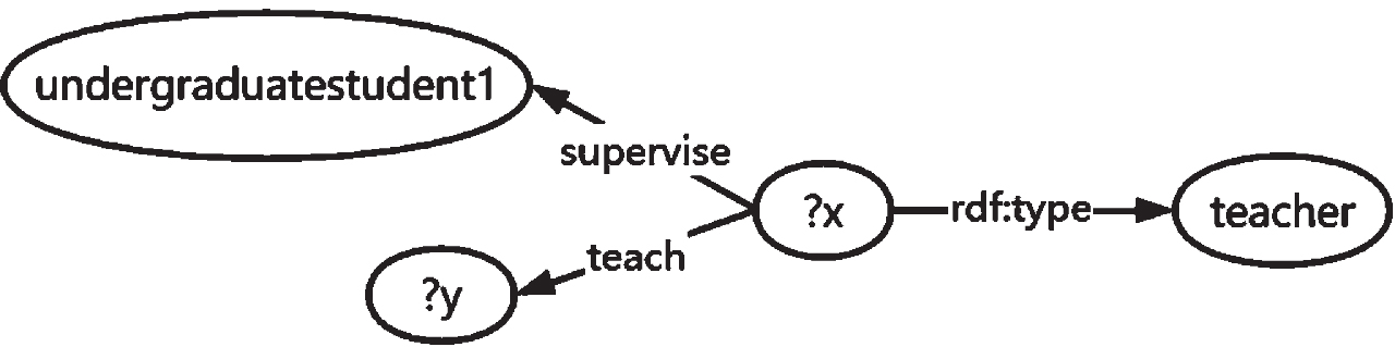
SPARQL query graph.

select ? x, ? y

where{ ? x supervise undergraduatestudent1

? x rdf:type teacher

? x teach ? y}

With the continuous expansion of application fields, people pay attention to the query efficiency of RDF data. The query methods of RDF data are divided into two types: triple-pattern query and keyword query. Triple-pattern query is one of the main RDF query methods [9], but because of not understanding the query language and underlying data structure, this query is not suitable for ordinary users, so the easy-to-operate keyword query is increasingly popular. However, in the face of the explosive growth of data scale, using keyword query technology directly on RDF data will cause problems like result redundancy and deviation. For example, keyword query in RDF graphs often results in a large number of information graphs containing keywords. At this time, if the structure and content of the RDF graph data are not considered, the precision rate will be reduced [13]. Therefore, how to perform accurate keyword search on large-scale RDF knowledge graphs has become a hot topic of research.

In [15], Peng et al. proposed that frequent query patterns are defined according to the frequency of subgraph query, and vertical fragments, horizontal fragments and mixed fragments are constructed to store the matching these frequent access patterns. Although refining the storage pattern is beneficial to store different frequent access patterns more finely, it will also prolong the search time and reduce the query efficiency in the process of constructing access patterns with different structures.

Facing the explosive growth of data scale, how to perform accurate search keywords on large-scale RDF graph has become a problem to be solved. It can be observed from Fig. 1 that there is an edge with a property of rdf:type pointing to a common node course for course1, course2, course3 and they have the same predicate edges takecourse and teach which frequently appear. So the course can be taken as the type of course1, course2, course3 and these instances can be stored in the patterns. We conclude that there are a large number of nodes of the same type in RDF data graph, and these nodes of the same type are often connected by the same predicate and we call these as pattern search triples or PST for short.

Based on this discovery, we extracted two actual RDF knowledge graphs data from DBpedia and LinkedGeoData, in which 25% of the PST accounted for 85% of the total number of PST, as shown in Fig. 3. This means that more than 85% of the PST in RDF graph only contain the most common 25% PST, so we define frequent search patterns to store the most common PST.

Fig. 3

Search data set.

The main contributions of this paper are as follows:

Based on the edge labels in RDF data graph, we obtain the types of subjects and objects, and construct RDF type graph.

The frequent search pattern is defined, and the lists from frequent search patterns to type instances are established to speed up the query.

Bloom coding is used to search whether the query information our need is in the frequent search pattern in a short time.

The effectiveness and efficiency of our method are evaluated on large RDF graphs. The experiments show that our method is much better than the existing methods in terms of precision and query response time.

The rest of this paper is organized as follows: Section 2 introduces related definitions and related work. Section 3 summarizes our approach. In Section 4, we introduced the type graph and the construction method of it. Frequent search pattern and Bloom coding are introduced separately in Section 5 and Section 6. The experiments are given in section 7. Section 8 concludes this paper.

2 Background

2.1 Definitions

Problem definition: given keyword set Q = {q₁, q₂,... q_i,...,. q_m} and RDF data graph G, the keyword search of the RDF graph is to find the result with the highest degree of matching with keywords.

Definition 1. (RDF triple) Given a URI set U, an empty node set B, and a text description set L, an RDF triple T is a group with the form of (subject, predicate, object), where subject ∈ U ∪ B, predicate ∈ R, object ∈ U ∪ B ∪ L. In the following chapters, s, p and o are used to represent the subject, property and object of the triple.

Definition 2. (RDF knowledge graph) RDF knowledge graph G denoted as a triple (V, E, L), where V is a vertex set corresponded to subjects and objects, E is an edge set corresponded to properties and L is a label set and L = L_v ∪ L_p, in which L_v is a label set of vertex, L_p is a label set of edge. That is, RDF knowledge graph is a graph with subjects and objects as vertexes, properties as edges, and labels on both vertexes and edges.

Definition 3. (RDF type graph) RDF type graph T is a triple (V’, E’, L’), with the object corresponding to the edge label rdf:type as its node type. If there is no rdf:type label, the node type is represented by ANYLABEL. And the subjects and objects of the triples are represented by their types in RDF data graph.

Definition 4. (triple pattern) Triple pattern t_p = (s_p, p_p, o_p) is a triple where s_p and o_p are represented by subject and object types.

Definition 5. (RDF keyword search) Given keyword sets k = k₁, k₂,..., k_n, the query result is a rootless graph G, where (1) for the keyword w_i ∈ k, G has nodes related to it; (2) the leaf node of G must be a keyword node.

2.2 Related work

Due to the complexity of Semantic Web query language, users prefer simple query pattern, while keyword search method can match query to RDF data graph only by inputting keywords, and our query result is the smallest graph obtained by connecting these keyword nodes. Semantic SPARQL similarity search over RDF knowledge graphs is proposed in [23]. Also, semantic SPARQL search considers the complex semantically equivalent graph structures, and does not support simple keyword search.

According to query processing methods, RDF keyword queries can be divided into three categories. The first category is to construct query results directly from query keywords [10, 12], and the second is to obtain query results after constructing structured query statements [7, 8]. The third category is document-centric keyword search [26, 28].

2.2.1 Query results obtained directly from keyword

In this method, the query result is obtained by defining the query result model and establishing related indexes. Since the data model of RDF is a graph, there are two methods to model the results. One is to model the query results as a tree, and the leaf nodes are used as keyword nodes, which are connected by other nodes in the tree. The results are to find the minimum query result trees, that is, Steiner trees, including [3, 4]. The other model the query results as graphs to find all the keyword nodes and the shortest paths between them, including [5, 6].

As the increasing number of Semantic Web data and user query, searching directly on the RDF data graph is inefficient, so this method needs to construct indexes to reduce the scale of RDF data graph. The index can be divided into keyword inverted index and structure index. By sorting the edge labels of nodes to form a sequence and designing a sequential pattern mining algorithm, a structural index based on frequent star patterns is established, and an inverted table is established for these sequential patterns to store the vertexes appearing in the sequential patterns [1]. In [2], Wu et al. proposed to partition the large RDF graph and summarize it. Three inverted indexes are established to record the entry node, root node and summary node of partition respectively.

The method of directly constructing query results only needs to match the results directly in the graph, which has the advantage of fine query granularity and does not need the support of RDF schema information [24, 27]. However, when RDF data is huge, it takes a lot of time and space to build indexes, which affects the query efficiency.

2.2.2 Query results obtained from query statements

By matching keywords to the nodes or edges of the data graph, with the help of pattern information, the relationship between user’s query objects and keywords is found, and structured query statements are constructed to retrieve the results [7, 8]. After the structural information extracted from RDF data graph and the query graph constructed, the sub-graph is converted into a structured query. And then the query result is generated by combining the index. Although this method is efficient, the data formed after abstraction is coarse in granularity and the query result may be inaccurate [11, 25].

2.2.3 Document-centric keyword search

The third method is document-centric keyword search, which concatenates the text contained in the nodes and edges of the RDF graph to the text document, and uses IR technology to ranking. In [26], a document-centric IR system is proposed for supporting keyword search over RDF datasets. In [28], Dosso et al. proposed the document-based keyword search system over large RDF datasets. This approach seems promising from a scalability point of view to avoid online graph traversal, which requires a lot of time and memory.

3 Overview

3.1 Storage structure

In this paper, RDF graph information is stored in the form of adjacency list, that is, a single linked list is created for the subject nodes in the graph to store the subject and its type information. Here, we call it the head node (such as teacher1), and each head node connects the predicate edges and the object nodes connected with the subject node (such as teacher1 and undergradedstudent2 connected through teach. Therefore, the head node teacher1 points to teach and undergraduatestudent2), in which we call them tail nodes (such as teacher). The data structure of Fig. 1 is shown in Fig. 4 and Fig. 5.

Fig. 4

Adjacent table data structure.

Fig. 5

Adjacent table data structure.

We use AdjList[i] to represent the head node array, the “subject” and “type” in the head node respectively represent the IDs corresponding to the subject and subject type, the linked list “next” is connected to the tail node ArcNode corresponding to the head node, and the “property” and “object” in the tail node are respectively represents the IDs of the predicate and object in the data graph and “next” connects to the next predicate and object connected to the subject.

In order to save space, we can also assign the entities (for example, graduate1), predicates (for example, takecourse) and types (for example, teacher) in the graph to IDs. The specific information is shown in Table 1. In the data structure of Fig. 4, we use the IDs value of Table 1 to indicate the corresponding subject predicates and type values.

Table 1

IDs of entities, predicates and types

(a) Entity table
Entity Name	id
undergradutatestudent1	1
undergradutatestudent2	2
undergraduatestudent3	3
teacher1	4
teacher2	5
course1	6
course2	7
course3	8
graduatestudent1	9
graduatestudent2	10
(b) Edge label table
Edge label	id
rdf:type	0
takecourse	11
supervise	12
teach	13
(c) Type table
Type	id
undergraduatestudent	14
teacher	15
course	16
graduatestudent	17
ANYLABEL	18

In order to facilitate the calculation of frequent search patterns, we define an inverted list to store frequent search patterns and their corresponding instances.

3.2 Overview of the methods

The framework diagram and the flow diagram of our solution are shown in the Fig. 6 and Fig. 7, which mainly includes the following steps:

Fig. 6

Framework diagram of our solution.

Fig. 7

Flow diagram of our algorithm.

Step 1. According to the edge label rdf:type, retrieve the types of each node in RDF data graph, and edges with rdf:type attributes and type nodes are deleted.

Step 2. For each query pattern triple p, find the number of occurrence times in RDF data graph, and filter out the average frequency pattern whose occurrence times exceed PST as frequent patterned search triple FPST, and combine FPSTs with the same subject type to form frequent search pattern FSP.

Step 3. Define an inverted list and add instances for each frequent search pattern.

Step 4. Select several Hash functions and build a Bloom coding. Then encode the subjects, predicates and objects in each frequent search pattern and carry out OR operation on the obtained codes to acquire Bloom coding of each frequent search pattern.

Step 5. For a given keyword search, judge the types of keyword and decompose them into several query patterns.

Step 6. Encode the query modes in the same way as step 4, and perform an AND operation with the Bloom coding of the corresponding frequent search patterns to determine whether each query pattern belongs to the frequent search patterns.

Step 7. If it is a frequent search pattern, search the inverted list to return the query results.

4 Type graph

In this section, we discuss how to transform RDF knowledge graph into type graphs, which is also the key step to simplify the algorithm in this paper.

4.1 Node type

We have observed that rdf:type is often used in RDF graphs to illustrate that an entity is an instance of a certain class, and nodes of the same type are often connected by the same predicate, so we can find many patterns with the same structure. We take all the objects with rdf:type as the subject types in RDF graph, so that we can reduce the scale of RDF graph by merging the subject and object with the predicate as rdf:type and deleting the rdf:type edges and the type nodes connected to it.

Taking Fig. 1 as an example, undergraduatestudent1, teacher1, graduatestudent1 and course1 take the objects connected by rdf:type as their node types, that is, their types are undergraduatestudent, teacher, graduatestudent and course respectively. However, in practice, not all nodes have rdf:type edges, so we define this node type as ANYLABEL, which means that this type can match any node. The simplified RDF graph of Fig. 1 is shown in Fig. 8.

Fig. 8

RDF type graph.

4.2 The construction of type graph

The construction of the RDF type graph is shown in Algorithm 1.

Algorithm 1
Input: Graph G
Output: Type Graph T
1. for(v = 0; v <G.vexnum; v++)
2. p = AdjList[v];
3. while(p->next)
4. if(p->next.property = =0)
5. AdjList[v].type = p.property;
6. p->next = p->next->next;
7. p = p->next;
8. if(!AdjList[v].type)
9. AdjList[v].type = 17;

Firstly, we traverse the adjacency table of the RDF graph in a breadth-first form. When the attribute value is rdf:type, we store its corresponding object in the type of the head node, and delete this node and attribute edge (lines 4–6). If the rdf:type attribute does not exist in the head node, ANYLABEL is stored in the type of the head node (line 8-9). The time complexity of the algorithm is O(n), where n is the number of nodes in RDF graph.

5 Frequent search pattern

5.1 Definition

Given the frequent search pattern FSP, if FSP can match part of the subgraphs of the RDF graph, the FSP can be used to search queries containing this pattern, which can greatly speed up the query. And the more queries FSP hits, the faster the query speed. At the same time, if too many frequent search patterns are established, the space cost will be too high. Therefore, we give the following definition.

Definition 6. (pattern search triple) Let U be an infinite set containing all URIs and V be an infinite set containing all types, then t = (S, P, O) = V × U × V is called a pattern search triple (PST for short).

Definition 7. (frequent pattern search triple) Given the PST set P = p₁, p₂,..., p_n contained in the data set. For p_i ∈ P, the number of times it appears in W is n. Then When the frequency of p_i is $f i = \frac{ni}{\sum_{j = 1}^{n} nj} \frac{k}{| P |}, 0 < k 1$ (1)

P_i is a frequent pattern search triple (i.e. FPST).

The value of k in definition 7 determines the lowest frequency meeting the condition of “frequent”, when k = 1, it means that a PST is frequent when its frequency is not lower than the average frequency of all PSTs. The smaller the value of k is, the more frequent PSTs are. Until k = 0, all PSTs are frequent. Decreasing the value of k is beneficial to more PSTs becoming FPST, but since many PSTs appear less frequently, incorporating them into frequent PSTs requires larger storage space and higher maintenance costs. In this paper, we take k = 1, that is, a PST is a frequent PST when its frequency is not lower than the average frequency of all PSTs.

Definition 8. (frequent pattern search) For frequent pattern search triples (S, P, O), if S (i.e. subject) is the same subject type, they can merge, and the merged graph is called frequent search pattern, namely FSP.

Taking Fig. 1 as an example, where ∑n = 10, for PST(teacher, teach, course) and PST(teacher, supervisor, undergraduatestudent), whose occurrence number are all n = 3 and frequency are all f = 3/10 >1/4. Therefore, there are two FPSTs of the type teacher, and they are merged as shown in Fig. 9. Here, in order to intuitively represent the search model, the node information is not represented by the IDs, and the IDs are used to store the node information in the actual storage.

Fig. 9

Frequent search pattern.

5.2 Construction of frequent search pattern

This section introduces the algorithm for calculating frequent search patterns. The algorithm extracts the pattern search triple (PST) from the type graph obtained in Section 4 and calculates the frequent pattern search triple (FPST) according to formula 1. Finally, we combine the frequent pattern search triples (FPSTs) with the same subject type to get the frequent search pattern (FSP). In order to facilitate search space, we establish an inverted list from frequent search patterns to their subject instances. Since the data graph is stored by adjacency table, it can be directly located in RDF graph according to subjects.

The specific steps are as follows: first, we traverse the type graph T, extract the subject type stype, the predicate p.property and the object type otype of the search pattern (lines 2–9). And then the search patterns are stored in array pattern[i] (lines 11 and 14) while the corresponding instances of their subject are stored in pattern[i][j] (lines 12 and 15); Calculate the average frequency of PST, filter out the frequent pattern search triple (FPST) and store it in P (lines 18-19). Then frequent search patterns with the same subject type are combined and stored in FSP and an inverted list is built to store the subject instances of frequent search patterns (line 20 and 21).

Algorithm 2
Input: Type Graph T
Output: the frequent search pattern FSP
1. i = 0;
2. for(v = 0; v <T.vexnum; v++)
3. p = AdjList[v]->next;
4. stype = AdjList[v].type;
5. sentity = AdjList[v].subject;
6. while(p)
7. if(p.property ! = 0)
8. oentity = p.object;
9. otype = AdjList[oentity].type;
10. if (stype, p.property, otype) not in pattern[i]
11. pattern[i++] = (stype, p.property, otype);
12. add sentity in pattern[i][j];
13. else
14. i = arg(pattern[i] = (stype, p.property, otype));
15. add sentity in pattern[i][j];
16. p = p->next;
17. for(i; i> = 0; i–)
18. if ( $\frac{pattern[i].length}{T.arc}$ > = $\frac{1}{\| P \|}$ )
19. P = pattern[i];
20. FSP is connect the same stype in p[i]
21. FSP->next = sentity in pattern[i][j]

6 Keyword search based on type graph

6.1 Bloom Filter

If we want to judge whether an element is in a set, the traditional method is to traverse each element in the set in turn, and then determine it by comparison. However, with the increase of elements in the collection, we need more and more storage space, and the retrieval speed will be slower and slower. At this time, we use the data structure of Hash table. It can map an element to a point in a bit array through a Hash function. In this way, we only need to see if this position is 1 to know if this element is in the collection and that is the basic idea of Bloom Filter. Below we give the definition of Bloom Filter.

Bloom Filter is composed of a binary vector and a series of random mapping functions, which can be used to retrieve whether an element is in a set. Its advantage lies in higher space utilization and faster query efficiency, while the disadvantage is that it has a certain misjudgment rate, that is, elements that are not in the set may be misjudge as elements of the set, but there will be no false negative.

Establishment of Bloom Filter: firstly, a bitmap with m bits is established, and each bit is set to 0. For each added element, k hash functions are used to map k hash values to k positions of the bitmap. And then all bits of these k positions are set to 1. When searching, we only need to search whether these k bits are all 1s: if any of these bits is 0, the checked element must not be there; If they are all 1, the checked element is likely to exist.

The false positive rate of the Bloom Filter: Assume that the Bloom Filter has m bit, n elements to be detected by k Hash functions, then the probability when a certain bit position is 1 is $\frac{1}{m}$ , and the probability that it is still 0 is $1 - \frac{1}{m}$ .

For a certain position of the filter, the probability that the bit is not set to 1 after all k Hash operations is $(1 - {\frac{1}{m})}^{k}$ . When we insert n elements, the probability that a certain bit is still 0 is $(1 - {\frac{1}{m})}^{kn}$ . So, the probability that this bit is 1 is $1 - (1 - {\frac{1}{m})}^{kn}$ .

Now suppose that these n elements are all placed in the Bloom Filter. For an element that is not in the set, the probability that its first hash function just hits 1 is the above probability, and the probability that all k Hash functions hit 1 is the misjudgment rate, and its probability is: $[1 - (1 - \frac{1}{m})^{kn}]^{k} \approx (1 - e^{- kn / m})^{k}$ .

In fact, the above results assume that the positions of the bits that need to be set calculated by each hash function are independent of each other. It is not difficult to see that as m (bit array size) increases, the misjudgment rate will decrease. And at the same time, as the number of inserted elements n increases, the misjudgment rate will rise again. For a given m, n, when $k = \frac{m}{n} ln 2 \approx 0.7 \frac{m}{n}$ , the misjudgment rate p is the smallest, that is p = 2^-k ≈ 0 .6185^m/n.

And when the false positive rate is not greater than

e, we can get $m ⩾ - \frac{n ln p}{{(ln 2)}^{2}}$ . In other words, in order to guarantee the false positive rate, m must be at least equal to $- \frac{n ln p}{{(ln 2)}^{2}}$ .

6.2 Bloom coding

Definition 8. (Bloom coding) Each frequent pattern search triple in the frequent search pattern in RDF graph is coded according to Bloom filter, and the coding obtained by bitwise-or operation is called Bloom coding.

As shown in Fig. 10, for the convenience of presentation, here we choose 8-bit bitmap and two Hash functions APHash and JSHash as demonstration. The dashed line in Fig. 10 represents the coding and the solid line represents the calculation. Taking the frequent search pattern in Fig. 9 as an example. Firstly, we obtain the hash values of the first pair of patterns, APHash(teacher) (2147383290) and JSHash(teacher) (2762490817), APHash(teach) (2147383292) and JSHash(teach) (2762490823), APHash(course) (2147383289) and JSHash(course) (2762490816). And get the remainders 3, 6 and 5, 5 and 2, 1 obtained for these six Hash values mod 8. Then, the 3rd and 6th positions of array1 from right to left are 1, the rest positions are 0, the 5th position of array2 from right to left is 1, the rest positions are 0, and the 2nd and 1st positions of array3 from right to left are 1 (starting from the 0th bit). Similarly, the vertex teacher and undergraduatestudent are mapped to a bit array with a length of 8, and the values of APHash and JSHash functions are taken to mod 8 to get the remainder for coding; Finally, the codes of different outgoing edges are bitwise-or operated to obtain the Bloom coding of frequent search pattern.

Fig. 10

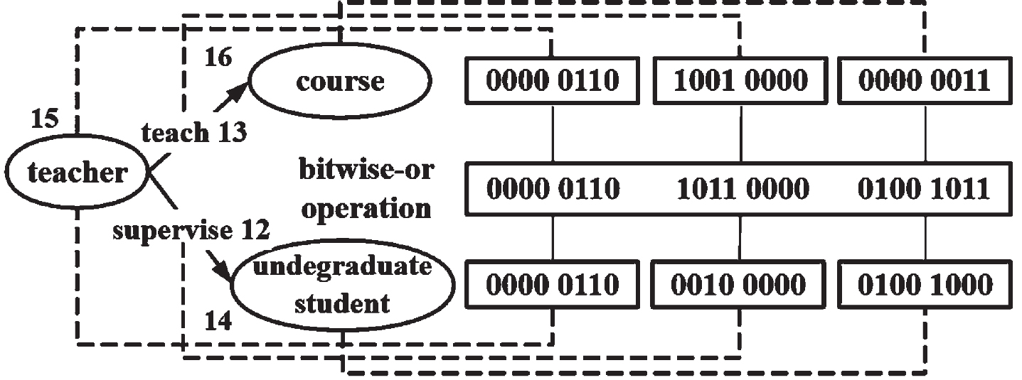
Bloom coding of frequent search pattern.

Looking back at the query put forward in the first section, “Search the course taught by the teacher of undergraduatestudent1”, the keywords in this query are undergraduatestudent1, supervise, teacher, teach. Find the corresponding types of the keywords, and its search pattern is shown in Fig. 11. Among them, we know two subject types (undergraduatestudent and teacher) and two predicates (supervise and teach), and the course is a variable, so its 8-bit Bloom coding is set to 1. According to the above method, the hash code of the query pattern is obtained and converted into Bloom coding. The result of AND operation between the query code and the Bloom coding is equal to the frequent pattern code, indicating that the query is in the frequent pattern.

Fig. 11

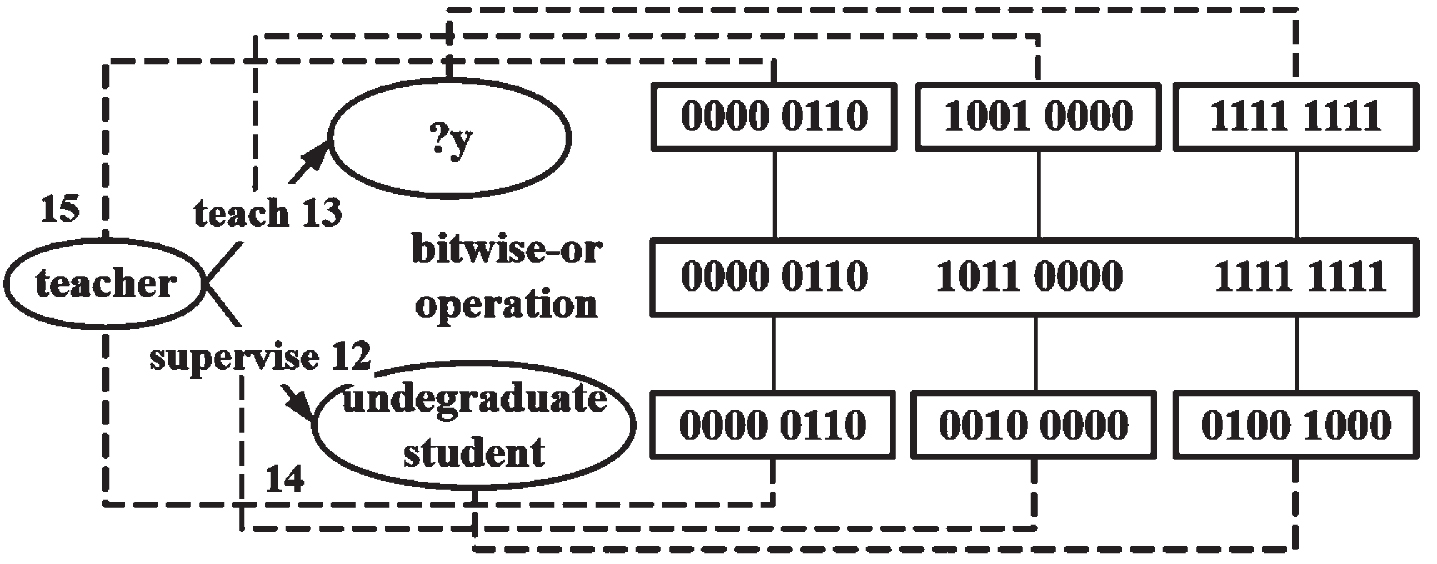
Bloom coding of the keywords and search pattern.

6.3 Query algorithm

The query algorithm is shown in Algorithm 3. Assuming that the query graph stored in an adjacency table, the subjects in the query graph are stored in the head nodes of the adjacency table. First, for the pattern in the query graph, we calculate its Bloom coding and combines it with the code of frequent search patterns in AND operation. If the result is equal to the code of frequent pattern, the query is in frequent pattern (lines 1–4). Next, we judge whether the subject is a variable. If it is a variable, we need to find the corresponding subject instances in the inverted list of frequent search patterns (lines 5–8). For the searched subject instances, we find the corresponding predicate and object instances from the adjacency list of RDF graph, and make them into sequences (subject and object) (lines 9-10), and connect the results of all sequences to get the query answers (line 11).

Algorithm 3
Input: Query Q, FSP
Output: Answer
1. for v in QList
2. bcv = Bloom coding of v;
3. bcFSP = Bloom coding of FSP;
4. if bcv &bcFSP = =bcFSP
5. if v is variable
6. while(FSP->next)
7. if(v = =FSP->next)
8. subject = =v;
9. search object in AdjList[subject];
10. add (subject, object) in candicate;
11. Answer = connect candicate;

7 Experiment

7.1 Experiment environment and date sets

The workstation hardware environment used in this experiment is Intel(R) Core(TM) i7-7700 quad-core processor, its memory size is 16GB, the hard disk size is 500GB, and the communication between nodes uses 1000Mbps Ethernet. The experimental platform uses Linux 64-bit CentOS operating system. We use two real data set DBpedia and IMDB and a synthetic data set LUBM(Lehigh University Benchmark) for experiments. The basic parameters of the data set are described in Table 2.

Table 2
Dataset parameters

Number of triples/ten thousand Number of types Files size/GB

LUBM50 691 32 0.51

LUBM200 3235 32 2.39

LUBM500 6917 32 5.36

DBpedia 607 134 0.91

IMDB 316 98 2.1

	Number of triples/ten thousand	Number of types	Files size/GB
LUBM50	691	32	0.51
LUBM200	3235	32	2.39
LUBM500	6917	32	5.36
DBpedia	607	134	0.91
IMDB	316	98	2.1

The data sets are introduced as follows:

DBpedia: DBpedia [21] is an RDF data set extracted from Wikipedia. We use DBpedia SPARQL query log [14] as the workload, in which there are 8,151,238 queries.

IMDB: IMDB [30] is an international movie dataset of 2.1 GB and we converted it into an RDF dataset of about 3164 thousand triples.

LUBM: LUBM [29] is a database of universities, professors and students developed by Lehigh university. This paper uses LUMB data generator to generate data of 50, 200 and 500 universities as test data sets respectively.

The search examples used in this experiment are shown in Table 3. There are 15 keyword sets Q₁-Q₁₅ in total, and each keyword set contains 2-5 keywords, including instance, attribute and type keywords. In the query keywords Q₁-Q₁₀, except for the keywords “ Graduatestudent0” and “ Teacher4”, the other keywords are all selected from several universities from the LUBM dataset. And in the query keywords Q₁₁-Q₁₅, all keywords are selected from the IMDB dataset. In order to simulate the situations in the real datasets, all the keywords in the query are not close to each other. The algorithm in this paper is compared with the existing keyword search algorithms SUMM [12] and SCHEMA [14].

Table 3

Search example

Queries	Short description
Q ₁	Department3, University1, Professor5
Q ₂	Graduatestudent0, Research8, Teacher1
Q ₃	teach, Undergraduatestudent0, Graduatestudent1, Teacher
Q ₄	China, birthpalce, professor, Harvard University
Q ₅	Mark, Graduatestudent, Teacher8, Math
Q ₆	C, Takecourse, Graduatestudent, Undergraduatestudent
Q ₇	C++, Mark, teach, Teacher4
Q ₈	College, Computer Science, Course
Q ₉	Professor7, Lecture3, Publish
Q ₁₀	Lecture3, Publication10
Q ₁₁	Thriller movie, Act, Actor
Q ₁₂	Philadelphia, wonPrize, ActressAcademyAward
Q ₁₃	Will Ferrell, Rating
Q ₁₄	Superman movie, Company, Actress
Q ₁₅	MelanieGriffith, Birthplace

7.2 Selection of hash function

In order to select the appropriate Hash function in Bloom Filter, we compared the performance of several commonly used hash functions. As shown in Table 4, we selected four types of data for experiments, namely 100,000 random strings composed of letters and numbers, 100,000 meaningful English sentences, taking 100,000 random strings composed of letters and numbers modulo 1000,003 (large prime number) modulo and taking the random strings consisting of 100,000 letters and numbers modulo 10,000,019 (larger prime number). The number of hash conflicts obtained are stored in data 1 to 4 respectively, and the scores of data 1-4 are calculated by the following formula: $\begin{matrix} score i = \\ \frac{100}{max (data) - min (data)} * (max (data) - datai) \end{matrix}$ (2) where, max(data) and min(data) represent the maximum and minimum values of the number of conflicts in the current experiment respectively, and (max(data) - data_i) represents the difference between the number of conflicts in this function and the maximum number of conflicts in the current experiment.

Table 4

Hash function comparsion

	Data1	Data2	Data3	Data4	Data score1	Data score3	Data score4	Average score
BKDRHash	2	0	4771	482	96.55	93.09	100.00	97.45
APHash	2	3	4756	493	96.55	100.00	66.67	88.87
DJBHash	2	2	4973	507	96.55	0.00	24.24	67.88
JSHash	1	4	4756	504	100.00	100.00	33.33	84.07
RSHash	1	0	4867	506	100.00	48.85	27.27	76.04
SDBMHash	3	2	4923	501	93.10	23.04	42.42	69.86
PJWHash	29	25	4874	515	3.45	45.62	0.00	22.96
ELFHash	30	26	4876	513	0.00	44.70	6.06	22.55

We calculate the square average based on the scores of the four data, and the formula is as follows: $\begin{matrix} average_score = \\ \frac{\sqrt{score 1^{2} + score 2^{2} + score 3^{2} + score 4^{2}}}{2} \end{matrix}$ (3)

We can find that BKDRHash has the most outstanding effect both in actual effect and coding implementation. APHash is also an excellent algorithm, while DJBHash, JSHash, RSHash and SDBMHash also have their own advantages. PJWHash and ELFHash have the worst effect, but their scores are similar, and essential of their algorithms are similar.

7.3 Choice of number of array bits and hash functions

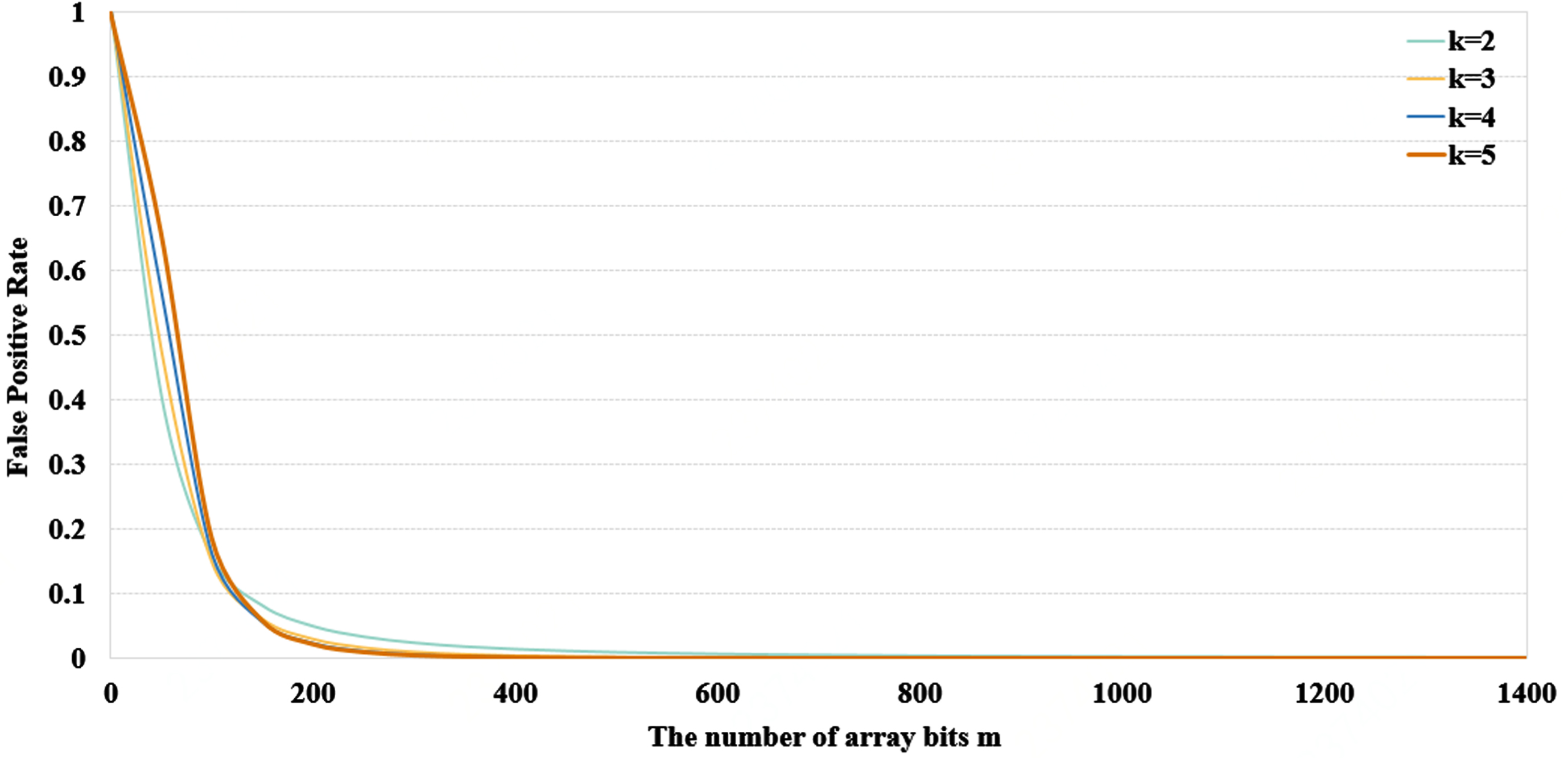
This group of experiments assumes that each frequent search pattern has 25 branches respectively, and the number of Hash function is set k = 2, 3, 4, 5. According to the error rate formula $P = [1 - (1 - {\frac{1}{m})}^{kn}]^{k}$ (refer to Section 6.1), the image is shown in Fig. 12 which compares the influence of the number Hash function and the number of array bits on the misjudgment rate. To ensure the misjudgment rate is below 0.1%, we need to set k = 2, m = 13000 or k = 3, m = 650 or k = 4, m = 500 or k = 5, m = 400. When the number of array bits exceeds 200, the increase in the number of Hash functions or the increase in the number of array bits in the array will reduce the misjudgment rate. Although the increase of Hash functions is conductive to reducing the memory space occupied by the array, it will also increase the cost of computing and searching data and then affect the search efficiency.

Fig. 12

The change of misjudgment rate when changing the number of hash functions k and the number of array bits m.

To compare the search efficiency when k = 2, m = 1300 or k = 3, m = 650 or k = 4, m = 500 or k = 5, m = 400, we conducted 10 sets of queries on the data set LUBM500. As shown in Fig. 13, we found that when the misjudgment rate is 0.1%, no matter what kind of queries, the query efficiency is always highest.

Fig. 13

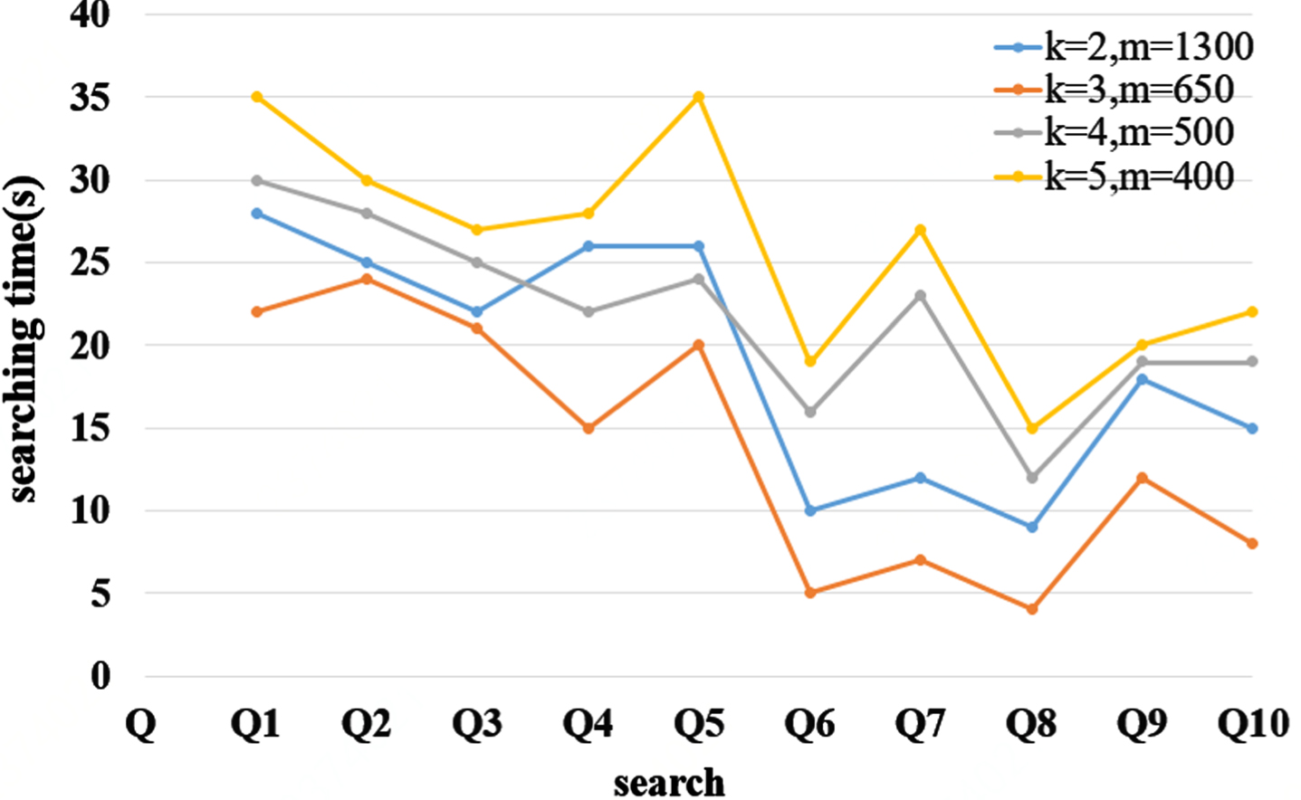
The number of Hash functions and the choice of array bits.

7.4 Experiment result

This section introduces the experiment in detail from three aspects, including precision, recall and search efficiency test. In the experiment, the number of Hash functions is set to 3, and the number of array bits is set to 650. In order to ensure the accuracy of the experimental results, the average value of each query test is taken three times to avoid random errors.

7.4.1 Precision and recall

Precision is used to measure the accuracy of Top-k search results, which is the ratio of the number of correct instance triples in search results to the total number of instance triples in search results. The Recall is the ratio of the number of correct case triples in the search results to the total number of related case triples in the data set. For the queries Q₁-Q₁₅, we know the number and range of answers, so we can calculate the number of the following three parameters. And for different data sets, create a set for each search example, which is used to store all the search results related to the search example. The definition of precision and recall are as follows: $\begin{matrix} Precision = \\ \frac{Number of correct instance triples in search results}{Total number of instance triples in search results} \end{matrix}$ (4) $\begin{matrix} Recall = \\ \frac{Number of correct instance triples in search results}{Number of related instance triples in set} \end{matrix}$ (5)

Figures 14 and 15 show the comparison of the precision and recall of the three algorithms under the LUBM500, DBpedia and IMDB data sets. As shown in Fig. 14, for queries Q₁-Q₁₅, the average precision rates of OURS, SUMM and SCHEMA in three datasets are 0.913, 0.7863 and 0.7227, respectively. Compared with SUMM [12] and SCHEMA [14], the average accuracy of our algorithm is improved by 16.10% and 26.34%. In this paper, Bloom coding is used to judge whether the query matches the existing frequent search patterns. If matches, the search results can be obtained by querying the inverted list of examples, so regardless the possible misjudgment of Bloom coding, we can get accurate results regardless the possible misjudgment of Bloom coding. Through the experiment in Section 7.3, we can set the number of hash functions k = 3 and the number of array bits m = 650 to ensure that the misjudgment rate is below 0.1%. Fig. 15 shows that the search precision of the third, fifth, sixth and fifteenth groups of the algorithm in this paper is higher than that of other groups. The reason is that these three groups of searches contain more types of keywords and more comprehensive information, so less search results is returned, besides returning correct search results, other results indirectly related to keywords will be returned during approximate search. It can be seen from Figs. 14 and 15, for queries Q₁-Q₁₅, the average precision rates of OURS, SUMM [12] and SCHEMA [14] in three datasets are 0.909, 0.78 and 0.7237, respectively. Compared with SUMM and SCHEMA, the average accuracy of our algorithm is improved by 16.54% and 25.61%. And the recall ratio of queries Q₁ to Q₃ and Q₁₃ to Q₁₄ of searches in this algorithm is low, while the recall ratio of the other queries is high, which is because the Top-k result has already been satisfied without returning all the correct case triples in the first three groups of searches, and some correct case triples are omitted, resulting in low recall ratio.

Fig. 14

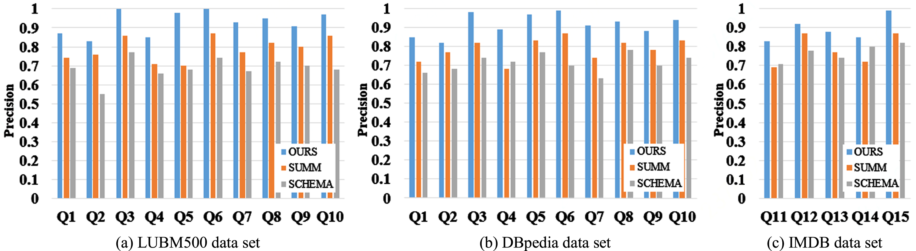
Comparison of precision rate of each algorithm under LUBM500 data sets.

Fig. 15

Comparison of recall rate of each algorithm under LUBM500 data sets.

7.4.2 Query efficiency test

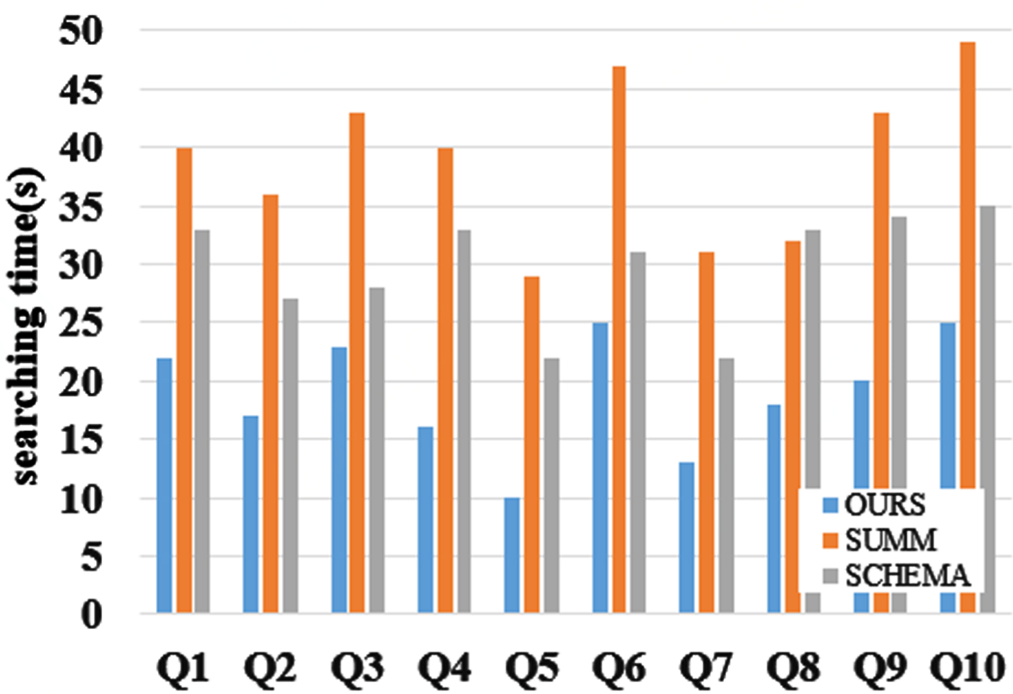
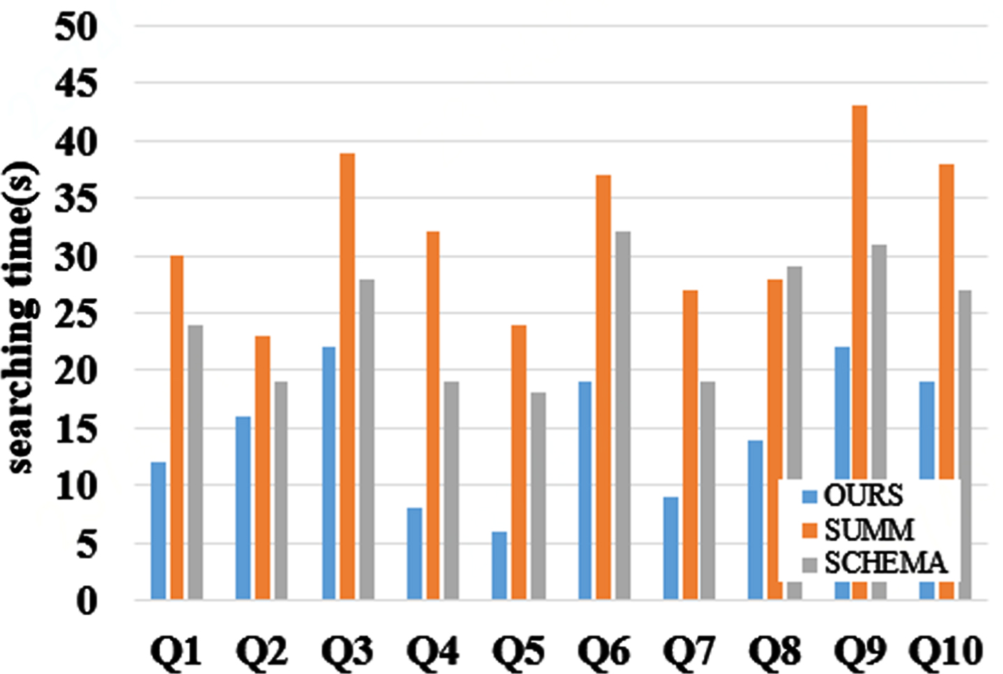
This group of experiments test the corresponding time of Q₁-Q₁₅ of our algorithm, SUMM [12] and SCHEMA [14] algorithms under LUBM500 data set and DBpedia data set. As shown in Fig. 16 and Fig. 17, for queries Q₁-Q₁₅, the average precision rates of OURS, SUMM and SCHEMA in three datasets are 16.8, 35.55 and 27.2 respectively and our algorithm can achieve the highest query efficiency in 10 keyword queries. Compared with SUMM [12] and SCHEMA [14], the average accuracy of our algorithm is improved by 16.54% and 25.61%. The reason is that SUMM method needs to partition millions of subgraphs and then divide them. However, our algorithm only builds a frequent search pattern based on types, and the frequent search pattern we built can cover most of searches, thus improving the query efficiency. For the third, the ninth and the tenth group, the query time is slightly higher than other queries, because these three groups have more query variables and fewer examples, and they will produce more query results and spend more time. Comparing the data sets LUBM500 and DBpedia, we can see that although the number of LUBM500 triples is nearly 11 times that of DBpedia, the search time difference between the two data sets is not so big, because the data set generated by LUBM500 is only related to schools, and its node types are much fewer than those of DBpedia. Even though the number of LUBM500 triples is larger, the query efficiency will not be greatly affected.

Fig. 16

Comparison of search response time of each algorithm under LUBM500 data sets.

Fig. 17

Comparison of search response time of each algorithm under DBpedia data set.

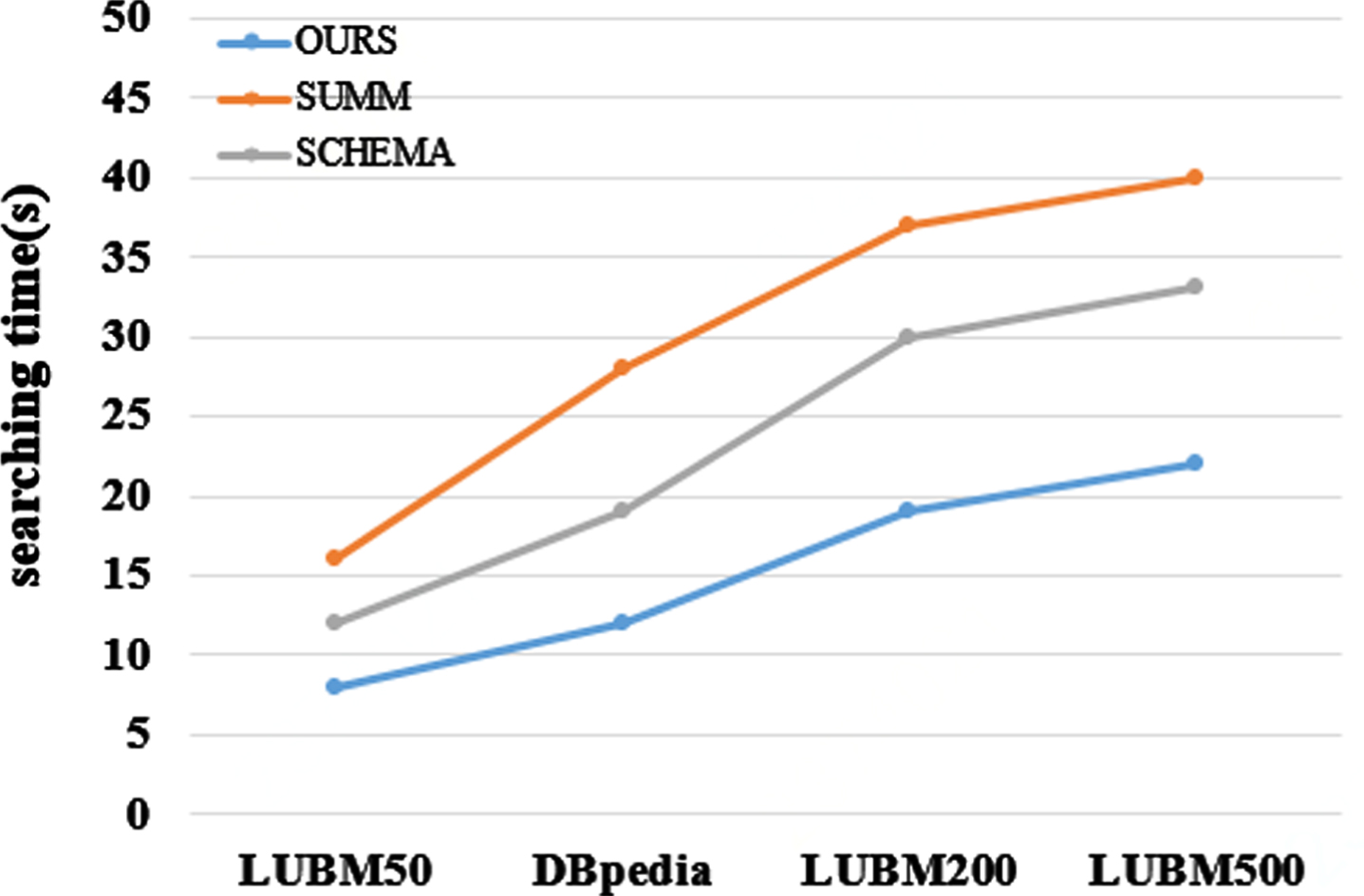
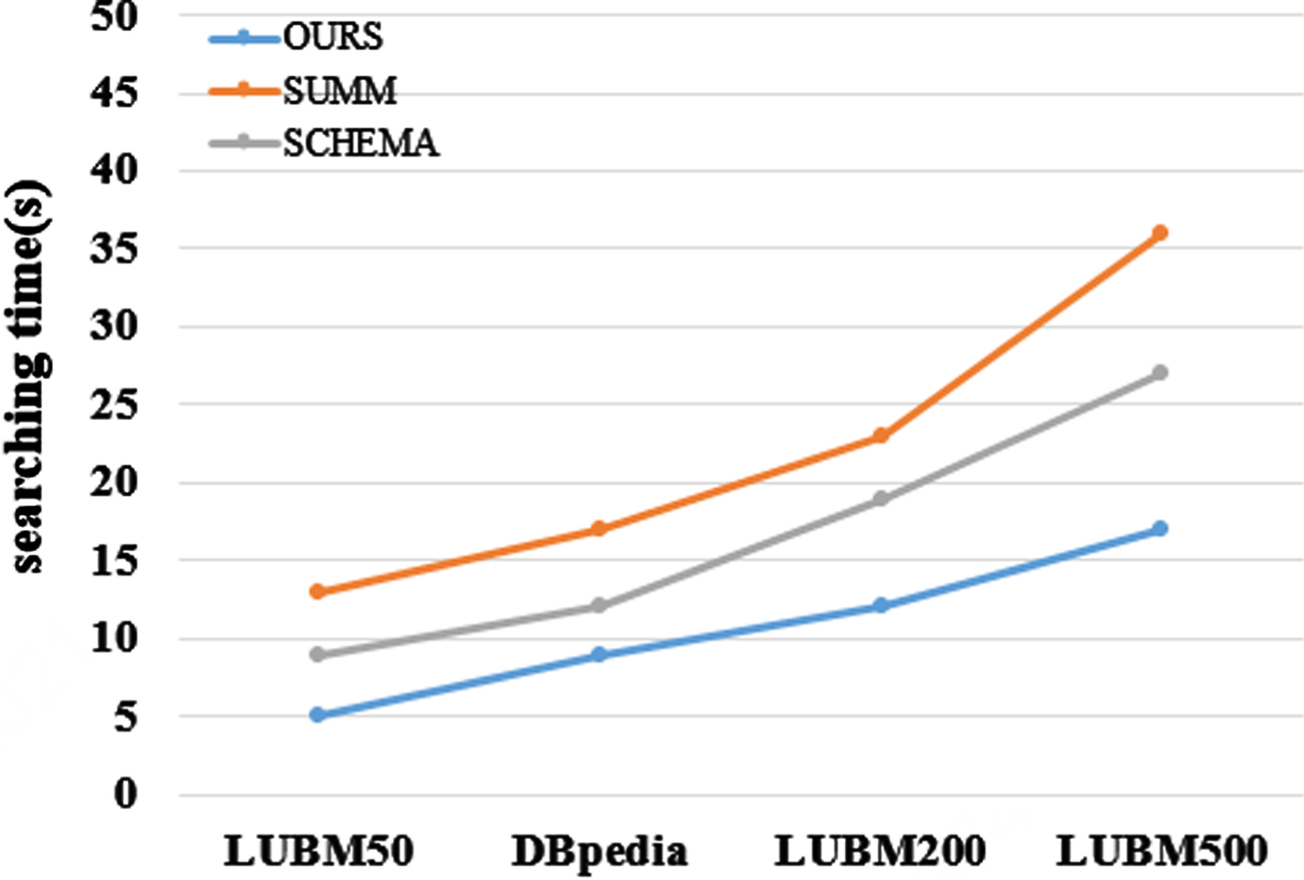
Figures 18 and 19 respectively show the query time of the three algorithms for Q₁ and Q₂ under the LUBM500 dataset. SCHEMA [14] method can only save one kind of relationship between different entities, which leads to a decrease of search efficiency in the summary graph. However, our method can save the relationship of all entities in frequent search pattern. It can be seen that with the increase of data amount, the query speed of this method increases linearly but the overall change is not significant. This is because as the number of RDF triples increases, RDF types and frequent patterns will not change significantly, while the query time of SUMM [12] and SCHEMA [14] increases greatly. Therefore, whether for different queries or for different data sets, the query efficiency of our algorithm is far superior to SUMM [12] and SCHEMA [14] algorithms.

Fig. 18

Comparison of average response time of two groups of queries under LUBM500 data set.

Fig. 19

Comparison of average response time of two groups of queries under DBpedia data set.

8 Conclusion

In this paper, a keyword search algorithm based on RDF type graph is proposed, which makes use of the repetitiveness of RDF node types to reduce the scale of RDF data graph. We also propose the pattern search triple (PST) and calculate the frequent pattern search triple (FPST). Then We merge these FPSTs with the same subject type and establish an inverted list from them to type instances, which is convenient for us to quickly find instances that meet the patterns. In order to speed up the query, this paper uses Bloom coding to judge whether the query information we need is in frequent search patterns.

In the future, we will investigate a more accurate keyword extraction algorithm, and combine this algorithm with distributed database to further improve the query efficiency of our algorithm.

Footnotes

Acknowledgments

The authors would like to express their gratitude to the anonymous reviewers for their valuable comments and suggestions.

References

Peng

, Zou

and Qin

, Answering top-K query combined keywords and structural queries on RDF graphs, Information Systems 67 (2017), 19–35.

, Zhou

, Yuan

, Liu

and Jin

, Scalable SPARQL querying using path partitioning, Proceedings of the 31st IEEE International Conference on Data Engineering, (2015), pp. 795–806.

Kasneci

, Ramanath

, Sozio

, Suchanek

F.M.

and Weikum

, STAR: steiner-tree approximation in relationship graphs, Proceedings of the 25th International Conference on Data Engineering, (2009), pp. 868–879.

Ding

, Yu

J.X.

, Wang

, Qin

, Zhang

and Lin

, Finding top-k min-cost connected trees in databases, Proceedings of the 23rd International Conference on Data Engineering, (2007), pp. 836–845.

, Wang

, Yang

and Yu

P.S.

, BLINKS: ranked keyword searches on graphs, Proceedings of the ACM SIGMOD International Conference on Management of Data, (2007), pp. 305–316.

Lian

, Hoyos

E.D.

, Chebotko

, Fu

and Reilly

, K-nearest keyword search in RDF graphs, Journal of Web Semantics 22 (2013), 40–56.

Gkirtzou

, Papastefanatos

and Dalamagas

, RDF keyword search based on keywords-to-SPARQL translation, Proceedings of the First International Workshop on Novel Web Search Interfaces and Systems, (2015), pp. 3–5.

Zenz

, Zhou

, Minack

, Siberski

and Nejdl

, From keywords to semantic queries-incremental query construction on the semantic Web, Journal of Web Semantics 7(3) (2009), 166–176.

RDF model and syntax specification, http://www.w3.org/TR/1999/REC-rdf-syntax-19990222/, 1999.

10.

Elbassuoni

, Effective searching ofRDFknowledge bases, Saarland University, 2012.

11.

Ladwig

and Tran

, Combining query translation with query answering for efficient keyword search, Proceedings of the Semantic Web: Research and Applications, 7th Extended Semantic Web Conference, 2010, pp. 288–303.

12.

, Li

, Kementsietsidis

and Duan

, Scalable keyword search on large RDF data, IEEE Transactions on Knowledge and Data Engineering 26(11) (2014), 2774–2788.

13.

Bhalotia

, Hulgeri

, Nakhe

, Chakrabarti

and Sudarshan

, Keyword searching and browsing in databases using BANKS, Proceedings of the 18th International Conference on Data Engineering, 2002, pp. 431–440.

14.

Tran

, Wang

, Rudolph

and Cimiano

, Top-k exploration of query candidates for efficient keyword search on graph-shaped (RDF) data, Proceedings of the 25th International Conference on Data Engineering, (2009), pp. 405–416.

15.

Peng

, Zou

, Chen

and Zhao

, Adaptive distributed RDF graph fragmentation and allocation based on query workload, IEEE Transactions on Knowledge and Data Engineering 31(4) (2019), 670–685.

16.

Mountantonakis

and Tzitzikas

, Content-based union and complement metrics for dataset search over RDF knowledge graphs, Journal of Data and Information Quality 12(2) (2020), 10:1–10:31.

17.

Shan

, Li

and Chen

, Constructing target-aware results for keyword search on knowledge graphs, Data and Knowledge Engineering 110 (2017), 1–23.

18.

Virgilio

R.D.

, Efficient and effective ranking in Top-k exploration for keyword search on RDF, Proceedings of the IEEE International Conference on Information Reuse and Integration, (2011), pp. 66–70.

19.

Lin

, Ma

Z.M.

and Yan

, RDF keyword search using a type-based summary, Journal of Information Science and Engineering 34(2) (2018), 489–504.

20.

Ladwig

and Tran

, Combining query translation with query answering for efficient keyword search, Proceedings of the Semantic Web: Research and Applications, (2010), pp. 288–303.

21.

Lehmann

, Isele

, Jakob

, Jentzsch

, Kontokostas

, Mendes

P.N.

, Hellmann

, Morsey

, Kleef

P.V.

, Auer

and Bizer

, DBpedia - A large-scale, multilingual knowledge base extracted from Wikipedia, Semantic Web 6(2) (2015), 167–195.

22.

Wang

, Wang

, Xin

, Yang

, Li

and Wang

, Distributedpregel-based provenance-aware regular path query processing onRDF knowledge graphs, World Wide Web:Internet and Web Information Systems 23(3) (2020), 1465–1496.

23.

Zheng

, Zou

, Peng

, Yan

, Song

and Zhao

, Semantic SPARQL similarity search over RDF knowledge graphs, Proceedings of the VLDB Endowment 9(11) (2016), 840–851.

24.

Cai

, Kalamatianos

, Fakas

G.J.

, Mamoulis

and Papadias

, Diversified spatial keyword search on RDF data, The VLDB Journal 29(5) (2020), 1171–1189.

25.

Wang

, Peng

, Tong

, Tian

and Qin

, Keyword search over federated RDF systems, Proceedings of the Database Systems for Advanced Applications - 25th International Conference, (2020), pp. 613–622.

26.

Kadilierakis

, Fafalios

, Papadakos

and Tzitzikas

, Keyword search over RDF using document-centric information retrieval systems, Proceedings of the Semantic Web- 17th International Conference, (2020), pp. 121–137.

27.

Menendez

E.S.

, Casanova

M.A.

, Leme

L.A.

and Boughanem

, Novel node importance measures to improve keyword search over RDF graphs, Proceedings of the Database and Expert Systems Applications - 30th International Conferenc, (2019), pp. 143–158.

28.

Dosso

and Silvello

, A scalable virtual document-based keyword search system for RDF datasets, Proceedings of the 42nd International ACM SIGIR Conference on Research and Development in Information Retrieval, (2019), pp. 965–968.

29.

Guo

, Pan

and Heflin

, LUBM: A benchmark for OWL knowledge base systems, Journal of Web Semantics 3(2-3) (2005), 158–182.

30.

Coffman

and Weaver

A.C.

, An empirical performance evaluation of relational keyword search techniques, IEEE Transactions on Knowledge and Data Engineering 26(1) (2014), 30–42.

RDF knowledge graph keyword type search using frequent patterns

Abstract

Keywords

1 Introduction

2.1 Definitions

2.2 Related work

2.2.1 Query results obtained directly from keyword

2.2.2 Query results obtained from query statements

2.2.3 Document-centric keyword search

3 Overview

3.1 Storage structure

4.1 Node type

5 Frequent search pattern

5.1 Definition

6 Keyword search based on type graph

6.1 Bloom Filter

6.2 Bloom coding

7 Experiment

7.1 Experiment environment and date sets

Table 2 Dataset parameters Number of triples/ten thousand Number of types Files size/GB LUBM50 691 32 0.51 LUBM200 3235 32 2.39 LUBM500 6917 32 5.36 DBpedia 607 134 0.91 IMDB 316 98 2.1

7.4.1 Precision and recall

Footnotes

Acknowledgments

References

Table 2
Dataset parameters

Number of triples/ten thousand Number of types Files size/GB

LUBM50 691 32 0.51

LUBM200 3235 32 2.39

LUBM500 6917 32 5.36

DBpedia 607 134 0.91

IMDB 316 98 2.1